The Effect of Noise in Dust Emission Maps on the Derivation of Column Density, Temperature and Emissivity Spectral Index

Abstract

We have mapped the central 10′$\times$10′ of the dense core TMC-1C at 450, 850 and 1200 µm using SCUBA on the James Clerk Maxwell Telescope and MAMBO on the IRAM 30m telescope. We show that although one can, in principle, use images at these wavelengths to map the emissivity spectral index, temperature and column density independently, noise and calibration errors would have to be less than $\sim$2% to accurately derive these three quantities from a set of three emission maps. Because our data are not this free of errors, we use our emission maps to fit the dust temperature and column density assuming a constant value of the emissivity spectral index and explore the effects of noise on the derived physical parameters. We find that the derived extinction values for TMC-1C are large for a starless core ($\sim$80 mag $A_{V}$), and the derived temperatures are low ($\sim$6 K) in the densest regions of the core, using our derived value of $\beta=1.8$.

1 Introduction

Efforts to determine the mass and temperature of starless cores from sub-millimeter and millimeter observations are hampered by uncertainties in the emission properties of the dust grains, such as the emissivity spectral index. Although in principle it should be possible to calculate the column density of dust, the emissivity spectral index of the dust, and the dust temperature from observations at three or more wavelengths, in practice this has never been done for a starless core. A similar analysis has been done for circumstellar disks, e.g. (Beckwith & Sargent, 1991; Mannings & Emerson, 1994; Mathieu et al., 1995) in which temperature gradients, disk masses and spectral indices are calculated. In this paper we explore the levels of uncertainty in the derived dust temperature ($T_{d}$), emissivity spectral index ($\beta$) and column density ($N_{H}$) resulting from datasets of either three or four noisy emission maps at different wavelengths. We then apply this analysis to the starless core TMC-1C.

TMC-1C is a starless core in the Taurus molecular cloud, at an approximate distance of 140 pc (Kenyon et al., 1994). It was shown that TMC-1C is a coherent core, meaning that its velocity dispersion is roughly constant, at slightly more than the sound speed, over a radius of 0.1 pc (Barranco & Goodman, 1998; Goodman et al., 1998). The velocity field of TMC-1C shows evidence of solid body rotation, at 0.3 km s^-1 pc^-1 (Goodman et al., 1993), and the N₂H⁺(1-0) spectrum reveals the signature of sub-sonic infall (Schnee & Goodman, 2005). The mass derived from 450 and 850 µm maps alone (13 M_⊙) is several times the virial mass, and the density profile is similar to that of a Bonnor-Ebert sphere (Schnee & Goodman, 2005).

Here we use data taken with SCUBA (at 450 and 850 µm) and MAMBO (at 1200 µm) to make maps of the dust column density and temperature, and to estimate a constant value for the emissivity spectral index of TMC-1C. Although the high signal to noise at 850 and 1200 µm make this set of maps one of the best yet available for a starless core, we show that the noise is still too high to reliably map variations in the emissivity spectral index of TMC-1C.

2 Observations

2.1 SCUBA

We observed a 10′$\times$10′ region around TMC-1C using SCUBA (Holland et al., 1999) on the JCMT. Our maps, especially at 450 µm, benefitted from exceptionally stable grade 1 weather. We used the standard scan-mapping mode, recording the 850 and 450 µm data simultaneously (Pierce-Price et al., 2000; Bianchi et al., 2000). Three chop throw lengths of 30″, 44″, and 68″ were used in both the right ascension and declination directions. The JCMT has FWHM beams of 7.5″ at 450 µm and 14″ at 850 µm, which subtend diameters of 0.005 and 0.01 pc, respectively, at the distance of Taurus. Pointing during the observations was typically good to 3″ or better. The data reduction for the SCUBA data is described by Schnee & Goodman (2005). The absolute flux calibration is uncertain at levels of $\sim$4% at 850 µm and $\sim$12% at 450 µm. The rms noise in the 850 µm map is 8.6 mJy/beam, and 13 mJy/beam in the 450 µm map, measured in regions with no significant emission.

The Emerson2 technique used to reconstruct SCUBA scan maps from its component chop throws introduces false structure that can be removed (Johnstone et al., 2000). To remove this structure, we convolved the SCUBA images (after masking out pixels with $|S|>5\sigma$) with a Gaussian of FWHM twice the size of the largest chop throw, and subtracted this from the original image, as explained in Reid & Wilson (2005). The resulting image has fluxes nearly identical to the original in regions of high signal to noise, but has fewer bowls of negative emission and other artifacts introduced by chopping and image reconstruction. We only use data from the high signal to noise central region of the maps to estimate the dust properties. We account for the SCUBA error beams by convolving the 850 and 1200 µm maps with the 450 µm PSF, and convolving the 450 and 1200 µm maps with the 850 µm PSF before regridding to a common resolution, as explained in detail in Reid & Wilson (2005).

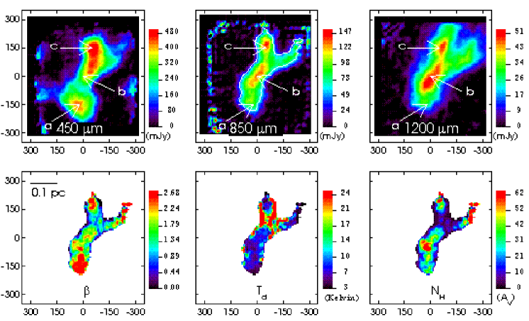
Figure 7: The 450, 850 and 1200 µm emission maps of TMC-1C, along with the derived $\beta$, $T_{d}$ and $N_{H}$ (expressed in units of $A_{V}$ for convenience). The fluxes are in units of mJy per 14″ pixel. The derived parameters are shown within the white 850 µm contour. The (0,0) position is at RA=4:41:35.8 DEC=+26:00:42.5 (J2000). Position ’a’ is strong at 450 µm but not at 850 or 1200 µm. Position ’b’ is strong at 850 and 1200 µm but not at 450 µm  and position ’c’ is strong in all three maps.

The original bowls of negative flux in our 450 µm map on either side of region ‘a’ in Figure 7 have peak values around $-150$ mJy, and average values around $-75$ mJy. We believe that these structures are artifacts of image reconstruction. It is possible that structures of similar magnitude (either positive or negative) might be affecting data elsewhere in the map.

2.2 MAMBO

We observed the 1.2 mm continuum emission in November 8, 2002, October 23, 2003, and November 2, 2003 using the 117-channel MAMBO-2 array (Kreysa et al., 1999) at the IRAM 30-meter telescope on Pico Veleta (Spain). The FWHM beam size on the sky was 10$\farcs$7. The source was mapped on-the-fly, with the telescope subreflector chopping in azimuth by 60″ to 70″ at a rate of 2 Hz; the total on-target observing time was about 6 hours. The line-of-sight optical depth varied between 0.1 and 0.5. The data were reconstructed using the EKH algorithm in an iterative way that properly reproduces large-scale emission (Kauffmann et al., in prep.). The rms noise in the 1200 µm map is 3 mJy/beam, measured in regions with no significant emission. The flux calibration uncertainty is approximately 10%, which is derived from the rms of calibrator observations across pool observing sessions and the uncertainty in the intrinsic calibrator fluxes.

3 Solving for physical parameters

In principal, one can use three measured quantities (e.g. the three flux density maps at 450, 850 and 1200 µm) to solve for three unknowns (e.g. maps of the dust temperature, emissivity spectral index, and column density). Our maps originally are in units of flux density per beam, with a different beam size for each map. To derive meaningful physical quantities we smooth and rebin our maps to a common resolution of the largest beam, which in our case is 14″. As a result, the quanity that we work with is flux density per 14″ pixel, which is what we present in our maps of TMC-1C.

The flux density per beam in each map is given by:

$$S_{\nu}=\Omega B_{\nu}(T_{d})\kappa_{{}_{\nu}}\mu m_{H}N_{H_{2}},$$ (1)

where

$$B_{\nu}(T_{d})=\frac{2h\nu^{3}}{c^{2}}\frac{1}{\exp(h\nu/kT_{d})-1}$$ (2)

and

$$\kappa_{{}_{\nu}}=\kappa_{230}\left(\frac{\nu}{230{\rm GHz}}\right)^{\beta}.$$ (3)

In Equation 1, $S_{\nu}$ is the flux density per 14″ pixel; $\Omega$ is the solid angle of the beam; $B_{\nu}(T_{d})$ is the blackbody emission from the dust at temperature $T_{d}$; $\kappa_{230}=0.009$ cm² g^-1 is the emissivity of the dust grains at 230 GHz (Ossenkopf & Henning, 1994); $m_{H}$ is the mass of the hydrogen atom; $\mu=2.8$ is the mean molecular weight of interstellar material in a molecular cloud per hydrogen molecule; $N_{H_{2}}$ is the column density of hydrogen molecules and a gas-to-dust ratio of 100 is assumed. It should be noted that $\kappa_{230}$ is uncertain by a factor of $\sim$2, and that we assumed that $\kappa_{230}=0.005$ and $\mu=2.33$ (which is the mean molecular weight per free particle for an abundance ratio of $N(H)/N(He)=10$ and negligible metals) in Schnee & Goodman (2005).

The ratio of two fluxes, because of the common beam size, can be simply expressed as:

$$\frac{S_{\nu_{1}}}{S_{\nu_{2}}}=\left(\frac{\nu_{1}}{\nu_{2}}\right)^{3+\beta}\left(\frac{\exp[h\nu_{2}/kT_{d}]-1}{\exp[h\nu_{1}/kT_{d}]-1}\right)$$ (4)

The dust temperature can be found independently of the dust emissivity spectral index by taking the difference between the ratio of fluxes, if we assume that each line of sight through the core can be characterized by a single temperature and emissivity spectral index:

$$\log\left(\frac{S_{450}}{S_{850}}\right)\log\left(\frac{1200\micron}{850\micron}\right)-$$

$$\log\left(\frac{S_{850}}{S_{1200}}\right)\log\left(\frac{850\micron}{450\micron}\right)=$$

$$\log\left(\frac{\exp\left[\lambda_{T}/850\micron\right]-1}{\exp\left[\lambda_{T}/450\micron\right]-1}\right)\log\left(\frac{1200\micron}{850\micron}\right)-$$

$$\log\left(\frac{\exp\left[\lambda_{T}/1200\micron\right]-1}{\exp\left[\lambda_{T}/850\micron\right]-1}\right)\log\left(\frac{850\micron}{450\micron}\right),$$ (5)

where $\lambda_{T}=hc/kT_{d}$.

Once the dust temperature is determined, the emissivity spectral index can be calculated by:

$$\beta=\log\left(\frac{S_{850}}{S_{1200}}\frac{\exp\left[\lambda_{T}/850\micron\right]-1}{\exp\left[\lambda_{T}/1200\micron\right]-1}\right)\left/\log\left(\frac{1200\micron}{850\micron}\right)\right.-3.$$ (6)

The column density of dust can be derived from the flux at a single wavelength (e.g. at 1200 µm), the temperature of the dust and the emissivity spectral index of the dust using Equation 1. The equivalent visual extinction can be calculated from the column density $N_{H}$ using:

$$A_{V}=N_{H}R_{V}\frac{E(B-V)}{N_{H}}$$ (7)

where $N_{H}=2\times N_{H_{2}}$, $N_{H}/E(B-V)=5.8\times 10^{21}$ cm^-2 mag^-1 is the conversion between column density of hydrogen nuclei (for our assumed gas to dust ratio) and the selective absorption, and $R_{V}=A_{V}/E(B-V)=3.1$ is the total to selective extinction ratio for the low-density lines of sight similar to those for which $N_{H}/E(B-V)$ has been measured (Mathis, 1990; Bohlin et al., 1978). Although we use a constant value of $R_{V}$, we recognize that this value is uncertain to within a factor of 2 between regions of high and low column density (Mathis, 1990), and the relation between extinction and column density may be different for dense cores like TMC-1C.

4 Error Analysis

In order to understand how the noise and reconstruction artifacts in our emission maps will affect the accuracy of our derived dust temperature, emissivity spectral index and column density we have run a variety of Monte Carlo simulations. We compare the effects of using maps at three particular wavelengths to solve for all three parameters to using the three measurements to fit for two parameters while assuming a fixed value for the third. We also show the improvements brought about by using a fourth wavelength and fitting for all three physical parameters.

4.1 Illustrative Examples

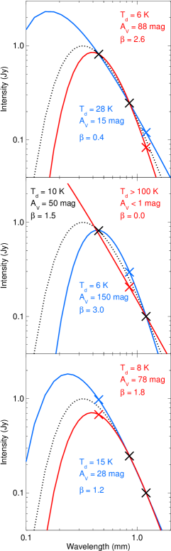
Figure 1: The true and calculated modified blackbody spectra of material with $A_{V}=50$, $\beta=1.5$ and $T_{d}=10$ K, observed with a 14″ beam. The black curve shows the true spectrum, and the black crosses show the flux at 450, 850 or 1200 µm. The blue and red crosses show the flux overestimated or underestimated, respectively, by 20%. The blue and red curves show the spectrum of dust that passes through the blue/red cross and the two black crosses. The dust temperature, emissivity spectral index and column density that would be derived from the three data points are also shown.

Here we discuss the uncertainties to be expected from solving for $T_{d}$, $\beta$ and $N_{H}$ from three emission maps that have noise or whose calibration is uncertain. To illustrate the method, Figure 1 shows the modified blackbody spectrum from dust with $A_{V}=50$, $T_{d}=10$ K and $\beta=1.5$, observed with a 14″ beam. The black dotted line shows the true emission spectrum, with crosses at 450, 850 or 1200 µm, and the blue/red crosses show the flux overestimated/underestimated at one wavelength by 20%. The blue and red curves are the fitted spectra that pass through the one blue/red cross and the two black crosses. It is clear that a 20% error in one measurement creates errors in all three derived parameters that are much larger than 20%. The derived values of $T_{d}$, $\beta$ and $N_{H}$ are labeled in Figure 1. For convenience, we show the derived $N_{H}$ in units of $A_{V}$.

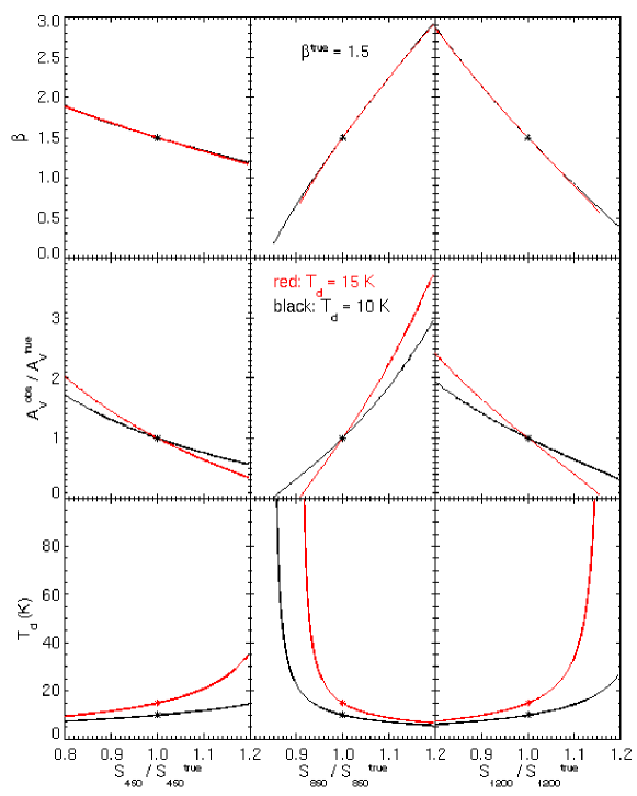
Figure 2: The derived emissivity spectral index ($\beta$), the ratio of the derived column density to the true column density and the derived temperature as functions of the ratio of the measured flux to the true flux at one wavelength (450, 850 or 1200 µm), with the other two fluxes measured without error. The black and red curves show the results for dust with $T_{d}=10$ K and $T_{d}=15$ K, respectively. $\beta=1.5$ in both cases. The curves are cut off where the derived temperature is greater than 100 K.

As can be seen from Equation 3, noise in any of the three flux maps first translates into uncertainty in the derived temperature. This incorrect value of $T_{d}$, along with any noise in the 850 and 1200 µm maps then results in uncertainties in the derived values of $\beta$ and $N_{H}$. From Equation 6, one can show that overestimating the temperature will result in an underestimate of $\beta$, and underestimating the temperature will result in an overestimate of $\beta$. The errors in the derived parameters from incorrectly measuring the flux at one wavelength, while correctly measuring the flux at the other two wavelengths is shown in Figure 2. The anti-correlation between $T_{d}$ and $\beta$ is clearly seen. Also apparent is that for dust with “core-like” values of $\beta$, $T_{d}$ and $N_{H}$, errors in 450 µm flux result in smaller errors in the derived physical parameters than errors at 850 and 1200 µm, which is convenient because the 450 µm maps often suffer from higher levels of noise than maps at 850 and 1200 µm.

4.2 Deriving the Physical Parameters

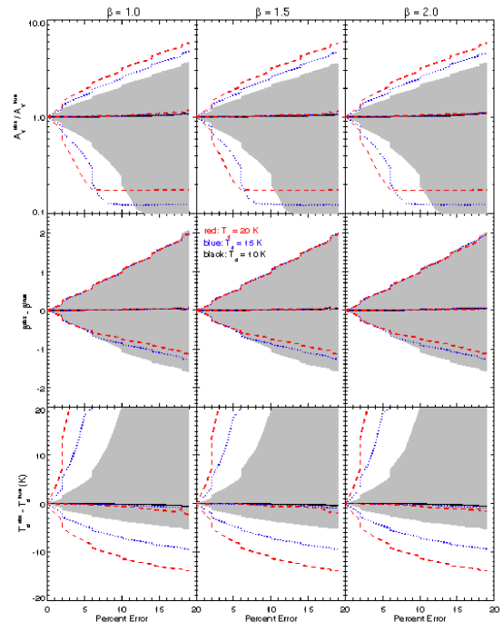
Figure 3: Each panel shows the 1$\sigma$ spread in the derived column density, temperature or emissivity spectral index as a function of the percent noise in all three flux maps at 450, 850 and 1200 µm. A 5% error in the measured flux corresponds to a signal to noise of 20. The black line shows the median value for the derived parameter, and the greyed area shows the 1 $\sigma$ spread in that parameter for dust at 10 K. The blue (dotted) and red (dashed) lines show the median value and 1 $\sigma$ spread for dust at 15 and 20 K, respectively, and each panel is repeated for emissivity spectral index ($\beta$ = 1.0, 1.5 or 2.0). $N_{H}$, $T_{d}$ and $\beta$ are derived as in Section 3. The column density is plotted as the ratio of the derived $A_{V}$ to the input $A_{V}$, and the temperature and emissivity spectral index are plotted as the difference between the derived parameter and the true value.

In order to determine the effect of similar levels of noise in all three wavelengths on the three derived physical parameters, we determine the flux at 450, 850 and 1200 µm from dust at $T_{d}=$ 10, 15 and 20 K and $\beta=$ 1.0, 1.5 and 2.0. The fluxes are then modified by a multiplicative factor $f=1.0+\delta$ where $\delta$ is randomly chosen from a normal distribution of mean zero and standard deviation $\sigma$, and each flux is modified by a different $f$. This is repeated 10,000 times for each value of $\sigma$ between 0 and 0.2. We show the effect of noise in all three wavelengths on the derived column density, temperature and emissivity spectral index in Figure 3. At a signal to noise of 20 (5% error), the expected uncertainties in the derived $N_{H}$, $T_{d}$ and $\beta$ are approximately 50%, 80% and 40%, respectively, for 15 K dust with $\beta=1.5$. The median values of the derived parameters stay close to the input values at every value of $T_{d}$ and $\beta$ tested.

The analysis presented here deals with the special case that the signal to noise is wavelength independent. In general, this will not be the case, and one might expect that for a given amount of observing time the signal to noise will be worse at 450 µm than at 850 or 1200 µm due to atmospheric effects. In addition, the relative signal to noise between maps will change from position to position, due to the gradients in the dust temperature, column density and emissivity spectral index. For instance, at the position of the column density peak in TMC-1C, the signal to noise ratios at 450, 850 and 1200 µm are 5.3, 27 and 33, respectively, when including both the random noise and the artifacts in the 450 µm image.

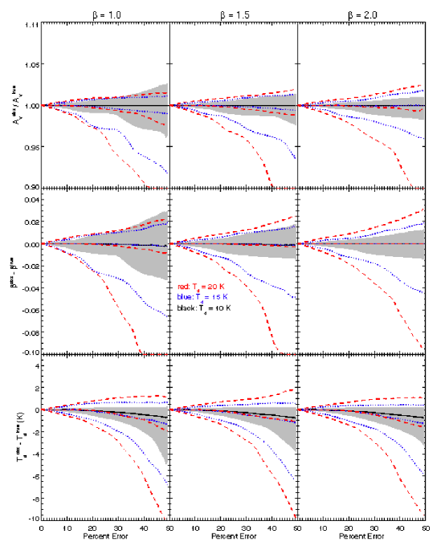
Figure 4: Same as Figure 3, except $N_{H}$, $T_{d}$ and $\beta$ are fit from four observations at 350, 450, 850 and 1200 µm.

Although even just 5% errors in the measured fluxes at three wavelengths make accurate determinations of three physical parameters impossible, adding a fourth wavelength (for instance, at 350 µm or 2.7 mm) drastically reduces the effects of noise, as can be seen by comparing Figure 3 with Figure 4. To properly constrain the dust parameters, at least one of the observations should not be on the Rayleigh-Jeans portion of the emission spectrum, or else $T_{d}$ and $N_{H}$ will be degenerate in the fit. For dust at $T_{d}=$ 10, 15 and 20 K and $\beta$ = 1.0, 1.5 and 2.0 we calculate the flux at 350, 450, 850 and 1200 µm. As before, the fluxes are then modified by a multiplicative factor $f=1.0+\delta$, where $\delta$ is again a variable randomly chosen from a normal distribution with mean zero and standard deviation $\sigma$. This is repeated 10,000 times for each value of $\sigma$ between 0 and 0.5. We allow $\sigma$ to be larger than in the previous Monte Carlo simulation because the effects of noise are smaller in this case. For each set of four fluxes, the column density, temperature and emissivity spectral index are fit and the results are shown in Figure 4. At a signal to noise of 20 (5% error), the expected errors in the column density, temperature and emissivity spectral index are all on the order of $\sim$1%. As the signal to noise gets lower, the median derived temperature and column density decrease, and this effect is larger for warmer cores.

4.3 Fixing One Parameter

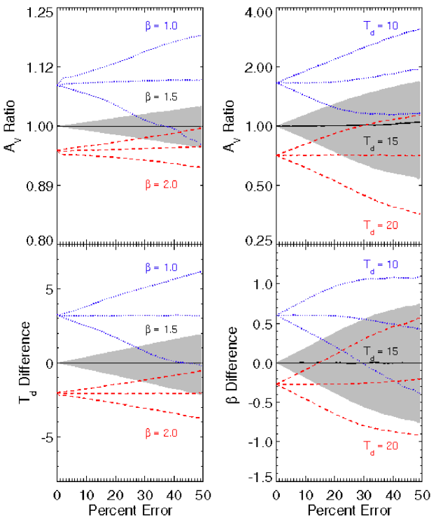
Figure 5: Each panel shows the 1 $\sigma$ spread in the derived $T_{d}$, $\beta$ and $N_{H}$ for dust at $T_{d}=15$ K and $\beta=1.5$ from a least squares fit between the predicted and given fluxes at 450, 850 and 1200 µm. The grey area uses the correct assumption that $\beta=1.5$ or $T_{d}=15$, while the blue (dotted) and red (dashed) lines incorrectly assume that $\beta=1.0$ and $\beta=2.0$, or $T_{d}=10$ and $T_{d}=20$, respectively.

In the case of a starless core observed at three wavelengths, one can hold one parameter fixed, such as assuming a constant $T_{d}=15$ K or $\beta=1.5$, and use the three flux measurements to fit the remaining two parameters. Figure 5 shows the result of using noisy flux measurements to fit the column density and either the dust temperature or the emissivity spectral index of a core with $T_{d}=$ 15 K and $\beta=$ 1.5. We show the results for correctly assuming that $\beta=1.5$ and erroneously assuming that $\beta=$ 2.0 or 1.0, as well as for correctly assuming that $T_{d}=$ 15 K and erroneously assuming that $T_{d}=$ 10 or 20 K.

We see that by choosing the correct value of $\beta$ and fitting the $T_{d}$ and $N_{H}$, noise in the emission maps on the level of 10% result in $\sim$1% uncertainties in the derived temperature and column density. Choosing a value of $\beta=1.0$, when the proper value is $\beta=1.5$ results in temperatures that are on average 3 K too high, with a spread of $\sim$3 K, and column densities that are high by 8%. Overestimating the emissivity spectral index, by assuming that $\beta=2.0$, results in temperatures that are on average 2 K too low and column densities that are 5% low.

Figure 5 shows that by choosing the $T_{d}$ and fitting for the $\beta$ and $N_{H}$, the true values of $\beta$ and column density are recovered, on average, with an absolute spread of 0.20 in $\beta$ and a relative spread of 13% in column when the signal to noise ratio is 10. Underestimating the temperature by assuming $T_{d}=10$ K when the proper value is $T_{d}=15$ K results in an overestimate of the emissivity spectral index by 0.6, on average, and an overestimate of the column density by 70%. Overestimating the temperature by assuming that $T_{d}=20$ K results in an underestimate of $\beta$ by 0.3, on average, and an underestimate of $N_{H}$ by a factor of 30%.

4.4 A Model Core

We apply the error analysis presented in Section 4 to our data on the starless core TMC-1C in order to derive new science beyond what was possible in our earlier paper on this core (Schnee & Goodman, 2005). The random noise in the emission maps, as measured in regions with faint emission, is found to be 13 mJy/beam, 9 mJy/beam and 3 mJy/beam, which corresponds to S/N values of 21, 14 and 15 at 450, 850 and 1200 µm at the (0,0) position of the emission maps. Calibration uncertainties are $\sim$12%, 4% and 10% at 450, 850 and 1200 µm, respectively, and the image reconstruction artifacts in the 450 µm map peak at 150 mJy/beam.

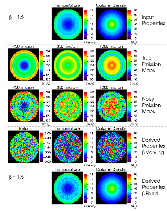
Figure 6: The top row of panels shows the temperature and column density maps of a model starless core similar to the central 2′ of TMC-1C. The second row shows the predicted emission maps at 450, 850, and 1200 µm, using a constant $\beta=1.5$. We then add Gaussian random noise to the emission maps equal to the measured noise and artifacts in our 450, 850 and 1200 µm maps of TMC-1C (80, 9 and 3 mJy, respectively) and show the resultant fluxes in the third row. Using the altered fluxes, we attempt to solve for $\beta$, $T_{d}$ and $N_{H}$ at each point in the map, and show the results in the fourth row from the top. When we use the value $\beta=1.5$ everywhere along with the altered 450, 850 and 1200 µm fluxes to fit $T_{d}$ and $N_{H}$, we derive the maps shown in the bottom row.

To determine how the random noise and reconstruction artifacts (which are spatially correlated and therefore not truly random) in the observed emission maps affect the derived parameters, we construct synthetic emission maps of a starless core like TMC-1C. The model core has a temperature and column density profile equal to the one derived from the two dimensional temperature and column density profile of TMC-1C, derived from fitting the 450, 850 and 1200 µm data and assuming a constant $\beta=1.5$. The model starless core is made of cylindrical shells seen face on with a central temperature of $\sim$6 K, rising to $\sim$12 K at the edge. The central column density corresponds to $\sim$80 magnitudes of visual extinction, falling to an $A_{V}$ of $\sim$20 at the edge. Using the equations in Section 3, we derive the resultant emission maps at 450, 850 and 1200 µm, add in Gaussian noise of the same magnitude as the random noise and reconstruction artifacts described above, and from these emission maps derive maps of the column density, temperature and emissivity spectral index. The resultant maps are shown in Figure 6.

The dust emission in our model core (shown in Figure 6) at 450 and 850 µm is not a good tracer the dust column density, though the 1200 µm emission map does resemble the column density distribution. Spatial gradients in the dust properties, such as the temperature and emissivity spectral index, need to be taken into account when attempting to find the “peak” of the dust distribution, even when using the relatively longer wavelength 1200 µm emission map as a proxy for column density.

When we solve for all three physical parameters, we find that the derived $\beta$ of our model cloud has a median value of 1.5 (which is the input $\beta$ everywhere in the model) with a standard deviation of 0.7. Given the close correspondence between the input value of $\beta$ and the median value derived for it, we see that a constant value for the emissivity spectral index can be estimated in this manner. Using this constant value for $\beta$ everywhere, we can then use our three flux maps to fit the temperature and column density. The resultant maps of our model constructed in this way are shown in Figure 6. Although using the median value in the $\beta$ map to derive a constant value for the emissivity spectral index reduces the impact of statistical uncertainty due to random noise, systematic shifts, such as those created from calibration uncertainties, are not removed.

5 Dust Emission in TMC-1C

5.1 Morphology

The observed 450 µm emission map of TMC-1C is qualitatively different from the 1200 µm map. The 450 µm map shows a condensation at $(50,-150)$ (position “a” in Figure 7) which is much fainter at 850 µm and nearly absent at 1200 µm. The condensation at $(-50,150)$ (position “c” in Figure 7) is prominent at all wavelengths, while the column density peak at $(0,0)$ (position “b” in Figure 7) is prominent at 850 and 1200 µm, but not apparent at 450 µm.

An emission peak in the longer wavelength maps, but not prominent at 450 µm, can be explained by a cold temperature, as seen at the $(0,0)$ position. The 450 µm emission peak not seen at 1200 µm can be explained by the dust in that region having a steep spectral index ($\beta\geq 2$).

5.2 Derived Parameters

Based on our analysis in Section 4.1, calibration uncertainties, reconstruction artifacts and noise in our TMC-1C emission maps prevent us from making accurate maps of dust temperature, emissivity spectral index and column density simultaneously, even though this may well be the highest S/N set of such maps of a starless core to date. Figure 7 shows the results of an attempt to do so, and as expected the range of temperatures that we see is quite broad ($T_{d}<5$ K and $T_{d}>25$ K) for a starless core, with a similarly large spread in emissivity spectral index ($\beta<0$ and $\beta>2.5$) and column density. Furthermore, the errors and uncertainties in our emission maps create a spurious anti-correlation between the dust temperature and emissivity spectral index, which is also seen in our attempt to derive $T_{d}$, $\beta$ and $N_{H}$ from our simple model of a cylindrically symmetric starless core, described in Section 4.4. Because the noise and errors in our observed emission maps of TMC-1C will drive an anti-correlation between the derived dust temperature and emissivity spectral index even when such a trend does not exist, our results are consistent with a constant value of the emissivity spectral index. However, we cannot rule out a real anti-correlation such as that observed at 200, 260, 360 and 580 µm in the Orion molecular cloud (Dupac et al., 2001) and the M17 star-forming complex (Dupac et al., 2002).

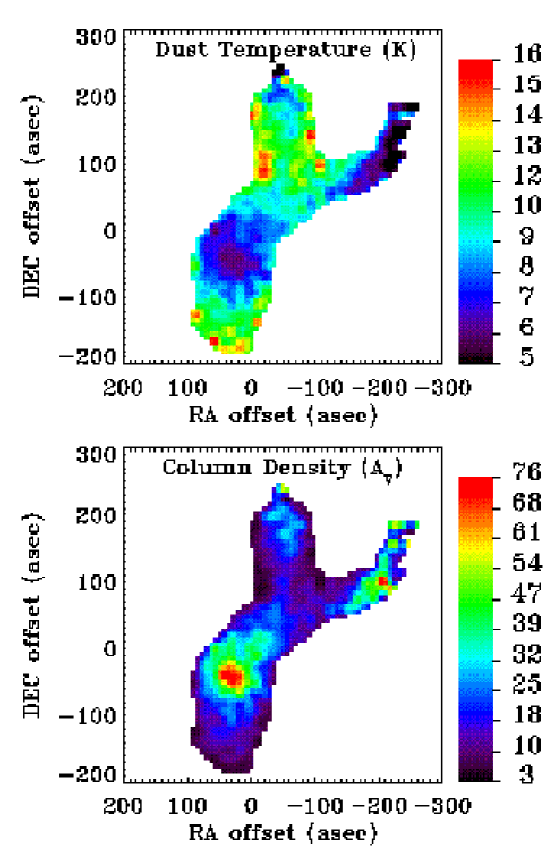
Figure 8: The TMC-1C dust color temperature (top) and column density (bottom), derived from a fit to the 450, 850 and 1200 µm emission maps, assuming that the emissivity spectral index is constant at $\beta=1.8$.

Following the method described in Section 4.4, we take the median value of the emissivity spectral index map (Figure 7) and derive a value and uncertainty of $\beta=1.8\pm 0.5$ for the portion of TMC-1C located within the white contour of the 850 µm image in Figure 7. Unless otherwise state, in our subsequent analysis of TMC-1C we use a constant value of $\beta=1.8$ everywhere in the core. We derive $\beta$ and the 1$\sigma$ uncertainty by running 1000 realizations of a Monte Carlo simulation of the observed flux maps in TMC-1C modified by the calibration uncertainties. Using $\beta=1.8$, we construct dust temperature and column density maps (Figure 8) from a fit to the 450, 850 and 1200 µm images. The column density in Figure 8 peaks around the maximum of the 850 and 1200 µm emission. The implied visual extinction is quite high, rising above 80 magnitudes in the densest regions. As expected, the regions with the highest column density are also the regions with the lowest dust temperature (Zucconi et al., 2001). By using a constant value of the emissivity spectral index ($\beta=1.8$), the dust temperature that we derive is nowhere significantly higher than 16 K nor lower than 6 K.

Our derived value of $\beta=1.8\pm 0.5$ is somewhat higher than that measured for amorphous carbon grains ($\beta=1.2$) by Mennella et al. (1998) and is within the range ($\sim 1.2-2.5$) measured for silicate grains by Agladze et al. (1996). Dust in interstellar disks are generally observed to have values of $\beta\leq 1$, but with considerable spread (Beckwith & Sargent, 1991; Mannings & Emerson, 1994). Observations by Stepnik et al. (2003) have shown that $\beta=1.9\pm 0.2$ for a dense filament in Taurus, which agrees very well with our estimate of TMC-1C. Graphite and silicate dust grains in the ISM are often assumed to have $\beta=2$ (e.g. Draine & Lee, 1984).

5.3 Comparison With Previous Results

Two-dimensional temperature and column density maps of TMC-1C, along with the deprojected three-dimensional temperature and density profiles, have previously been reported in Schnee & Goodman (2005) using only SCUBA 450 and 850 µm data. With the addition of the MAMBO 1200 µm map, we are better able to constrain the temperature and density and estimate the emissivity spectral index. The emissivity spectral index that we use here ($\beta=1.8$) is higher than in Schnee & Goodman (2005) ($\beta=1.5$), because in this paper we are able to derive $\beta$, and in our ealier work we had to assume a value. The value that we use in this paper for $\kappa_{230}$ is taken from Ossenkopf & Henning (1994), which is larger than the number we used in Schnee & Goodman (2005). As a result using larger $\beta$ and $\kappa_{230}$, the temperatures that we derive are somewhat lower and the densities are also lower. We choose here to use the dust opacity appropriate for dust grains with thin ice mantles, evolved in a dense (10⁶ cm^-3) region for 10⁵ years derived in Ossenkopf & Henning (1994) because this is the consensus value settled upon by the Spitzer Legacy Project, “From Molecular Cloud Cores to Planet Forming Disks” (Evans et al., 2003), which will make comparisons with other c2d cores easier in the future. The mass that we derive for TMC-1C, within a radius of 0.06 pc from the column density peak is 6 M_⊙, as compared with 13 M_⊙ in Schnee & Goodman (2005). However, even this new dust-derived mass is higher than the virial mass derived from TMC-1C N₂H⁺ observations.

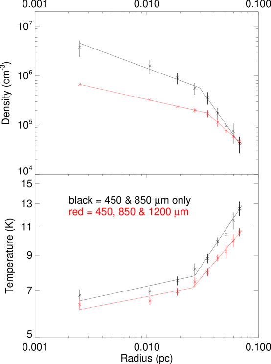
Figure 9: The density (top) and temperature (bottom) profiles of TMC-1C. The points in red are determined by a fit to the 450, 850 and 1200 µm data, assuming $\beta=1.8$ and $\kappa_{230}=0.009$ and the black points are determined using only the 450 and 850 µm data assuming $\beta=1.5$, as in Schnee & Goodman (2005) and $\kappa_{230}=0.005$, as assumed here. In both cases, we assume that the central 2 arcminute radius of TMC-1C can be modeled as nested spherical shells of uniform density and temperature.

Following the method used in Schnee & Goodman (2005), we create deprojected three dimensional temperature and density profiles. We assume that the inner 0.07 pc of TMC-1C can be approximated as a set of nested spherical shells, each with a constant temperature and density. The derived temperature and density profiles are shown in Figure 9, along with the profiles calculated using only the 450 and 850 µm data and assuming that $\beta=1.5$, as in Schnee & Goodman (2005). The dust temperature profile that we derive is not much changed from that derived in Schnee & Goodman (2005), and is thus still consistent with the dust temperature profiles predicted for externally heated starless cores with Bonnor-Ebert density distributions calculated by Evans et al. (2001); Gonçalves et al. (2004); Stamatellos et al. (2004). A Bonnor-Ebert profile is a good fit to the TMC-1C density profile at radii greater than 0.004 pc, but as in Schnee & Goodman (2005), the density we derive for the innermost point is significantly higher than predicted by a Bonnor-Ebert model. The density profile, shown in Figure 9, is consistent with a broken powerlaw, with $n(r)\propto r^{-0.5}$ inside 0.035 pc and $n(r)\propto r^{-2.0}$ outside 0.035 pc. This is considerably flatter than the density profile derived using only the 450 and 850 µm data and $\beta=1.5$, which have powerlaw exponents of $-0.8$ and $-3.1$ inside and outside the break radius, respectively (also shown in Figure 9). In Schnee & Goodman (2005) we report inner and outer powerlaw exponents of $-0.8$ and $-1.8$, also using just the 450 and 850 µm data and $\beta=1.5$, but using a slightly different position as the center of the nested spherical shells, so the comparison of powerlaw exponents presented in Schnee & Goodman (2005) and those present here would be unfair. Also note that the central density of TMC-1C that we derive from the 450, 850 and 1200 µm maps is a factor of $\sim$5 lower than when derived using just the 450 and 850 µm maps (and assuming $\beta=1.5$), which shows the significant adjustments that can result from utilizing additional emission maps. An improved value of the central density can make a significant impact on the predictions of the dynamical state of a core, and on chemical models.

6 Summary

We have used SCUBA data at 450 and 850 µm and MAMBO data at 1200 µm to create maps of the dust temperature and column density in TMC-1C, improving the results presented in Schnee & Goodman (2005). In addition, we are able to estimate the emissivity spectral index, finding a value of $\beta=1.8\pm 0.5$, based on calibration uncertainties.

Our analysis shows that noise and calibration errors in maps at 450, 850 and 1200 µm would have to be less than $\sim$2% to accurately measure the dust temperature, emissivity spectral index and column density from three emission maps. Although such low levels of noise and calibration uncertainties are not achievable with the current generation of bolometers, we show that the dust temperature, emissivity spectral index and column density can be accurately mapped if they are fitted at four wavelengths, for instance by including the 350 µm SHARCII waveband. Obtaining accurate maps of $T_{d}$, $\beta$ and $N_{H}$ are necessary for accurate determinations of density and temperature profiles as well as the core mass, which determine the time evolution and chemistry of the core.

The next generation detectors on the JCMT (SCUBA-2) and on APEX (LABOCA), will not need to sky-chop, allowing more large-scale structure to be visible, improved calibration and fewer image artifacts, making more accurate determinations of dust properties in cores possible (Ellis, 2005; Güsten et al., 2006).

References

- Agladze et al. (1996) Agladze, N. I., Sievers, A. J., Jones, S. A., Burlitch, J. M., & Beckwith, S. V. W. 1996, ApJ, 462, 1026
- Barranco & Goodman (1998) Barranco, J. A., & Goodman, A. A. 1998, ApJ, 504, 207
- Beckwith & Sargent (1991) Beckwith, S. V. W., & Sargent, A. I. 1991, ApJ, 381, 250
- Bianchi et al. (2000) Bianchi, S., Davies, J. I., Alton, P. B., Gerin, M., & Casoli, F. 2000, A&A, 353, L13
- Bohlin et al. (1978) Bohlin, R. C., Savage, B. D., & Drake, J. F. 1978, ApJ, 224, 132
- Draine & Lee (1984) Draine, B. T., & Lee, H. M. 1984, ApJ, 285, 89
- Dupac et al. (2002) Dupac, X., et al. 2002, A&A, 392, 691
- Dupac et al. (2001) Dupac, X., et al. 2001, ApJ, 553, 604
- Ellis (2005) Ellis, M. 2005, Experimental Astronomy, 19, 169
- Evans et al. (2003) Evans, N. J., II, et al. 2003, PASP, 115, 965
- Evans et al. (2001) Evans, N. J., II, Rawlings, J. M. C., Shirley, Y. L., & Mundy, L. G. 2001, ApJ, 557, 193
- Gonçalves et al. (2004) Gonçalves, J., Galli, D., & Walmsley, M. 2004, A&A, 415, 617
- Goodman et al. (1998) Goodman, A. A., Barranco, J. A., Wilner, D. J., & Heyer, M. H. 1998, ApJ, 504, 223
- Goodman et al. (1993) Goodman, A. A., Benson, P. J., Fuller, G. A., & Myers, P. C. 1993, ApJ, 406, 528
- Güsten et al. (2006) Güsten, R., Nyman, L. Å., Schilke, P., Menten, K., Cesarsky, C., & Booth, R. 2006, A&A, 454, L13
- Holland et al. (1999) Holland, W. S., et al. 1999, MNRAS, 303, 659
- Johnstone et al. (2000) Johnstone, D., Wilson, C. D., Moriarty-Schieven, G., Joncas, G., Smith, G., Gregersen, E., & Fich, M. 2000, ApJ, 545, 327
- Kenyon et al. (1994) Kenyon, S. J., Dobrzycka, D., & Hartmann, L. 1994, AJ, 108, 1872
- Kreysa et al. (1999) Kreysa, E., Gemünd, H.-P., Gromke, J. 1999 Infrared Phys. Techn. 40, 191
- Mannings & Emerson (1994) Mannings, V., & Emerson, J. P. 1994, MNRAS, 267, 361
- Mathieu et al. (1995) Mathieu, R. D., Adams, F. C., Fuller, G. A., Jensen, E. L. N., Koerner, D. W., & Sargent, A. I. 1995, AJ, 109, 2655
- Mathis (1990) Mathis, J. S. 1990, ARA&A, 28, 37
- Mennella et al. (1998) Mennella, V., Brucato, J. R., Colangeli, L., Palumbo, P., Rotundi, A., & Bussoletti, E. 1998, ApJ, 496, 1058
- Ossenkopf & Henning (1994) Ossenkopf, V., & Henning, T. 1994, A&A, 291, 943
- Pierce-Price et al. (2000) Pierce-Price, D., et al. 2000, ApJ, 545, L121
- Reid & Wilson (2005) Reid, M. A., & Wilson, C. D. 2005, ApJ, 625, 891
- Schnee & Goodman (2005) Schnee, S., & Goodman, A. 2005, ApJ, 624, 254
- Stamatellos et al. (2004) Stamatellos, D., Whitworth, A. P., André, P., & Ward-Thompson, D. 2004, A&A, 420, 1009
- Stepnik et al. (2003) Stepnik, B., et al. 2003, A&A, 398, 551
- Zucconi et al. (2001) Zucconi, A., Walmsley, C. M., & Galli, D. 2001, A&A, 376, 650