Metal mixing by buoyant bubbles in galaxy clusters

Abstract

Using a series of three-dimensional, hydrodynamic simulations on an adaptive grid, we have performed a systematic study on the effect of bubble-induced motions on metallicity profiles in clusters of galaxies. In particular, we have studied the dependence on the bubble size and position, the recurrence times of the bubbles, the way these bubbles are inflated and the underlying cluster profile. We find that in hydrostatic cluster models, the resulting metal distribution is very elongated along the direction of the bubbles. Anisotropies in the cluster or ambient motions are needed if the metal distribution is to be spherical. In order to parametrise the metal transport by bubbles, we compute effective diffusion coefficients. The diffusion coefficients inferred from our simple experiments lie at values of around $\sim 10^{29}$ cm²s^-1 at a radius of 10 kpc. The runs modelled on the Perseus cluster yield diffusion coefficients that agree very well with those inferred from observations.

1 Introduction

The hot, diffuse gas that permeates clusters of galaxies, the intra-cluster medium (ICM), has a metallicity of about 1/3 of the solar value. Meanwhile, the total amount of iron in the ICM is huge: it is larger than the total iron mass in all cluster galaxies. Moreover, this value does not seem to vary much with time, at least not up to a redshift of $\sim 1$ (Tozzi et al. 2003). The recent generation of X-ray observatories has provided maps of the radial distribution of metals in the nearby clusters (De Grandi & Molendi 2001; Fukazawa et al. 2000; Schmidt et al. 2002; Matsushita et al. 2002; Churazov et al. 2003; De Grandi et al. 2004; Tamura et al. 2004). These observations have revealed an interesting trend:

Galaxy clusters can be grouped into two categories depending on their X-ray surface brightness profiles: (i) clusters with a central peak in the X-ray surface brightness, i.e. clusters with a cool core and (ii) clusters without a cool core. Interestingly, these two groups show a different spatial distribution of metals. The clusters without cool cores have a nearly uniform spatial distribution of metals, while clusters with cool cores have a strongly peaked abundance profile. Moreover, the relative abundance of elements in cool core clusters suggests that Type Ia supernovae have provided most of the metals in the central iron peak. Finoguenov et al. (2002) have found that the central abundance peak is strongly enriched in iron while the bulk of the ICM outside the central region had an iron-to-silicon ratio close to the yields of Type II supernovae (also Mushotzky et al. 1996). This suggests that the central metal peak is mostly caused by Type Ia supernovae in the central cluster galaxy. However, in order to produce the large mass of metals in the central peak, long enrichment times are necessary.

There are a number of observations that indicate that stars in massive galaxies are responsible for the metal enrichment of the ICM. It has been established that the iron mass of the ICM correlates with the optical light of massive early-type galaxies in clusters (Arnaud et al. 1992) and that the ratio of the iron mass to light and to the total mass is approximately constant. Thus, stellar mass loss from the central cluster galaxy through supernovae and stellar winds appears to be the prime source for the metals observed in the inner parts of galaxy clusters. However, the observed metallicity profiles are much broader than the stellar light profiles of the central galaxy. Hence, the differences in the light and metal distributions are interpreted as the result of transport processes that have mixed the metals into the ICM. Rebusco et al. (2005) have assumed that the spreading is due to local turbulent motions in the ICM, and that the evolution of the metal density profile can be modelled as a diffusion process. Using the abundance profile from Churazov et al. (2003) for Perseus, Rebusco et al. (2005) estimated that a diffusion coefficient of the order of $2\times 10^{29}~{}{\rm cm^{2}~{}s^{-1}}$ is needed to explain the width of the observed abundance profiles. Based on a model of iron enrichment from stellar mass loss in the central cluster galaxies of a few nearby clusters, Böhringer et al. (2004) have used the total amount of iron observed in the ICM to obtain constraints on the age of the cooling cores (i.e. the time for which the central region have remained relatively undisturbed). They find very large ages of more than 7 Gyr (Böhringer et al. 2004) that provide new constraints for the modelling of the interaction regions and have consequences for the turbulent transport of metals. While it appears to be established that the metals produced by the central galaxy are dispersed into the ICM to form the broad abundance peaks, it remains unclear what the mechanism is via which the metals are transported.

Currently, the most popular model that is invoked to explain the apparent stability of cool cores against a cooling catastrophe relies on heating by a central Active Galactic Nucleus (AGN). Radio-loud AGN are also thought to regulate the formation of the most massive galaxies and thus explain the cut-off of the galaxy luminosity function at the bright end (Croton et al. 2006). Radio-loud active galactic nuclei drive strong outflows in the form of jets that inflate bubbles or lobes. The lobes are filled with hot plasma, and can heat the cluster gas in a number of ways (e.g. Brüggen et al. 2002; Brüggen & Kaiser 2002; Churazov et al. 2001; Dalla Vecchia et al. 2004; Omma et al. 2004; Basson & Alexander 2003; Reynolds et al. 2002; Ruszkowski et al. 2004; Brüggen et al. 2005; Brighenti & Mathews 2006).

In fact, radio sources in cooling clusters are different from the general population of radio sources in galaxy clusters. Most radio galaxies in clusters are FR I sources in terms of their radio power, but they show a great variety of morphologies and dynamics (Owen & Ledlow 1997). The central galaxy in almost every strong cooling core contains an active nucleus and a currently active, jet–driven radio galaxy. High-resolution X-ray observations of cooling flow clusters with Chandra have revealed a multitude of X-ray holes on scales $<$ 50 kpc, often coincident with patches of radio emission. In a recent compilation, Bîrzan et al. (2004) lists 18 well documented clusters which show X-ray cavities with radio emission.

Buoyantly rising bubbles induce subsonic motions in the cluster gas that can redistribute metals in the ICM (Brüggen 2002). Considering the impact of resonant scatterings on the surface brightness profile of the most prominent X-ray emission lines, evidence for gas motions was found in the XMM-Newton data on the Perseus cluster (Churazov et al. 2004). The same motions could spread the metals over the cluster volume although the efficiency of spreading could be very sensitive to the character of these motions. Other enrichment mechanisms include supernovae-driven winds, radiation-pressure-driven dust efflux (see e.g. Aguirre et al. 2001) and ram pressure stripping of cluster galaxies (Roediger & Brueggen 2005; Roediger et al. 2006). Using cosmological simulations and a heuristic prescription for the effect of ram-pressure stripping, Domainko et al. (2006) find that ram-pressure stripping can account for $\sim$10% of the overall observed level of enrichment in the ICM within a radius of 1.3 Mpc (see also Tornatore et al. 2004). Furthermore, Schindler et al. (2005) find that ram-pressure stripping is more efficient than quiet (i.e. non-starburst driven) galactic winds, at least in recent epochs since redshift 1. Also, they find that the expelled metals are not mixed immediately with the ICM, but inhomogeneities are visible in the metallicity maps. Relatively little theoretical work has gone in establishing the importance of AGN-induced transport of metals in cluster centres (Brüggen 2002, Omma et al. 2004). However, this mode is likely to be very important, at least at redshifts $\leq 1$: If AGN-induced motions are sufficient to quench cooling flows at the centres of galaxy clusters, they are similarly likely to affect the metal distribution in the central cluster region. Simulations as those presented here are essential for a proper modelling of the chemical evolution of clusters via semi-analytical techniques, as for example in De Lucia et al. (2004); Cora (2006).

The broad abundance peaks in clusters have been produced over a time span of several gigayears. If the peaks have been broadened by AGN, this process has taken a large number of activity cycles. In order to simulate the transport of metals by AGN-induced flows and to capture the hydrodynamical details important for the interaction between the AGN and the ICM, a fair resolution of the computational mesh is necessary. This prevents us from simulating the bubble transport over cosmological times. However, we can still study the efficiency of the metal transport by simulating a small number of AGN cycles and parametrise the transport efficiency. A convenient parametrisation that has been applied previously to observations (Rebusco et al. 2005) is based on a diffusion description. Even though we do not propose that the metal transport occurs via microscopic diffusion, transport processes like these may be described by a diffusion parameter. This allows a direct comparison to observations without having to simulate the entire life time of the cluster.

In this paper, we investigate the influence of buoyantly rising bubbles in clusters on the metal distribution in the ICM. In particular, we focus on the following questions:

• How far out can bubbles carry metals?

• How efficient is transport by buoyant bubbles?

• Does this process cause characteristic features, e.g. anisotropies?

• How does the resulting metal distribution depend on bubble and cluster parameters?

• What effective diffusion coefficients does this form of transport yield?

• How do these coefficients compare with those found by Rebusco et al. (2005)?

To this end, we simulated the effect of bubble-induced motions in the ICM based on the 3D hydrodynamics code FLASH.

2 Method

2.1 Overview

We model the hydrodynamical evolution of the ICM in a galaxy cluster. Initially, the ICM is set in hydrostatic equilibrium in a static cluster potential. Details of the ICM model are given in Sect. 2.3.1.

We assume that a central cluster galaxy injects metals into the ICM with a rate proportional to its light distribution. Details of the central galaxy are given in Sect. 2.3.2. We now trace the distribution of the metals by injecting a tracer fluid into the ICM at a rate that is proportional to the light distribution of the central galaxy. Section 2.4 explains the details of the metal injection and the way the metals are traced throughout the simulation.

Finally, we model the AGN activity by inflating ambipolar pairs of underdense bubbles in the ICM that rise buoyantly and thus stir the ICM. In Section 2.5 we explain in detail how the bubbles are generated.

2.2 Code

The simulations were performed with the FLASH code (Fryxell et al. 2000), a multidimensional adaptive mesh refinement code. FLASH is a modular block-structured AMR code, parallelised using the Message Passing Interface (MPI) library. It solves the Riemann problem on a Cartesian grid using the Piecewise-Parabolic Method (PPM). The simulations are performed in 3D and all boundaries are reflecting. We use a simulation box of size $(x_{\mathrm{min}},x_{\mathrm{max}})\times(y_{\mathrm{min}},y_{\mathrm{max}})\times(z_{\mathrm{min}},z_{\mathrm{max}})=(-145\,\textrm{kpc},145\,\textrm{kpc})^{3}$. The cluster centre is located at $(x_{\mathrm{cluster}},y_{\mathrm{cluster}},z_{\mathrm{cluster}})=(0,0,0)$. For our grid, we chose a block size of $16^{3}$ zones. The unrefined root grid contains $6^{3}$ blocks. The refinement criteria are the standard density and pressure criteria. In the central $\sim 30\,\textrm{kpc}$, the grid is assigned a minimum refinement level of 3. Outside $\sim 100\,\textrm{kpc}$, the refinement is restricted to a maximum of 5 levels to limit the computational effort. The resulting resolutions for the different runs are summarised in Table 3.

There have been some suggestions that the ICM may have a non-negligible viscosity (Reynolds et al. 2005; Ruszkowski et al. 2004). However, the effective viscosity of the ICM remains unknown because the physics of such dilute and magnetised plasmas is poorly constrained. In particular, the effect of magnetic fields on the macroscopic viscosity is unclear. Even minute magnetic fields lead to small proton gyroradii and are thus expected to suppress the viscosity efficiently. However, it has been pointed out that the exponential divergence of neigbouring field lines in a tangled magnetic field may lead to only a very modest suppression of the viscosity. Reynolds et al. (2005) have simulated the buoyant rise of bubbles in a medium with a kinematic viscosity. They found that even a modest shear viscosity (corresponding to 1/4 of the Spitzer value) can quench fluid instabilities and keep the bubbles intact (especially see figure 4 in their paper). Other simulations of buoyant bubbles in a viscous ICM were performed by Sijacki & Springel (2006) using smoothed particle hydrodynamics.

FLASH solves the equations of inviscid hydrodynamics. The Piecewise-Parabolic Method uses a monotonicity constraint rather than artificial viscosity to control oscillations near discontinuities. However, the discretisation of the equations still leads to a numerical viscosity. A comparison with the simulations of bubbles in a viscous medium by Reynolds et al. (2005) (cf. with their figure 4) shows that the Reynolds number in our simulations is $>1000$.

Except by the effect of viscosity, bubbles can be stabilised by magnetic fields. It has been known for some time that the hot gas in clusters of galaxies hosts significant magnetic fields (Carilli & Taylor, 2002), with estimated typical magnetic field strengths of $5\times 10^{-6}$ G (5 $\mu$G). A magnetic field tangential to the fluid interface can stabilise the Rayleigh-Taylor instability (Chandrasekhar, 1961), provided the restoring tension generated by bending of the field lines exceeds the buoyancy force driving the instability. The stabilising effect of intracluster magnetic fields was pointed out by De Young (2003), who derived analytic conditions for the stabilisation of relic radio bubbles in the hot ICM. These calculations showed that the field strengths observed in many clusters will stabilise the bubble interface in the linear regime, and hence the cluster magnetic fields could account for why the relic radio bubbles are seen as intact objects at such late times. Additional support for this idea is found in the two-dimensional MHD calculations of Brüggen & Kaiser (2001), who applied a $\beta\sim 10$ field inside the bubbles that was aligned with the bubble surface. While viscosity and magnetic fields can affect the dynamics of the bubbles and thus also the resultant transport of metals, the effects are still poorly understood. Here we only study the case of inviscid and unmagnetised fluids.

2.3 Model cluster

2.3.1 ICM distribution

In this paper, we study two different cluster models. In the first, generic one, we take a constant ICM temperature and the pressure is set by assuming hydrostatic equilibrium. Table 1 lists the ICM parameters.

The density of the ICM follows a $\beta$-profile,

$$\rho_{\mathrm{ICM}}(r)=\rho_{\mathrm{ICM}}{}_{0}\left[1+\left(\frac{r}{R_{\mathrm{ICM}}}\right)^{2}\right]^{-3/2\beta}$$ (1)

Table 1: ICM parameters for generic runs.

$R_{\mathrm{ICM}}$	$50\,\textrm{kpc}$
$\rho_{\mathrm{ICM}}{}_{0}$	$10^{-26}\,\textrm{g}\,\textrm{cm}^{-3}$
$\beta$	$0.5$
$T_{\mathrm{ICM}}$	$4.7\cdot 10^{7}\,\textrm{K}$

In addition to the generic cluster model, we set up a cluster modelled on the brightest X-ray cluster A426 (Perseus) that has been studied extensively with Chandra and XMM-Newton.

The electron density $n_{\rm e}$ and the temperature $T_{\rm e}$ profiles used here are based on the deprojected XMM-Newton data (Churazov et al. 2003, 2004) which are also in broad agreement with the ASCA (Allen & Fabian 1998), Beppo-Sax (De Grandi & Molendi 2001, 2002) and Chandra (Schmidt et al. 2002, Sanders et al. 2004) data. Namely:

$$n_{\rm e}=\frac{4.6\times 10^{-2}}{[1+(\frac{r}{57})^{2}]^{1.8}}+\frac{4.8\times 10^{-3}}{[1+(\frac{r}{200})^{2}]^{0.87}}~{}~{}~{}{\rm cm}^{-3}$$ (2)

and

$$T_{\rm e}=7\times\frac{[1+(\frac{r}{71})^{3}]}{[2.3+(\frac{r}{71})^{3}]}~{}~{}~{}{\rm keV},$$ (3)

where $r$ is measured in kpc. The hydrogen number density is assumed to be related to the electron number density as $n_{H}=n_{\rm e}/1.2$.

2.3.2 Central galaxy

The metal injection rate in the central galaxy is assumed to be proportional to the light distribution. It is modelled with a Hernquist profile given by:

$$\dot{\rho}_{\mathrm{metal}}(r)=\frac{\dot{M}_{\mathrm{metal}}{}_{0}}{2\pi}\,\frac{a}{r}\,\frac{1}{(r+a)^{3}}$$ (4)

Note that the injection rate could also be time-dependent. Rebusco et al. (2005) have used a time-dependent metal injection rate that accounts for the higher supernova rate in the past and the evolution of the stellar population (also seeRenzini et al. 1993). However, we follow the evolution of the cluster for only about $1\,\textrm{Gyr}$. For typical cases studied in Rebusco et al. (2005), the metal injection rate does not change significantly over this time. Hence in our simulations we use a temporally constant metal injection rate. Table 2 lists the parameters for the metal injection.

Table 2: Central galaxy – metal injection parameters.

$a$	$10\,\textrm{kpc}$
$\dot{M}_{\mathrm{metal}}{}_{0}$	$952\,M_{\sun}\,\textrm{Myr}^{-1}$

2.4 Tracing the metals

The FLASH code offers the opportunity to advect mass scalars along with the gas density. In order to be able to trace the metal distribution, we utilise one of the mass scalars, $f$, to represent the local metal fraction in each cell:

$$f=\frac{\rho_{\mathrm{metal}}}{\rho}$$ (5)

Hence, the quantity $f\rho$ gives the local metal density, $\rho_{\mathrm{metal}}$. The metal density obeys the continuity equation including the metal source:

$$\frac{\partial}{\partial t}(f\rho)=-\nabla\cdot(f\rho\,\vec{v})+\dot{\rho}_{\mathrm{metal}}.$$ (6)

In order to model the metal injection by the central galaxy, we assume that the metal fraction is small at all times. Hence, we can neglect $\dot{\rho}_{\mathrm{metal}}$ as a source term in the continuity equation for the gas density, $\rho$. As a consequence, the system of hydrodynamical equations including Eq. 6 is identical for the set of variables $(\dot{\rho}_{\mathrm{metal}},f)$ and $(A\cdot\dot{\rho}_{\mathrm{metal}},A\cdot f)$, where $A$ is a constant. In other words, the amplitude of the metal injection is arbitrary, $f\rho$ and $f$ can be scaled to the total metal injection rate of the central galaxy, $\dot{M}_{\mathrm{metal}}{}_{0}$. In the numerical implementation, the metal fraction at each position $\vec{x}$ is updated according to

$$f_{\mathrm{new}}(\vec{x})=\frac{f_{\mathrm{old}}(\vec{x})\rho(\vec{x})+\dot{\rho}_{\mathrm{metal}}(\vec{x})\cdot\Delta t}{\rho(\vec{x})}$$ (7)

in each timestep.

2.5 Bubble generation

Bubbles in the ICM are thought to be inflated by a pair of ambipolar jets from an AGN in the central galaxy. In this simple picture, the jets inject energy into small volumina of the ICM at their terminal points. Thus, this region is in overpressure and expands until it reaches pressure equilibrium with the surrounding ICM. The result is a pair of underdense, hot bubbles.

In our simulations, we generate pairs of bubbles on opposite sides of the cluster centre. There are various ways in which one could produce these bubbles and we have tested the following two methods:

• In the first method, we inflate the bubbles by injecting energy into two small spheres of radius $r_{\mathrm{inj}}$ with a constant rate $\dot{e}$ (in erg$\,\textrm{cm}^{-3}\,$s) over an interval of length $\tau_{\mathrm{inj}}$. The total injected energy is $E_{\mathrm{inj}}=\dot{e}4\pi r_{\mathrm{inj}}^{3}\tau_{\mathrm{inj}}$ per bubble. The gas inside these spheres is heated and expands similar to a Sedov explosion in a few Myr to form a pair of bubbles. The parameters $r_{\mathrm{inj}}$, $E_{\mathrm{inj}}$ and $\tau_{\mathrm{inj}}$ are chosen such that the resulting bubbles show approximately a density contrast of $\rho_{\rm b}/\rho_{\rm amb}=0.03$ to the surrounding ICM and approximately a radius of $r_{\mathrm{bbl}}$. The expansion is much shorter than the rise of the generated bubbles. In addition to the bubbles, the explosion sets off shock waves that move through the ICM. Incidentally, the dependence of the bubble dynamics on the density contrast, $\rho_{\rm b}/\rho_{\rm amb}$, is weak provided that $\rho_{\rm b}/\rho_{\rm amb}\ll 1$.

• In the second method, we evacuate the bubble regions by removing gas while keeping them in pressure equilibrium with their surroundings. This evacuation method does not produce the shock waves generated by the inflation method. We implement gas mass sinks inside two spheres of radius $r_{\mathrm{bbl}}$. Inside these regions, gas is removed with a certain rate $\dot{\rho}$ over a time $\tau_{\mathrm{evac}}$. The evacuation is not done instantaneously to prevent numerical problems. However, $\tau_{\mathrm{evac}}$ is small compared to the evolution timescale of the bubbles. The sink rate $\dot{\rho}$ is set to decrease the the density inside the bubbles down to a density contrast of $\rho_{\rm b}/\rho_{\rm amb}$ compared to the surrounding ICM. In order to conserve the metal mass, the metal fraction also needs to be updated during the evacuation. The evacuation method does not cause shocks that move through the ICM and is, hence, computationally cheaper. The evacuation method models the phase of the evolution after the radio-loud AGN has inflated a low-density bubble which has expanded to achieve pressure equilibrium with its surroundings (Brüggen & Kaiser, 2001). The inflation of the lobes itself cannot be modelled entirely self-consistently as one would have to resolve scales all the way down to the accretion disk of the AGN. However, jets are observed to inflate spherical bubbles that are in near pressure equilibrium with the ICM. In order to model the buoyant rise of these AGN-blown bubbles, it is customary to start with an underdense, spherical bubble. Since gas is removed from a small volume in the process of forming the bubble, mass is not conserved in this method. However, this does not affect the density profile of the cluster on the time scales that we consider here. In Fig. 8 we show that the differences between methods EVAC and INFL are very small.

For both methods, we generate a pair of bubbles every $\tau_{\mathrm{bbl}}$. For every bubble generation cycle, the position of the generated bubbles changes. For the next pair of bubbles, the axis that connected the previous bubbles is rotated around the $y$-axis. The angle of rotation is fixed by the demand that after $n_{\mathrm{rot}}{}_{\mathrm{bbl}}$ cycles the bubbles are again inflated in the first position. The parameters for our runs are summarised in Table 3.

3 Results

Table 3 gives an overview of the simulations described in this paper. Primarily, we test the dependence of the resulting metal distribution on the bubble position, size and recurrence time, the background model, the method with which bubbles are produced and the resolution of the computational grid.

Table 3: Simulation runs. “$\cdot$” means same value as in previous line. “/” means value irrelevant for this run. The first column gives the coordinates of the initial bubbles centres. $r_{\mathrm{bbl}}$ is the radius of the bubble, $\tau_{\mathrm{bbl}}$ is the recurrence time of the bubbles, $E_{\mathrm{inj}}$ the total injected energy, $n_{\mathrm{rot}}{}_{\mathrm{bbl}}$ the number of precessions of the bubble, $(x/y/z_{\mathrm{min}}{}_{/}{}_{\mathrm{max}})$ the size of the computational domain, and $\Delta x$ the side length of the smallest computational cell.

name	$(x_{\mathrm{bbl}},y_{\mathrm{bbl}},z_{\mathrm{bbl}})$	$r_{\mathrm{bbl}}$	$\tau_{\mathrm{bbl}}$	$E_{\mathrm{inj}}$	$n_{\mathrm{rot}}{}_{\mathrm{bbl}}$	$(x/y/z_{\mathrm{min}}{}_{/}{}_{\mathrm{max}})$	effective	$\Delta x$
	in $(\,\textrm{kpc},\,\textrm{kpc},\,\textrm{kpc})$	$/\,\textrm{kpc}$		$/\,\textrm{Myr}$	$/\,\textrm{erg}$		no of cells	(kpc)
SINGLE_BBL	(10,12,0)	10	/	/	/	$\pm 146$	$768^{3}$	$0.38$
EVAC	$\cdot$	$\cdot$	50	/	4	$\cdot$	$192^{3}$	$1.52$
EVAC_HR	$\cdot$	$\cdot$	$\cdot$	/	$\cdot$	$\cdot$	$384^{3}$	$0.76$
INFL	$\cdot$	$\cdot$	$\cdot$	$6.68\cdot 10^{57}$	$\cdot$	$\cdot$	$192^{3}$	$1.52$
INFL_HR	$\cdot$	$\cdot$	$\cdot$	$\cdot$	$\cdot$	$\cdot$	$384^{3}$	$0.76$
TAUBBL200	$\cdot$	$\cdot$	200	evac	$\cdot$	$\pm 340$	$448^{3}$	$1.52$
DISTCTR	(20,24,0)	$\cdot$	50	$\cdot$	$\cdot$	$\cdot$	$\cdot$	$\cdot$
LARGEBBL	$\cdot$	20	$\cdot$	$\cdot$	$\cdot$	$\cdot$	$\cdot$	$\cdot$
PERSEUS_50	(10,12,0)	10	50	/	4	$\pm 146$	$192^{3}$	$1.52$
PERSEUS_200	(10,12,0)	10	200	/	4	$\pm 146$	$192^{3}$	$1.52$

3.1 Stability test

Before stirring the ICM with an AGN, we tested whether the cluster remains in hydrostatic equilibrium for a typical simulation time of about 1 Gyr. To this end, we ran a simulation where we injected metals but did not produce any bubbles. We found that, both, gas density and metal density profiles remained stable for at least $1\,\textrm{Gyr}$. Figure 1 shows the evolution of the metal density profile.

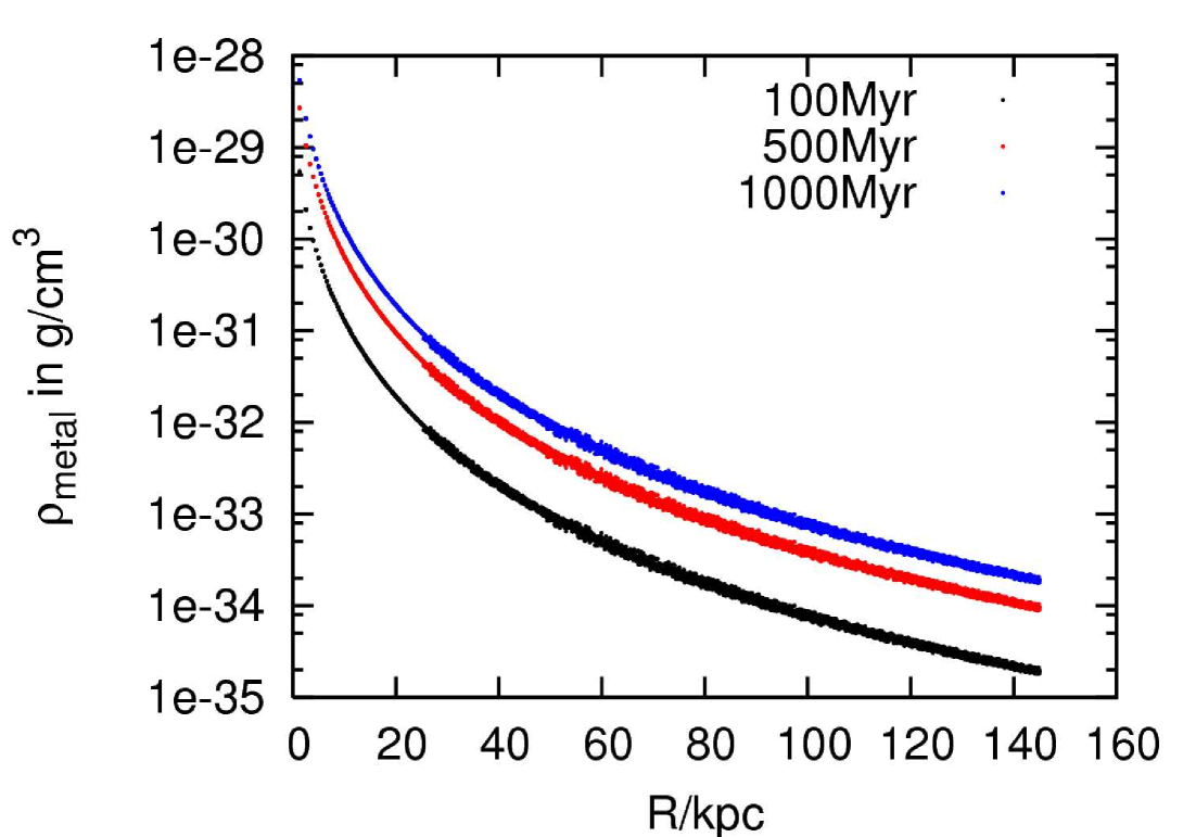
Figure 1: Evolution of the metal density profile in the case without bubbles. The metal density increases with time proportional to the light profile of the central galaxy. The injection rate is assumed to be constant in time. It is apparent that numerical mixing is very small. The noise increases at larger radii as the refinement levels go down.

Even after $1\,\textrm{Gyr}$ the 3 refinement levels can be seen in the profiles (where the “line” becomes thicker). Numerical velocities are of the order of $1\,\textrm{km}\,\textrm{s}^{-1}$ inside the grid and of $15\,\textrm{km}\,\textrm{s}^{-1}$ at the grid boundary.

3.2 Single pair of bubbles

In the next step, we produced a single pair of bubbles by evacuating two spherical regions of radius 10 kpc off-centre and on opposite sides of the cluster centre. The distance of the bubble centre from the cluster centre is 16 kpc. We studied the effect of this single pair of bubbles on the metal profile in the cluster. In particular, we wanted to compute how much mixing a single pair of bubbles can cause and what the long term fate of these bubbles is. Figures 2 to 3 show the results from this run.

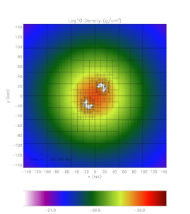
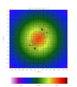
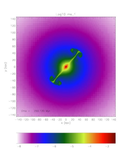
Figure 2: Simulation of a single bubble pair: Slice through the centre of the computational box showing the local gas density (left column) and the metal fraction (right column) at 60 Myr (top) and 250 Myr (bottom). The grid lines indicate the boundaries of the blocks. Each block contains $8^{3}$ computational cells.

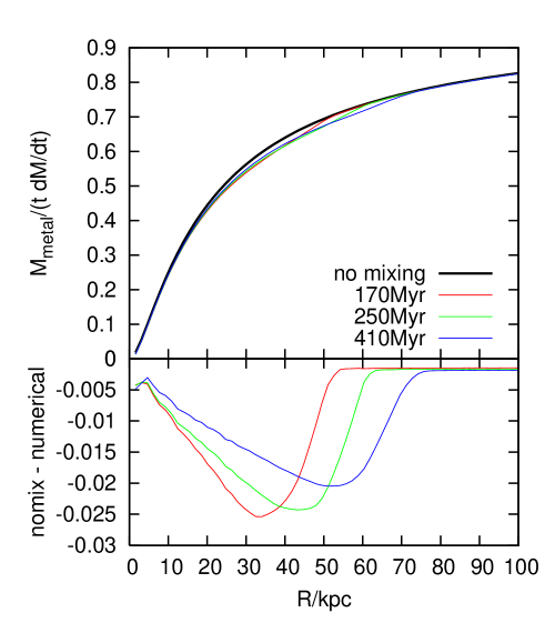
Figure 3: Normalised cumulative metal mass for the run with a single pair of bubbles. These masses are averages in shells centred on the cluster. The thick solid line shows the cumulative metal mass without mixing. The bottom panel shows the difference between cumulative mass with and without mixing.

As found in previous studies, the bubbles start to rise buoyantly and fragment. While rising, they uplift the metals from the centre and distribute them in their wake. Quite quickly the bubble fragments into a torus. Associated with this torus is a vortical flow that causes gas to ascend through the axis of the torus. Along the axis of the torus, metals seem to be transported rather fast. However, this metal spreading seems to be restricted to a narrow region around this direction. Spreading along other directions seems negligible. The effect is that the metals are spread out significantly along the axis of the bubbles leading to a very elongated metal distribution. Globally, the effect of a single pair of bubbles is not very significant (see cumulative metal mass profile in Fig. 3).

The bubbles do not continue to rise indefinitely and even after 1 Gyr they do not rise beyond 100 kpc from the centre. When they fragment, their rise velocity decreases. This can easily be seen by equating the drag force to the buoyance force, i.e.

$$\frac{4}{3}\pi r^{3}\rho g=\frac{\pi}{2}Cr^{2}\rho v^{2}\ ,$$ (8)

where $v$ is the terminal velocity, $\rho$ the density of the ambient medium, $g$ the gravitational acceleration, $r$ the radius of the bubble and $C$ a constant of order unity. This yields the terminal velocity

$$v^{2}=\frac{8rg}{3C}\ .$$ (9)

Thus, the rise velocity $\propto\sqrt{r_{\mathrm{bbl}}}$ (see e.g. Churazov et al. (2001)). The fragments form a mushroom-shaped plume, not unlike the radio structures observed in M87, and this structure covers a larger azimutal angle. There could be a certain radius where most metals are deposited.

Two effects can lead to a more isotropic mixing of metals: (i) ambient motions in the cluster that are triggered by galaxy motions and merger activity and (ii) a series of bubbles that are launched at changing locations in the cluster, for example by a precessing jet or by inhomogeneities of the accretion flow near the jet. In the next section, we investigate the second scenario.

3.3 Series of bubbles

In the next set of simulations, we look at the effect of a succession of bubbles that are generated at changing positions inside the cluster.

3.3.1 Distance of bubbles from cluster centre

One would expect that the starting position of the bubbles with respect to the central galaxy affects the amount of metals that can be uplifted from the galaxy. This is indeed the case as we see by comparing runs EVAC and DISTCTR. If bubbles start too far out, they cannot uplift a substantial amount of metals because most metals are injected mainly in the cluster centre (steep metal injection profile) as can be seen from Fig. 4.

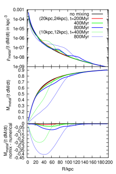
Figure 4: Evolution of the normalised metal density profile (top panel) and the normalised cumulative metal mass profile (metal mass inside $r$, middle panel). The bottom panel shows the difference between mixing and no mixing. This figure shows the impact of the launch position of the bubbles. We compare runs EVAC and DISTCTR.

In order to compare metal fraction, metal density and cumulative metal mass at different times, these quantities are normalised to $\dot{M}_{\mathrm{metal}}{}_{0}\cdot t$. From this we can conclude that the initial position of the bubbles with respect to the scale radius of the metal injection rate has an impact on the mixing efficiency of the bubbles. However, as the bubbles are produced by jets that are launched from supermassive black holes at the centre of the galaxy, the bubbles will never be inflated too far from the stars that produce the metals. While in principle the mixing efficiency depends on the initial position of the bubble, the nature of the bubbles will ensure that this will not cause great differences in the metal profiles. Our generic run has a distance of the bubble centre from the core of the cluster of $\sim 16$ kpc. In reality, bubbles occur at a broad range of distances from the centre. The list of known bubbles in Dunn et al. (2005) shows that the distances that we probe lie well within the observed ones.

3.3.2 Bubble size

Obviously, one important parameter is the size of the bubbles. In our standard scenario we chose a bubble radius of 10 kpc which is motivated by the sizes of some of the cavities observed in the X-ray surface brightness maps. For example, the cavities of the inner bubbles in Perseus have a radius of 13 kpc. To test the dependence of the transport efficiency on the bubble size, we compared our standard run with a bubble of twice its radius (8 times its volume). See Fig. 5 for the cumulative metal mass profiles. The main inference is that larger bubbles can carry metals out to larger distances. As can be seen in Fig. 5, after about 500 Myrs the large bubble ($r=20$ kpc) carries the metals out to a distance of about 50 kpc, while the 10 kpc bubble only lifts them to about 25 kpc.

The same trend is apparent from Fig. 6 which shows the normalised radial metal density profile for three different times. The main effect of the bubbles can be seen in the points elevated above the original line. In these cells, the metal density is enhanced because the bubbles have carried the metals to larger radii. It is evident that the larger bubbles are more efficient at transporting metals outwards.

This behaviour is not surprising because larger bubbles rise faster as we saw in Eq. (9). As the bubbles rise faster, they accelerate the metals in its wake to higher velocities and they travel further out until instabilities have broken them up such that they do not travel much further.

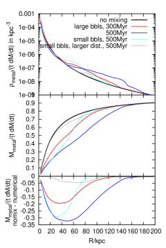
Figure 5: Evolution of the normalised metal density profile (top panel) and the normalised cumulative metal mass profile (metal mass inside $r$, middle panel). The bottom panel shows the difference between mixing and no mixing. Here we illustrate the impact of the initial bubble position and the initial bubble sizes. Shown are results from runs EVAC, DISTCTR and LARGEBBL.

3.3.3 Bubble frequency

Clearly, the efficiency with which bubbles can transport metals depends on the frequency with which bubbles are produced by the AGN. In the previous simulations, we employed a recurrence time of 50 Myr. For comparison, we ran a simulation with a recurrence time of 200 Myrs, all other parameters being the same as in run EVAC.

The difference in, both, radius up to which metals are carried and degree of deformation of cumulative metal mass profile can be seen in Fig. 7. After 800 Myrs, comparing the blue and grey lines reveals the difference between these two runs. The runs with a longer recurrence time leads to appreciably less mixing. A recurrence time that is four times longer, roughly leads to only about 1/3 as much mixing by the end of our simulation. Thus, the degree of mixing scales roughly with the frequency of bubble generation as one would expect.

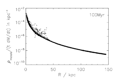
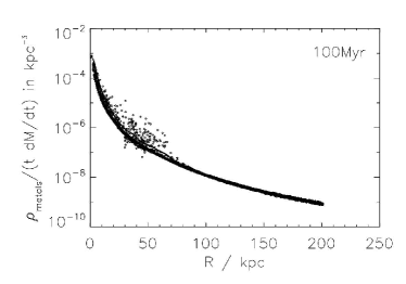
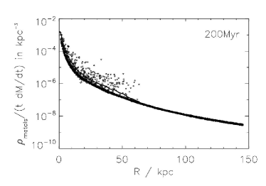
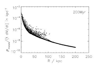
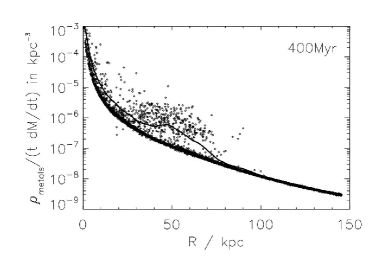
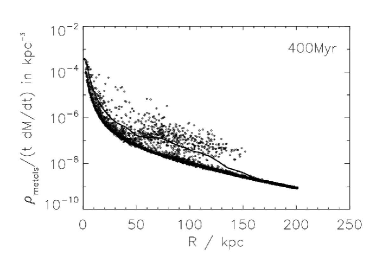
Figure 6: Normalised radial metal density profile for three different times. A random subset of cells is chosen (same weight for each radius). Metal density is normalised to $t\dot{M}_{\mathrm{metal}}{}_{0}$. Left column is for EVAC, right column for LARGEBBL. The main effect of the bubbles can be seen in the points elevated above the original line. In these cells, the metal density is enhanced because the bubbles have carried the metals to larger radii. It is apparent that the larger bubbles are more efficient at transporting metals outwards.

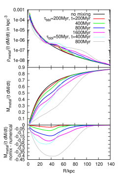
Figure 7: Evolution of normalised metal density profile (top panel) and and normalised cumulative metal mass profile (metal mass inside $r$, middle panel). The bottom panel shows the difference between mixing and no mixing. Comparison of two runs with different bubble evacuation timescale ($\tau_{\mathrm{bbl}}$) (runs EVAC and TAUBBL200). Different line styles and colours correspond to different times and runs, see legend. The black line is the prediction of what should happen without any mixing.

3.3.4 Comparison between evacuation and inflation method

In Fig. 8, we investigate the sensitivity of the metal profiles to the way we produce the bubbles. We generate the bubbles by either injecting hot gas into a number of computational cells or by removing gas mass from a spherical region of space while keeping the pressure constant. Reassuringly, the differences between the two methods are small. In the evacuation method the bubbles seem to be able to carry metals out a little bit further. Also the global effect (flattening of cumulative metal mass profile, see Fig. 8) is a bit stronger in the evacuation scenario. However, all properties concerning the transport of metals in the cluster are very similar in both runs. The evacuation method is computationally slightly cheaper because the timesteps during the inflation phase become quite small. Projections of the gas density, the X-ray surface brightness and the normalised metal density for different timesteps are shown in Fig. 9. Therefore, we produce the bubble by evacuation in all our other runs.

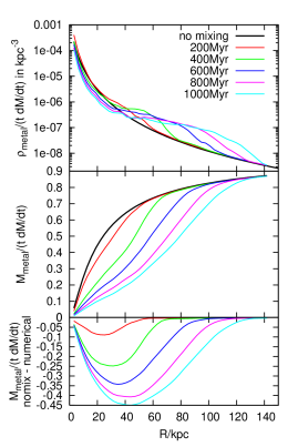
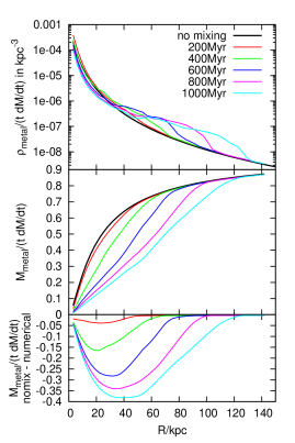
Figure 8: Evolution of the metal density profile (top panels) and the cumulative metal mass profile (metal mass inside $r$, middle panels). Both profiles are normalised to $t\dot{M}_{\mathrm{metal}}{}_{0}$. Different timesteps are colour-coded, see legend. Left is for bubble evacuation method, right for bubble inflation method. The black line is the prediction of what should happen without any mixing. The bottom panels show the difference between mixing and no mixing.

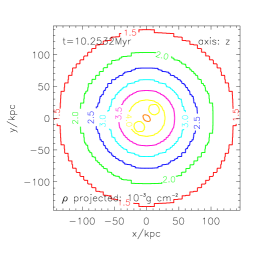
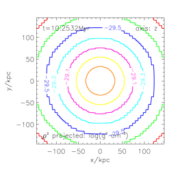
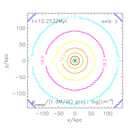
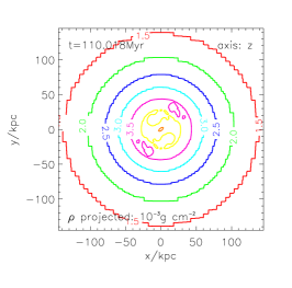
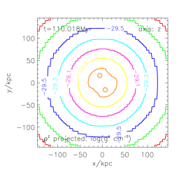
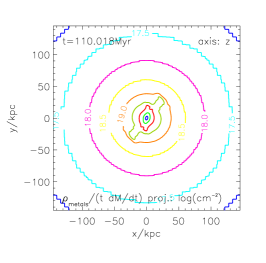
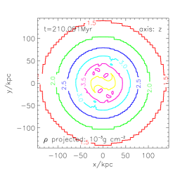
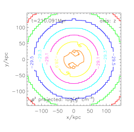
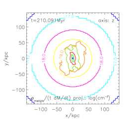
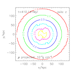
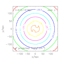
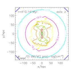
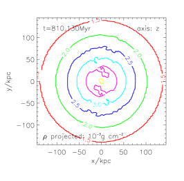
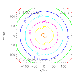
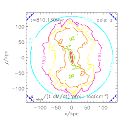
Figure 9: Projections of gas density (left column), $\rho^{2}$ (middle column) and normalised metal density (right column) for different timesteps (see label in each panel) for simulation EVAC. Projection is done along the $z$-axis.

3.3.5 Resolution test

In these kinds of simulations, it is essential to assess the errors caused by the spatial discretisation. We can compare runs EVAC and EVAC_HR which have an effective resolution of $192^{3}$ and $384^{3}$ zones respectively. The morphologies of the bubbles are very similar up to $250\,\textrm{Myr}$ and the cumulative mass profiles are practically indistinguishable. In Fig. 10, we show the normalised cumulative metal mass profiles for runs with resolutions of $192^{3}$ zones and $384^{3}$ zones. The resultant metal profiles suggest that the simulation have converged numerically.

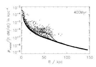
Figure 10: Left: Normalised cumulative metal mass profile (metal mass inside $r$) for run EVAC with an effective resolution of $192^{3}$ zones (top) and for run EVAC_HR with an effective resolution of $384^{3}$ zones (bottom). The upper line in both plots corresponds to the case without mixing. Right: Radial metal density profile normalised to $t\dot{M}_{\mathrm{metal}}{}_{0}$ for the $192^{3}$ run (top) and the $384^{3}$ run (bottom). All data corresponds to a time of 400 Myrs after the start of the AGN activity.

3.4 The case of Perseus

Having discussed a somewhat generic cluster model above, we now turn to the brightest X-ray cluster A426 (Perseus) that has been studied extensively with Chandra and XMM-Newton. Our simulations of the Perseus cluster show two things: (i) In the case of Perseus, the metal distribution is somewhat broader. This is a result of the greater pressure gradient in Perseus which leads to a greater buoyancy force and thus a higher velocity of the bubbles. (ii) We find that despite varying the initial positions of the bubbles, the resulting metal distribution remains fairly elongated and decidedly non-spherical.

Fig. 11 shows the local metal fraction at three different times in slices through the centre of the cluster. The left column is for the generic background cluster (EVAC) and right column for the simulation based on Perseus. For the Perseus model, the metal disribution is somewhat broader than in our generic model. However, all qualitative features discussed above for the generic model remain valid for the cluster based on Perseus.

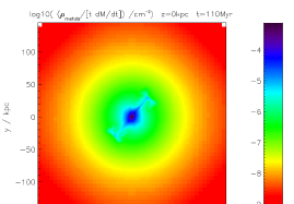
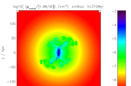
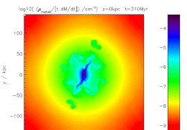
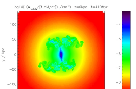
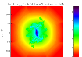
Figure 11: Slice through the computational box showing local metal fraction at three different times. Left column is for the generic background cluster (EVAC), and right column for the simulation based on Perseus (PERSEUS_50).

3.5 Estimate of diffusion constant

In this section, we wish to parametrise the transport of metals by computing an effective diffusion constant. We will begin by defining a cumulative metal mass profile

$$M_{\mathrm{metal}}(R)=\int\limits_{r<R}\rho_{\mathrm{metal}}(\vec{r})\mathrm{d}V$$ (10)

and the averaged metal density profile

$$\bar{\rho}_{\mathrm{metal}}(r)=\frac{1}{4\pi r^{2}}\frac{\partial M_{\mathrm{metal}}(r)}{\partial r}.$$ (11)

On the basis of these quantities, we can estimate a diffusion constant that can be compared with Rebusco et al. (2005). We start from the spherically symmetrical diffusion equation including the metal source term

$$\frac{\partial\bar{\rho}_{\mathrm{metal}}(r,t)}{\partial t}=\frac{\partial}{\partial r}D\frac{\partial}{\partial r}\bar{\rho}_{\mathrm{metal}}(r,t)+\dot{\rho}_{\mathrm{metal}}(r),$$ (12)

where $D$ is the diffusion constant, and $\dot{\rho}_{\mathrm{metal}}(r)$ is the metal source profile according to Eq. 4. Discretising this between the radii $R_{1}$ and $R_{2}$ (i.e. $\Delta R=R_{2}-R_{1}$ and $\bar{R}=(R_{1}+R_{2})/2$) and timesteps $t_{1}$ and $t_{2}$ ($\Delta t=t_{2}-t_{1}$ and $\bar{t}=(t_{1}+t_{2})/2$) yields

$$\frac{\bar{\rho}_{\mathrm{metal}}(\bar{R},t_{2})-\bar{\rho}_{\mathrm{metal}}(\bar{R},t_{1})}{\Delta t}=\dot{\rho}_{\mathrm{metal}}(\bar{R})+$$

$$D(\bar{R},\bar{t})\;\frac{\frac{\partial}{\partial r}\bar{\rho}_{\mathrm{metal}}(R_{2},\bar{t})-\frac{\partial}{\partial r}\bar{\rho}_{\mathrm{metal}}(R_{1},\bar{t})}{\Delta R},$$ (13)

where we have assumed that $D$ varies only slowly with radius, i.e. $D(R_{1},t)\approx D(R_{2},t)\approx D(\bar{R},t)$. Reordering yields

$$D(\bar{R},\bar{t})=$$

$$\Delta R\;\frac{\bar{\rho}_{\mathrm{metal}}(\bar{R},t_{2})-\bar{\rho}_{\mathrm{metal}}(\bar{R},t_{1})-\dot{\rho}_{\mathrm{metal}}(\bar{R})\,\Delta t}{\Delta t\;\left[\frac{\partial}{\partial r}\bar{\rho}_{\mathrm{metal}}(R_{2},\bar{t})-\frac{\partial}{\partial r}\bar{\rho}_{\mathrm{metal}}(R_{1},\bar{t})\right]}$$ (14)

For the runs described in the previous sections, we have computed the radial profiles of the diffusion constants in Fig. 12.

Figure 12: Diffusion coefficients for the runs EVAC (top left), INFL (top right), TAUBBL200, (middle left), DISTCTR (middle right), PERSEUS_50 (bottom left) and PERSEUS_200 (bottom right). The different curves denote different times.

4 Discussion

In our simulations, the dynamics of the ICM is entirely driven by underdense bubbles that are initially at rest and then start to rise by the action of buoyancy. This is clearly a simplified picture. In reality, these bubble are inflated by relativistic jets whose physics is still very poorly understood. Real AGN jets have a dynamics that can only be fully captured with special-relativistic MHD codes that need to resolve scales much below the scales resolved in our simulations.

However, bubbles such as those set up in our simulations are similar to the bubbles observed in galaxy clusters such as the Perseus cluster. The bubbles in Perseus and other clusters are nearly in pressure equilibrium with the ambient medium, they are nearly spherical and move subsonically through the ICM. Thus, we ignore the entire process that has led to the formation of these bubbles and focus solely on the buoyancy-driven motions of the bubbles.

There have been some attempts to simulate the inflation of the bubbles by a jet and assess its consequences for the ICM. Omma et al. (2004) simulate the effect of slow jets on a cool core in a galaxy cluster. Simulations by Vernaleo & Reynolds (2006) show that jets launched in a hydrostatic cluster fail to heat the cluster on long time scales because the jet forms a low-density channel through which the material can flow freely, carrying its energy out of the cooling core.

If bubbles in a hydrostatic cluster are launched repeatedly at the same position, the resulting metal distribution becomes very aspherical and elongated along the axis of the bubble. If, however the bubbles are launched at changing positions, the metal distribution is somewhat isotropised. However, as is apparent e.g. from Fig. 11, even when we vary the bubble position within a cone of $\sim 30\deg$, the resulting metal distribution remains elongated and non-spherical. Thus, if the metal distribution should turn out to be spherical, this would necessitate additional motions caused for example by mergers or by stirring by galaxies in order to isotropise the metals.

In real clusters, the ICM is not in hydrostatic equilibrium and can show strong motions. Galaxies that fly through the cluster produce motions and turbulence. Merger activity can stir the ICM even more violently. These motions will all contribute to dispersing the metals throughout the ICM. Moreover, density anisotropies can cause the bubbles to move away from the axis of the AGN jet, as the bubbles follow the local density gradient. Indeed, in quite a few clusters, most famously in M87, the bubbles are widely dispersed through the cluster and do not trace the alleged axis of the AGN jet. Heinz et al. (2006) have performed three-dimensional adaptive-mesh simulations of jets situated at the centre of a cluster drawn from a cosmological simulation. These simulations show that cluster inhomogeneities and large-scale flows have a significant impact on the morphology of the bubbles. Moreover, these motions help to prevent the formation of channels along the bubbles axes as found by Vernaleo & Reynolds (2006).

The diffusion coefficients inferred from our simple experiments lie at values of around $\sim 10^{29}$ cm²s^-1 at a radius of 10 kpc. Right at the centre, they rise to about $\sim 10^{31}$ cm²s^-1 and fall to about $\sim 10^{25}$ cm²s^-1 at a radius of 100 kpc. Modulo a factor of a few, the coefficients for all runs lie around these values. Differences are induced by the bubble sizes, the initial positions, the recurrence times and the pressure profile in the cluster. Interestingly, the runs modelled on the Perseus cluster yield diffusion coefficients that agree very well with those estimated by assuming a simple diffusion model (see Rebusco et al. (2005)). As we do not take into account motions that may have been induced by mergers etc., the values for the diffusion coefficients constitute lower limits on the real values. Thus, we can conclude that AGN-induced motions are sufficient to explain the broad abundance peaks in clusters. It is also striking that the diffusion coefficients fall so steeply with radial distance from the centre. Over two decades in radius they decrease by almost 10 orders of magnitude. Very approximately, they fall like $r^{-5}$. This strong radial dependence of the transport efficiency is, partially, a result of the three-dimensional nature of the bubble-induced motions, i.e. uplifted metals are diluted over the entire radial shell. A second effect is the decaying “lift” power of the bubbles as they rise. The bubbles accelerate only at the beginning of their ascent through the cluster. However, very quickly instabilities set in that slow down the bubble until it finally comes to a halt at about 100 kpc from the centre. The maximal lift power is attained when the bubbles are still intact and have their largest velocity. This occurs at radii of about 20 kpc - 30 kpc, and this coincides with peaks in the diffusion coefficient as can be seen from Fig. 12, particularly for runs EVAC and PERSEUS_50.

Finally, we may add that if hydrodynamic instabilities are suppressed by magnetic fields or viscous forces, for example, the bubbles would stay intact for longer and could rise to greater distances thus also enhancing the diffusion coefficients at larger radii.

5 Summary

In a series of numerical experiments, we have performed a systematic study on the effect of bubble-induced motions on metallicity profiles in clusters of galaxies. In particular, we have studied the dependence on the bubble size and positions, the recurrence times of the bubbles, the way these bubbles are inflated and the underlying cluster profile.

On the basis of our 3D hydro simulations, we wish to make the following main points:

• Larger bubbles lead to mixing to larger radii. For realistic parameters and in the absence of stabilising forces, bubbles hardly move beyond distances of 150 kpc from the centre.

• Mixing scales roughly with bubble frequency.

• The metal distribution is not sensitive to the way of how bubbles are inflated.

• In hydrostatic cluster models, the resulting metal distribution is very elongated along the direction of the bubbles. Anisotropies in the cluster and/or ambient motions are needed if the metal distribution is to be spherical.

• The diffusion coefficients inferred from our simple experiments lie at values of around $\sim 10^{29}$ cm²s^-1 at a radius of 10 kpc.

• The runs modelled on the Perseus cluster yield diffusion coefficients that agree very well with those inferred from observations (see Rebusco et al. (2005)).

References

- Aguirre et al. (2001) Aguirre A., Hernquist L., Schaye J., Katz N., Weinberg D. H., Gardner J., 2001, ApJ, 561, 521
- Arnaud et al. (1992) Arnaud M., Rothenflug R., Boulade O., Vigroux L., Vangioni-Flam E., 1992, A&A, 254, 49
- Basson & Alexander (2003) Basson J. F., Alexander P., 2003, MNRAS, 339, 353
- Bîrzan et al. (2004) Bîrzan L., Rafferty D. A., McNamara B. R., Wise M. W., Nulsen P. E. J., 2004, ApJ, 607, 800
- Böhringer et al. (2004) Böhringer H., Matsushita K., Churazov E., Finoguenov A., Ikebe Y., 2004, A&A, 416, L21
- Brüggen & Kaiser (2002) Brüggen M., Kaiser C. R., 2002, Nature, 418, 301
- Brüggen et al. (2002) Brüggen M., Kaiser C. R., Churazov E., Enßlin T. A., 2002, MNRAS, 331, 545
- Brighenti & Mathews (2006) Brighenti F., Mathews W. G., 2006, ApJ, 643, 120
- Brüggen (2002) Brüggen M., 2002, ApJ, 571, L13
- Brüggen & Kaiser (2001) Brüggen M., Kaiser C. R., 2001, MNRAS, 325, 676
- Brüggen et al. (2005) Brüggen M., Ruszkowski M., Hallman E., 2005, ApJ, 630, 740
- Carilli & Taylor (2002) Carilli C. L., Taylor G. B., 2002, ARA&A, 40, 319
- Chandrasekhar (1961) Chandrasekhar S., 1961, Hydrodynamic and Hydromagnetic Stability. Dover
- Churazov et al. (2001) Churazov E., Brüggen M., Kaiser C. R., Böhringer H., Forman W., 2001, ApJ, 554, 261
- Churazov et al. (2003) Churazov E., Forman W., Jones C., Böhringer H., 2003, ApJ, 590, 225
- Churazov et al. (2004) Churazov E., Forman W., Jones C., Sunyaev R., Böhringer H., 2004, MNRAS, 347, 29
- Cora (2006) Cora S. A., 2006, MNRAS, 368, 1540
- Croton et al. (2006) Croton D. J., Springel V., White S. D. M., De Lucia G., Frenk C. S., Gao L., Jenkins A., Kauffmann G., Navarro J. F., Yoshida N., 2006, MNRAS, 365, 11
- Dalla Vecchia et al. (2004) Dalla Vecchia C., Bower R. G., Theuns T., Balogh M. L., Mazzotta P., Frenk C. S., 2004, MNRAS, pp 507–+
- De Grandi et al. (2004) De Grandi S., Ettori S., Longhetti M., Molendi S., 2004, A&A, 419, 7
- De Grandi & Molendi (2001) De Grandi S., Molendi S., 2001, ApJ, 551, 153
- De Lucia et al. (2004) De Lucia G., Kauffmann G., White S. D. M., 2004, MNRAS, 349, 1101
- De Young (2003) De Young D. S., 2003, MNRAS, 343, 719
- Domainko et al. (2006) Domainko W., Mair M., Kapferer W., van Kampen E., Kronberger T., Schindler S., Kimeswenger S., Ruffert M., Mangete O. E., 2006, A&A, 452, 795
- Dunn et al. (2005) Dunn R. J. H., Fabian A. C., Taylor G. B., 2005, MNRAS, 364, 1343
- Finoguenov et al. (2002) Finoguenov A., Matsushita K., Böhringer H., Ikebe Y., Arnaud M., 2002, A&A, 381, 21
- Fryxell et al. (2000) Fryxell B., Olson K., Ricker P., Timmes F. X., Zingale M., Lamb D. Q., MacNeice P., Rosner R., Truran J. W., Tufo H., 2000, ApJS, 131, 273
- Fukazawa et al. (2000) Fukazawa Y., Makishima K., Tamura T., Nakazawa K., Ezawa H., Ikebe Y., Kikuchi K., Ohashi T., 2000, MNRAS, 313, 21
- Heinz et al. (2006) Heinz S., Brüggen M., Young A., Levesque E., 2006, ArXiv Astrophysics e-prints
- Matsushita et al. (2002) Matsushita K., Belsole E., Finoguenov A., Böhringer H., 2002, A&A, 386, 77
- Mushotzky et al. (1996) Mushotzky R., Loewenstein M., Arnaud K. A., Tamura T., Fukazawa Y., Matsushita K., Kikuchi K., Hatsukade I., 1996, ApJ, 466, 686
- Omma et al. (2004) Omma H., Binney J., Bryan G., Slyz A., 2004, MNRAS, 348, 1105
- Owen & Ledlow (1997) Owen F. N., Ledlow M. J., 1997, ApJS, 108, 41
- Rebusco et al. (2005) Rebusco P., Churazov E., Böhringer H., Forman W., 2005, MNRAS, 359, 1041
- Renzini et al. (1993) Renzini A., Ciotti L., D’Ercole A., Pellegrini S., 1993, ApJ, 419, 52
- Reynolds et al. (2002) Reynolds C. S., Heinz S., Begelman M. C., 2002, MNRAS, 332, 271
- Reynolds et al. (2005) Reynolds C. S., McKernan B., Fabian A. C., Stone J. M., Vernaleo J. C., 2005, MNRAS, 357, 242
- Roediger & Brueggen (2005) Roediger E., Brueggen M., 2005, ArXiv Astrophysics e-prints
- Roediger et al. (2006) Roediger E., Brueggen M., Hoeft M., 2006, ArXiv Astrophysics e-prints
- Ruszkowski et al. (2004) Ruszkowski M., Brüggen M., Begelman M. C., 2004, ApJ, 611, 158
- Schindler et al. (2005) Schindler S., Kapferer W., Domainko W., Mair M., van Kampen E., Kronberger T., Kimeswenger S., Ruffert M., Mangete O., Breitschwerdt D., 2005, A&A, 435, L25
- Schmidt et al. (2002) Schmidt R. W., Fabian A. C., Sanders J. S., 2002, MNRAS, 337, 71
- Sijacki & Springel (2006) Sijacki D., Springel V., 2006, MNRAS, 371, 1025
- Tamura et al. (2004) Tamura T., Kaastra J. S., den Herder J. W. A., Bleeker J. A. M., Peterson J. R., 2004, A&A, 420, 135
- Tornatore et al. (2004) Tornatore L., Borgani S., Matteucci F., Recchi S., Tozzi P., 2004, MNRAS, 349, L19
- Tozzi et al. (2003) Tozzi P., Rosati P., Ettori S., Borgani S., Mainieri V., Norman C., 2003, ApJ, 593, 705
- Vernaleo & Reynolds (2006) Vernaleo J. C., Reynolds C. S., 2006, ApJ, 645, 83