The Axis of Evil revisited

Abstract

In light of the three-year data release from WMAP we re-examine the evidence for the “Axis of Evil” (AOE). We discover that previous statistics are not robust with respect to the data-sets available and different treatments of the galactic plane. We identify the cause of the instability and implement an alternative “model selection” approach. A comparison to Gaussian isotropic simulations find the features significant at the 94-98% level, depending on the particular AOE model. The Bayesian evidence finds lower significance, ranging from “substantial” at $\Delta(\ln E)\sim 1.4$, to no evidence for the most general AOE model.

1 Introduction

The Wilkinson Microwave Anisotropy Probe (WMAP) has produced spectacular high resolution all-sky observations of the Cosmic Microwave Background (CMB), which have bolstered the case for the $\Lambda$CDM concordance cosmological model (Spergel et al., 2003, 2006). After the release of the first-year results (Bennett et al., 2003) there was a flurry of studies into the Gaussianity and statistical isotropy of the data, as these are fundamental predictions of inflation theories. Reports of something awry have been obtained using a variety of techniques (e.g., Park (2004); Eriksen et al. (2004a); Hansen et al. (2004); Donoghue & Donoghue (2005); Land & Magueijo (2005a); Hansen et al. (2004); Eriksen et al. (2004b); Vielva et al. (2004)). In this paper we focus on anomalies in the largest scale modes, after it was first noted that the quadrupole ($\ell=2$) and octopole ($\ell=3$) appeared to be correlated (de Oliveira-Costa et al., 2004), and their power is suspiciously low. Much work has focussed on the alignment and “planarity” of these two multipoles (Copi et al., 2006; Schwarz et al., 2004; Ralston & Jain, 2004); but in Land & Magueijo (2005b) it was seen that the alignment actually extends to the four multipoles $\ell=2-5$, along the axis $(b,l)\approx(60,-100)$. This feature has been dubbed the “axis of evil” (AOE).

To be more precise the AOE expression has come to signify various different things. Generally it is intended to denote any form of statistical anisotropy, i.e., a feature in the CMB fluctuations which picks a preferred direction. This can be realized in many ways e.g., multipole planarity (the dominance of $m=\pm\ell$ modes along the preferred axis), or a more general form of $m$-preference. In this respect it must be said that while everyone agrees on the presence of the “axis of evil” in the data, its extent is still debated. The expression is also sometimes associated with the low power in the low $\ell$s. This is quite inappropriate: while low power may be related to the AOE (see Land & Magueijo (2006)) there is nothing “axial” or anisotropic in a power spectrum anomaly per se.

There are two possible fault lines in the analysis leading to the “axis of evil” effect. The first concerns the integrity of the data itself, i.e., contamination from noise, systematics and foregrounds. Comparison between the first-year (WMAP1) and third-year (WMAP3) data releases shows that the raw data has hardly changed on large scales. However there are several “all-sky” renditions of the data and these do lead to significant disparities: in this paper we show that this is true regarding the intensity of the AOE, so that discussions should emphasise not so much 1st V’s 3rd year data, but the various treatments of the galactic plane region.

The second fault line concerns the “meaning” of the detection, and by this we mean the robustness of the statistics used, and whether there is support for planarity or more general $m$-preference. The frequentist formalism provides no clean way to penalise for extra parameters or to weigh-up the detections against each other, or the null hypothesis. Instead simulations are used to assess how likely it is to get such a feature in a Gaussian statistcally isotropic (SI) CMB sky, but selection effects (by which we mean the tuning of the statistic or model to the data) are hard to account for. Here the confrontation of Bayesianism and frequentism becomes a very practical matter.

We carry out this project as follows. In Section 2 we re-examine the original frequentist AOE results for various renditions of the WMAP1 and WMAP3 data, and we discuss further the limitations of the original frequentist method, such as its lack of robustness, at least with regards to $m$-preference AOE (as opposed to “planarity”). In Section 3 we follow a model comparison approach, and find that this is much more robust when confronted with the different data-sets. Further we compare the evidence for the models; planarity and more complex $m$-preference. In Section 4 we summarise and discuss the results.

2 Instabilities of the frequentist statistics

	$\ell=2$		$\ell=3$		$\ell=4$		$\ell=5$		Mean
Map	$(b,l)$	m	$(b,l)$	m	$(b,l)$	m	$(b,l)$	m	inter-$\theta$
LILC1	(0.9, 156.7)	0	(63.0, -126.9)	3	(56.7, -163.7)	2	(48.6, -94.7)	3	51.4
TOH1	(58.5, -102.9)	2	(62.1, -120.6)	3	(57.6, -163.3)	2	(48.6, -93.4)	3	22.4
TOH3	(76.5, -134.0)	2	(27.0, 51.9)	1	(35.1, -130.6)	1	(47.7, -94.7)	3	53.8
WMAP3	(2.7, -26.5)	0	(62.1, -122.6)	3	(34.2, -131.2)	1	(47.7, -96.0)	3	53.7

Table 1: The ${\bf n}_{\ell}$ axes, in galactic coordinates $(b,l)$, and $m$ that maximise (2) for the multipoles $\ell=2-5$, for various all-sky renditions of the first and third-year WMAP data. Note the low mean inter-angle values for the TOH1 map, which indicate a strong correlation between the multipoles (it i.e., AOE). The dicontinuous nature of the statistic causes the results to vary widely.

To assign an axis to each multipole,  de Oliveira-Costa et al. (2004) proposed the following statistic:

$$q_{\ell}=\max_{\bf n}\left[\sum_{m}m^{2}|a_{\ell m}({\bf n})|^{2}\right],$$ (1)

where the $a_{\ell m}$s are computed in the frame with ${\bf z}$-axis in direction ${\bf n}$. This selects the frame dominated by the planar $m=\pm\ell$ modes.

In Land & Magueijo (2005b) we generalized this statistic to allow for any $m$ domination, i.e., not restricting ourselves to planar configurations, with the statistic:

$$r_{\ell}=\max_{m{\bf n}}\left[\frac{C_{\ell m}({\bf n})}{\sum|a_{\ell m^{\prime}}|^{2}}\right],$$ (2)

where $C_{\ell 0}({\bf n})=|a_{\ell 0}|^{2}$, and $C_{\ell m}({\bf n})=2|a_{\ell m}|^{2}$ for $m>0$ (notice that 2 modes contribute for $m\neq 0$), for the $a_{\ell m}$s computed in the frame with ${\bf z}={\bf n}$. This produces three important quantities for each multipole: the direction ${\bf n}_{\ell}$, the “shape” $m_{\ell}$, and the ratio $r_{\ell}$ of the multipole’s power absorbed by the mode $m_{\ell}$ in the direction ${\bf n}_{\ell}$.

We extend the work of Land & Magueijo (2005b) by applying this statistic to the following data-sets:

$\bullet$ The WMAP mission (Bennett et al., 2003) produced full sky CMB maps from ten differencing assemblies (DAs). They also produced an “internal linear combination” (ILC) map. This assumes no external information about the foregrounds and combines smoothed frequency maps with weights chosen to minimize the rms fluctuations, using separate sets of weights for 12 disjoint sky regions. In the first-year data release the WMAP collaboration advised that the ILC map be used only as a visual tool. However, for the third-year release a thorough error analysis of the ILC map was performed, and a bias correction implemented (Hinshaw et al., 2006). The resulting third-year ILC map (herein WMAP3) is expected to be clean enough on scales $\ell\mathrel{\hbox to0.0pt{\raise 2.20013pt\hbox{$<$}\hss}{\lower 2.20013pt\hbox{$\sim$}}}10$ to be used without a mask. WMAP data is available from http://lambda.gsfc.nasa.gov.

$\bullet$ Third-party maps include those of Tegmark et al. (2003), who produced their own ILC map. Like above, an “internal” method is employed assuming only a black-body spectrum for the CMB, but now the weights depend on scale (in harmonic space) as well as galactic latitude. This is advantageous because different sources of contamination dominate at different scales - foregrounds at large scales, and noise at smaller scales. As well as the cleaned map, a Wiener filtered map is produced that, through a comparison with the WMAP best estimates of theoretical $C_{\ell}$, adjusts the power of the map so to suppress noisy fluctuations. We use their first (TOH1) and third-year (TOH3) cleaned-maps, all available from www.hep.upenn.edu/ max/wmap.html.

$\bullet$ In an anlaysis of the ILC map-making method, Eriksen et al. (2004) proposed a faster algorithm for the computation of the weights, that employs Lagrangian multipliers to linearize the problem. Although this produces identical results to that of the WMAP team, and is indeed the method employed by the WMAP collaboration for their third-year map, the authors applied it to the first-year data using slightly different regions, thus producing a slightly different ILC map (herein LILC1), available at http://lambda.gsfc.nasa.gov.

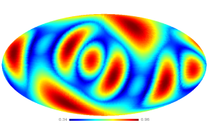
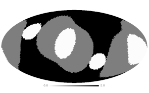
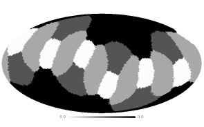
Figure 1: The power ratio $R_{\ell}({\mathbf{n}})$ in the dominating $m$ mode (above), and the $m$ value (below) for the quadrupole (left) and octopole (right). The “axis of evil” statistic in (2) searches for the hottest spot in these maps. We can see the close calls that cause the results to vary widely in Table 1. Plotted in galatic coordinates and Mollweide projection.

There are of course the original frequency maps, which require a mask. However, for the task of assessing statistical isotropy we require full sky information, and thus we only employ these ILC maps.

In Table 1 we list the results obtained with frequentist AOE statistic (2) for the various data-sets. It is clear that this statistic is not robust - very similar maps can find very different results as indicated by the final column. The expected inter-angle for isotropic axes is 1 radian ($\sim 57^{\circ}$), thus a mean of $\sim 22^{\circ}$ is remarkably low and a comparison to simulations puts this at the 99.9% confidence level (Land & Magueijo, 2005b). However, this result only holds for two of the maps, and a small fluctuation in just one multipole makes the ${\bf n}_{\ell}$ jump elsewhere. This highlights one weakness of this statistic - its discontinuous nature.

In Fig. 1 we visualize how “close calls” may arise, explaining the discontinuities of the results in Table 1. For the quadrupole and octopole of the TOH1 map, we plot the power ratio at the position ${\bf n}$

$$R_{\ell}({\mathbf{n}})=\max_{m}\frac{C_{\ell m}({\bf n})}{\sum|a_{\ell m^{\prime}}|^{2}}.$$ (3)

Thus the “axis of evil” statistic (2) picks out ${\bf n}_{\ell}$ as the position of the hottest spot from these maps (note the degeneracy between $m=1,2$ for $\ell=2$ - we avoid this in practice by taking just the $m=2$ solution). Below the $R_{\ell}$ maps we plot the associated $m$ picked by $R_{\ell}$ for a given ${\mathbf{n}}$. We can now diagnose the instabilities in Table 1, by identifying close calls in the competition for the hottest spot. For the quadrupole the $m=0$ and $m=2$ modes, and for the octopole the $m=1$ and $m=3$ modes are fighting a close battle. The overall mean inter-angle (which measures the strength of the AOE) depends closely on this battle, and thus the instability of this statistic. We should stress that the instabilities identified here do not seem to plague statistics for planarity (Magueijo & Sorkin, 2006).

3 Model Comparison

The instabilities discovered appear to be cured by a model comparison treatment, which allows for an evaluation of the evidence for $m$-preference in $\ell=2-5$, over simple planarity for $\ell=2,3$. Rather than computing a statistic from the maps (e.g., the mean inter-angle between the ${\mathbf{n}}$ for the various $\ell$), the idea is to assess the “evidence” for a model encoding $m$-preference or planarity, compared to the base model of statistical isotropy. We first outline the general formalism.

Let ${\cal L}$ be the likelihood of the data given a model, and $k$ the number of parameters of this model. The parameters should be tuned so to maximize the likelihood, or equivalently, to minimize the information in the data given the theory (defined as $I(D|T)=-\ln({\cal L})$). However the real evidence should refer to the information in the data and the theory: $I(D\cap T)=I(D|T)+I(T)$, where the information in the theory, $I(T)$, provides a penalization related to the number of parameters. This matter is behind the “Occam’s razor” rationale (Magueijo & Sorkin, 2006), and the information criteria (Liddle, 2004). According to the Aikaike informaiton criteria (AIC), the information in a theory is simply the number of parameters, $k$. In fact, we will use a more accurate form, which is especially important for small sample size, $I^{AIC}=k+\frac{k(k+1)}{N-k-1}$, where $N$ is the number of data points being fit (Burnham & Anderson, 2006).

An alternative approach to the problem of penalization is to compute the Bayesian evidence,

$$E=\int{\cal L}(D|\theta,M)\;\Pi(\theta){\rm d}\theta=P(D|M),$$ (4)

where $\Pi$ are the priors on the parameters $\theta$ for the model in question (see e.g., Trotta (2005) for a review). Bayes theorem tells us how this is related to the probability of a model $P(M|D)$, and it provides an effective penalization by computing the average of the likelihood over this expanded parameter space. As an approximation to the logarithm of the Bayes factor, $B\equiv E_{1}/E_{0}$, we will compute the Bayesian information criteria (BIC), $I^{BIC}=\frac{k}{2}\ln N$ (confusingly this is not actually related to information-theoretic methods).

The evidence $H$ for a theory $T_{1}$ is then defined as the decrease in the information of data and theory when it is compared with a null hypothesis $T_{0}$:

$$H = I(D\cap T_{0})-I(D\cap T_{1})$$ (5)

$$\equiv H_{f}-H_{p},$$

where $H_{f}$ measures the improvement in the fit $H_{f}=\ln({\cal L}_{1})-\ln({\cal L}_{0})$, and $H_{p}$ is the extra penalization we have in our new theory.

In the language of the Jeffreys’ scale (Jeffreys, 1961; Liddle et al, 2006) $\ln(B)$, or $H$, between 1 and 2.5 signals substantial evidence, between 2.5 and 5 signals strong evidence, and “decisive” evidence requires $\ln(B)>5$. However, for these rules of thumb to apply to the IC methods, various conditions should be met. For example the AIC assumes Gaussianity of the likelihood with respect to the parameters, while the BIC assumes independent identically distributed data points. We will therefore compare these results to those from statistically isotropic Gaussian simulations, in Section 3.3. We will also compute the Bayes factor, for comparison with the BIC approximation, and the frequentist results.

Data-set	($b$	$\quad l$)	$\epsilon$	$H_{f}$	$H^{AIC}$	$H^{BIC}$	$\ln B$
LILC1	63	-120	.042	6.51	2.01	2.78	1.36
TOH1	61	-113	.032	7.48	2.98	3.75	1.85
TOH3	74	-129	.018	6.97	2.47	3.24	1.27
WMAP3	64	-123	.043	6.49	1.99	2.76	1.32

Table 2: The maximum likelihood improvement, $H_{f}$, and best-fitting parameters for the planarity model (i.e., 3 extra parameters), from various all-sky renditions of the WMAP data. We consider the evidence from AIC and BIC methods as well as the Bayes factor ($\ln B\equiv\Delta\ln E$).

3.1 Planarity model

It was shown in Magueijo & Sorkin (2006) that the planarity of the $\ell=2,3$ multipoles is supported by a Bayesian analysis. The model used to assess the evidence for planarity is based on the diagonal covariance matrix:

$${\langle|a_{\ell m}|^{2}\rangle}({\bf n})=c_{\ell}\left(\delta_{\ell|m|}+\epsilon(1-\delta_{\ell|m|})\right)$$ (6)

where ${\bf n}$ and $\epsilon$ are the free parameters of the model (in addition to $c_{\ell}$ that is common with the isotropic model, but of a different value), with $\epsilon\leq 1$. We use the same $\epsilon$ and ${\bf n}$ for both multipoles, so that $k=3$, $N=12$, $H^{AIC}_{p}=4.5$, and $H^{BIC}_{p}=3.73$. In Table 2 we list the parameter values that maximize the likelihood, together with $H_{f}$ and $H$ following the AIC and BIC methods.

We also compute the Bayesian evidence and record $\ln(B)$ in Table 2. We do this via brute force integration, and for the base model ($\left<|a_{\ell m}|^{2}\right>=c_{\ell}$) we use a uniform prior on $c_{\ell}$; $0\leq c_{\ell}\>\ell(\ell+1)/(2\pi)\leq 3000\mu K^{2}$. For the planarity model we use uniform priors on $\epsilon\in[0,1]$, and on $c_{\ell}$; $0\leq c_{\ell}\>\ell(\ell+1)/(2\pi)\leq(2\ell+1)\times 3000\mu K^{2}$, with the further constraint $\bar{c}_{\ell}\>\ell(\ell+1)/(2\pi)\leq 3000\mu K^{2}$ where $\bar{c}_{\ell}$ is the average $\bar{c}_{\ell}=\sum_{m}\left<|a_{\ell m}|^{2}\right>/(2\ell+1)$.

As before (Magueijo & Sorkin, 2006) we find that variations between different galactic plane treatments lead to only small variation in $H_{f}$. However, different evidence measures reach different conclusions. All the measures find at least substantial evidence for the planarity model, however the AIC and BIC appear to significantly overestimate this evidence compared to the $\ln(B)$ result. We refer to Section 3.3 for a frequentist assessment of significance, through an analysis of $H_{f}$ from simulations.

3.2 General $m$-preference model

Using the same formalism we now revisit the debate on the extent of the AOE, i.e., $m$-preference as opposed to planarity. In the Bayesian formalism the matter can be addressed by replacing the the covariance matrix (6) by

$${\langle|a_{\ell m}|^{2}\rangle}({\bf n})=c_{\ell}(\delta_{m^{\prime}|m|}+\epsilon(1-\delta_{m^{\prime}|m|}))$$ (7)

where ${\bf n}$, $\epsilon$ and $m^{\prime}(\ell)$ are the free parameters of the model, with $\epsilon\leq 1$. We find that if we analyze each $\ell$ separately we rediscover the instabilities reported in Section 2. In Table 3 we take TOH1 for definiteness, and present the winning $m^{\prime}$, its associated $(b,l)$ and $H_{f}$; and also the runner up in cases where we get close calls in maximising $H_{f}$. We see that the Bayesian analysis, in this set up, merely confirms the $\ell=2$, $m^{\prime}=0,2$ and the $\ell=4$, $m^{\prime}=0,2$ instabilities.

However, a totally new perspective into these instabilities now makes itself known. $H_{f}$ only becomes the real evidence $H$ after it is degraded by the penalization $H_{p}$, related to the number of parameters of the model. If we allow each $\ell$ to choose its own parameters then the overall $H_{f}$ is large (the sum total) but the penalization is prohibitive as each multipole has 3 parameters. Thus in optimizing $H$ we wish to reduce the number of parameters by always seeking a common axis ${\bf n}$ for all $\ell$ in (7). This immediately removes the instabilities found in the frequentist formalism, by effectively penalizing for jumping between close calls, when one choice leads to a better common set of parameters.

$\ell$	$m^{\prime}$	($b$	$\quad l$)	$\epsilon$	$H_{f}$
2	0	6	157	0.027	3.47
2	2	59	-103	0.030	3.09
3	3	62	-120	0.025	5.06
4	2	58	-163	0.041	5.07
4	0	43	-98	0.043	4.02
5	3	49	-93	0.026	7.65

Table 3: The maximum likelihood improvement, $H_{f}$, for a dominating $m$-mode model in the TOH1 map, where each multipole can select its own axis, $\epsilon$, and $m^{\prime}$. Where there is a close call, the runner up $m^{\prime}$ is also listed.

Take for example $\ell=2$. We have that $m^{\prime}=0,2$ are close competitors in the optimization of $H_{f}$; however only $m^{\prime}=2$ picks an axis that is roughly aligned with the preferred axis for the other multipoles. So only $m^{\prime}=2$ permits a large saving in $H_{p}$ ($H_{p}=2$ per axis, using, say, the AIC) with only small deterioration in $H_{f}$. An instability would only arise if $m^{\prime}=0$ improved $H_{f}$ by an extra 2 when compared with $m^{\prime}=2$. The penalization forces the multipoles to chose common parameters, at the risk of decreasing the fit a little. Thus, in order to maximize $H$—and not only $H_{f}$—we should select a common ${\bf n}$ for $\ell=2-5$, and the complete result (for the same data-set) is presented in Table 5.

$\ell$	$m^{\prime}$	($b$	$\quad l$)	$\epsilon$	$H_{f}$
2	2	49	-96	0.052	2.33
3	3	49	-96	0.108	2.01
4	0	49	-96	0.058	3.21
5	3	49	-96	0.028	7.34
2-5	—	49	-96	——	14.89

Table 4: The maximum likelihood improvement, $H_{f}$, for a dominating $m$-mode in the TOH1 map, where each multipole can select its own $\epsilon$ and $m^{\prime}$, but a common favoured axis is found.

Data-set	($b$	$\quad l$)	$\epsilon$	$m$’s	$H_{f}$	$H^{AIC}$	$H^{BIC}$	$\ln B$	$\ln B_{23}$
LILC1	48	-100	.077	2303	11.46	2.13	-0.67	-1.43	-0.17
TOH1	49	-96	.051	2303	14.54	5.21	2.41	0.80	0.11
TOH3	48	-97	.073	2303	11.57	2.24	-0.56	-1.15	-0.21
WMAP3	48	-100	.072	2303	12.10	2.77	-0.03	-1.01	-0.18

Table 5: The maximum likelihood improvement, $H_{f}$, for the $m$-preference model with a common axis and common $\epsilon$ between the four multipoles $\ell=2-5$, and the variable $m^{\prime}$, for various data-sets (i.e., 7 extra parameters). We consider the evidence $H$ using AIC, BIC methods, as well as the Bayes factor ($\ln B$). We also compute the Bayes factor for just $\ell=2,3$.

In order to mimic the full treatment in Magueijo & Sorkin (2006) we should also seek a common $\epsilon$, thus reducing the number of parameters further. This can be done via the method of Lagrange multipliers, i.e., by maximizing

$$H_{Tf} = \sum_{\ell,i}{\frac{N_{\ell i}}{2}}{\left[{\frac{\sigma_{S\ell i}^{2}}{\sigma_{\ell i}^{2}}}+\ln\sigma_{\ell i}^{2}\right]}-\lambda_{1}[\sigma^{2}_{21}\sigma^{2}_{32}-\sigma^{2}_{31}\sigma^{2}_{22}]$$ (8)

$$- \lambda_{2}[\sigma^{2}_{31}\sigma^{2}_{42}-\sigma^{2}_{41}\sigma^{2}_{32}]-\lambda_{3}[\sigma^{2}_{41}\sigma^{2}_{52}-\sigma^{2}_{51}\sigma^{2}_{42}]$$

where $i=1,2$ indexes the sub-samples for the $m$-modes with the large and small variance respectively, with $N_{\ell i}$ modes and sample variance $\sigma_{S\ell i}$. The solutions for the variance $\sigma_{\ell i}$ are constrained such that $\sigma_{\ell 2}/\sigma_{\ell 1}=\epsilon$, to fit with our model (7). This has solution

$$\sigma^{2}_{\ell i}=\frac{\sigma_{S\ell i}^{2}}{1-\frac{2\alpha_{\ell i}}{N_{\ell i}}}$$

with $\alpha_{2i}=\pm A$, $\alpha_{3i}=\pm(-A+B)$, $\alpha_{4i}=\pm(-B+C)$ and $\alpha_{5i}=\mp C$, where $A,B,C$ are solutions of the 3 quadratic equations expressing $\epsilon_{2}=\epsilon_{3}=\epsilon_{4}=\epsilon_{5}$.

The results are presented in Table 5. For all of the data-sets the choice $m^{\prime}$s are the same (as opposed to the frequentist statistics), and the preferred common axis is remarkably robust. The common parameter $\epsilon$ and $H_{f}$ are also reasonably stable. Thus as far as choice of statistics V’s available data-sets are concerned we have found an improved formalism and a robust set of best-fitting parameter values.

To compute the Bayes factor we use the same priors as before, with uniform priors on the additional $\{m^{\prime}\}$ parameters, and we record $\ln(B)$ in Table 5. The AIC and BIC introduce penalizations of 9.33 and 12.13 respectively. Regrettably at this point we see that the options for penalization spoil the party, with the Bayes factor and BIC finding no evidence for the $m$-preference model (except for TOH1), while the AIC favors the $m$-preference model over the base model, and the planarity model (except for TOH3). We should perhaps not be overly disheartened by all this discord. It is far from peculiar to the AOE effect: see for example the rather disparate conclusions regarding evidence against scale-invariance ($n_{S}=1$) as reported in Liddle (2007).

We note that the BIC gives us a simple tool to examine the effect of priors. If, for example, the model has a built in positive mirror parity (de Oliveira-Costa et al., 1996; Starobinsky, 1993; Land & Magueijo, 2005c), the number of possible $m^{\prime}$ values is reduced, leading to a lower penalization (10.12) for the same $H_{f}$ (only mirror positive modes are found in the data). This improvement of  2 in the $H^{BIC}$ values will push the BIC (and probably the $\ln(B)$) result to favor this particular “positive reflection parity” model over the base mode. But such a prior should be physically motivated.

3.3 Simulations

Data-set	$H_{f}^{P}$	%	$H_{f}^{m}$	%
LILC1	6.51	2.69	11.46	6.90
TOH1	7.48	1.37	14.54	0.53
TOH3	6.97	2.02	11.57	6.35
WMAP3	6.49	2.71	12.10	4.21

Figure 2: The distribution of $H_{f}$ returned by 10,000 Gaussian and isotropic simulations for the planarity model (left) and the general $m$-preference model (middle). We also plot the result obtained by the WMAP3 map (short dashed line). In the Table we list the percentage of simulations that find higher $H^{x}_{f}$ values for the planarity model (P) and the $m$-preference model ($m$). We stress that this approach does not take account of the relative complexities of the models.

To assess (in a frequentist way) the significance of the maximum likelihood values, $H_{f}$, in Tables 2 and 5 we compare our results to those from simulations. We stress that this is an alternative to the Bayesian method, for which the evidence is completely summarised by the Bayes factor, $\ln(B)$, with significance determined by the Jeffreys’ scale . The frequentist approach to model selection in this case involves simulating data for the base model (Gaussian statistically isotropic (SI) CMB) and computing our $H_{f}$ “goodness of fit” statistic for the proposed models (Eqns (6) and (7)). We then obtain frequency plots for $H_{f}$ which indicate how well one would expect the proposed models to fit Gaussian SI CMB data. If the WMAP data finds a significantly better fit then we can conclude that the data is unlikely to be from a Gaussian SI model, at some confidence level (CL).

We use 10,000 Gaussian SI simulations, with the latest WMAP best fit $\Lambda$CDM power spectrum, to find the distribution of $H_{f}$ for the planarity model and the $m$-preference model. We plot histograms of the results in Fig. 2. This approach provides us with an alternative measure of the significance of our $H_{f}$ values, and in Fig. 2 we list the percentage of the simulations that find a higher $H_{f}$ value. We see that the planarity model consistently finds significance at the 98% level. The $m$-preference model generally has lower significance, at the 94-96% level, except for the TOH1 map which finds very strong evidence for the $m$-preference model, at $>99$% level. Note that it is this map that finds the $m$-preference AOE with the original statistic (see Table 1).

These results are in agreement with the Bayesian approach ($\ln(B)$ and BIC), as the planarity model is favoured over the more general $m$-preference model except for TOH1. However, the Bayesian approach generally finds lower evidence for these models compared to the base model, and it actually finds no evidence for the $m$-preference model (except for TOH3). This reflects the well known fact that the Bayesian approach to model selection tends to set a higher threshold than frequentist approaches (e.g., Trotta (2005); Mukherjee et al. (2006); Linder & Miquel (2007)). Which result is more “correct” is a matter of personal opinion, however the more conservative Bayesian approach is often preferred in the field of cosmological model selection.

A disadvantage of the Bayesian approach is its sensitivity to priors, and its insensitivity to useless parameters that are unconstrained by the data. However, the frequentist approach can involve a large amount of computational time and can be prone to selection effects (i.e., using a statistic pre-tuned by the data). Consider that we could always choose some convoluted complex statistic for which our data returns anomalously high (or low) values, compared to the simulations. Only the Bayesian approach can help here in imposing a suitable penalization, by averaging the likelihood over the extra parameter space. This ensures that a model is preferred only if the improvement in the fit merits opening up this extra dimension of parameter space.

The IC method provides another way of penalizing for the extra parameters, however we see that the AIC generally prefers the $m$-preference model (with the most parameters) to the planarity or base model - in disagreement with both the Bayesian and frequentist approach.

4 Conclusions

We have highlighted weaknesses with the original AOE statistic (2) that probed $m$-preference for $\ell=2-5$. These are primarily: 1) lack of robustness: small changes in the data produce very different best-fitting parameter values, i.e., the statistics are discontinuous; 2) variations with data-set: it is hard to connect varying results to imperfections in the data or the statistic; 3) the need for simulations to assess significance: no way of penalizing for extra parameters or comparing competing theories on an equal footing, e.g., planarity V’s general m-preference.

We have found an improved formalism by employing a model selection approach, which cures the instabilities by favouring common parameters between the multipoles. The original instabilities were due to the existence of multiple solutions for a given multipole. But bringing in a penalization related to the number of parameters of the model enforces “Occams Razor” and selects solutions where parameters are common between the multipoles. We now find the best-fitting parameter values are robust.

The model selection approach also allows assessment of the relative Bayesian evidence ($\ln B$) for the planarity model (correlation between $\ell=2,3$, $m^{\prime}=\ell$ modes) and the $m$-preference model (a correlation between $\ell=2-5$, $m^{\prime}$ not restricted). This extends the work of Magueijo & Sorkin (2006) where the low-$\ell$ low-power evidence was assessed, as well as planarity for some data-sets.

Using the Bayes factor, and the BIC approximation, we find that there is substantial evidence for the planarity model, but no evidence for the $m$-preference model. We also take a frequentist approach to the problem, and compare the “goodness of fit” ($H_{f}$) to those from Gaussian SI simulations. In agreement with the Bayesian approach, we find stronger evidence for the planarity model ($\sim 98$% CL), than for the $m$-preference model ($\sim 95$% CL). These results are in contradiction with the AIC approach which finds evidence for both models, and generally stronger evidence for the $m$-preference model. We think this demonstrates a weakness of this crude statistic, that does not appear to penalize enough for extra parameters.

The $m$-preference model is a more general version of the planarity model. It is therefore not surprising that the evidence for the planarity model is higher, as the parameter space is smaller while still including the best fitting model ($m^{\prime}=\ell$). Likewise, we could restrict the $m^{\prime}$ parameters to positive mirror parity modes and find a higher Bayes factor. But without a theoretical motivation for restricting the $m^{\prime}$ parameters to these values it could be argued that this approach involves tuning our model (or equivalently - the priors) to fit the data. Therefore, the lower significance ($\sim 95$%) result for the $m$-preference model is our more conservative result for the significance of the AOE in the WMAP third-year data. Note that the Bayes factor finds no support for this model, in multipoles $\ell=2-5$, nor for just $\ell=2,3$ (see last column of Table 5).

The higher significance returned by the simulations, compared to the Bayes factor, highlights an important difference between the Bayesian and frequentist approaches to model comparison. For some confidence level, the $\ln(B)$ threshold and frequentist $H_{f}$ threshold can disagree, with the Bayesian approach tending to be the more conservative - a phenomenon not unheard of when discussing “2-sigma” results.

References

- Bennett et al. (2003) Bennett C., et al., 2003, Astrophys. J. Suppl., 148, 1
- Bernui et al. (2006) Bernui A., et al., 2006, astro-ph/0601593
- Burnham & Anderson (2006) Burnham K.P., Anderson D.R., 2004, Sociological Methods & Research, 33, 261-304
- Copi et al. (2006) Copi C., Huterer D., Schwarz D., Starkman G., 2006, Mon. Not. Roy. Astron. Soc., 367, 79
- de Oliveira-Costa et al. (1996) de Oliveira-Costa A., Smoot G., Starobinsky A., 1996, Astrophys. J., 468, 457
- de Oliveira-Costa et al. (2004) de Oliveira-Costa A., Tegmark M., Zaldarriaga M., Hamilton A., 2004, Phys. Rev., D69, 063516
- Donoghue & Donoghue (2005) Donoghue E., Donoghue J., 2005, Phys. Rev., D71, 043002
- Eriksen et al. (2004) Eriksen H., Banday A., Gorski K., Lilje P., 2004, Astrophys. J., 612, 633
- Eriksen et al. (2004a) Eriksen H., et al., 2004a, Astrophys. J., 605, 14
- Eriksen et al. (2004b) Eriksen H., et al., 2004b, Astrophys. J., 612, 64
- Gorski et al. (1998) Gorski K., Hivon E., Wandelt B., 1998, astro-ph/9812350
- Hansen et al. (2004) Hansen F., Banday A., Gorski K., 2004, astro-ph/0404206
- Hansen et al. (2004) Hansen F., Cabella P., Marinucci D., Vittorio N., 2004, Astrophys. J., 607, L67
- Hinshaw et al. (2006) Hinshaw G., et al., 2006, astro-ph/0603451
- Jeffreys (1961) Jeffreys H., 1961, ’Theory of Probability’, OUP
- Land & Magueijo (2005a) Land K., Magueijo J., 2005a, Mon. Not. Roy. Astron. Soc., 357, 994
- Land & Magueijo (2005b) Land K., Magueijo J., 2005b, Phys. Rev. Lett., 95, 071301
- Land & Magueijo (2005c) Land K., Magueijo J., 2005c, Phys. Rev., D72, 101302
- Land & Magueijo (2006) Land K., Magueijo J., 2006, Mon. Not. Roy. Astron. Soc., 367, 1714
- Liddle (2004) Liddle A., 2004, Mon. Not. Roy. Astron. Soc., 351, L49
- Liddle et al (2006) Liddle, A., Mukherjee, P., Parkinson, D., 2006, Astron. Geophys., 47, 4.30
- Liddle (2007) Liddle A., 2007, astro-ph/0701113
- Linder & Miquel (2007) Linder E.V., Miquel R., 2007, astro-ph/0702542
- Magueijo & Sorkin (2006) Magueijo J., Sorkin R., 2006, astro-ph/0604410
- Mukherjee et al. (2006) Mukherjee, P., Parkinson, D., Liddle, A.R., 2006, Astrophys. J., 638, L51
- Mukherjee et al. (2006) Mukherjee, P., Parkinson, D., Corasaniti, P.S., Liddle, A.R., Kunz, M., 2006, Mon. Not. Roy. Astron. Soc., 369, 1725
- Park (2004) Park C., 2004, Mon. Not. Roy. Astron. Soc., 349, 313
- Ralston & Jain (2004) Ralston J., Jain P., 2004, Int. J. Mod. Phys., D13, 1857
- Schwarz et al. (2004) Schwarz D., Starkman G., Huterer D., Copi C., 2004, Phys. Rev. Lett., 93, 221301
- Spergel et al. (2003) Spergel D., et al., 2003, Astrophys. J. Suppl., 148, 175
- Spergel et al. (2006) Spergel D., et al., 2006, astro-ph/0603449
- Starobinsky (1993) Starobinsky A., 1993, JETP Lett., 57, 622
- Tegmark et al. (2003) Tegmark M., de Oliveira-Costa A., Hamilton A., 2003, Phys. Rev., D68, 123523
- Trotta (2005) Trotta R., 2005, astro-ph/0504022
- Vielva et al. (2004) Vielva P., Martinez-Gonzalez E., Barreiro R., Sanz J., Cayon L., 2004, Astrophys. J., 609, 22