Binaries and the L Dwarf/T Dwarf Transition

Abstract

High-resolution imaging has revealed an unusually high binary fraction amongst objects spanning the transition between the L dwarf and T dwarf spectral classes. In an attempt to reproduce and unravel the origins of this apparent binary excess, I present a series of Monte Carlo mass function and multiplicity simulations of field brown dwarfs in the vicinity of the Sun. These simulations are based on the solar metallicity brown dwarf evolutionary models and incorporate empirical luminosity and absolute magnitude scales, measured multiplicity statistics and observed spectral templates in the construction and classification of composite binary spectra. In addition to providing predictions on the number and surface density distributions of L and T dwarfs for volume-limited and magnitude-limited samples, these simulations successfully reproduce the observed binary fraction distribution assuming an intrinsic (resolved) binary fraction of 11${}_{-3}^{+6}$% (95% confidence interval), consistent with prior determinations. However, the true binary fraction may be as high as 40% if, as suggested by Liu et al., a significant fraction of L/T transition objects ($\sim$66%) are tightly-bound, unresolved multiples. The simulations presented here demonstrate that the binary excess amongst L/T transition objects arises primarily from the flattening of the luminosity scale over these spectral types and is not inherently the result of selection effects incurred in current magnitude-limited imaging samples. Indeed, the existence of a binary excess can be seen as further evidence that brown dwarfs traverse the L/T transition rapidly, possibly driven by a nonequilibrium submergence of photospheric condensates.

1 Introduction

L dwarfs and T dwarfs are the two lowest-luminosity spectral classes of low mass stars and brown dwarfs known (Kirkpatrick, 2005, and references therein), spanning effective temperatures 700 $\lesssim$ T_eff $\lesssim$ 2300 K and luminosities -5.7 $\lesssim\log{L_{bol}/L_{\sun}}\lesssim$ -3.5 (Golimowski et al., 2004; Vrba et al., 2004). Their photometric and spectral properties are remarkably distinct. L dwarfs typically exhibit red near-infrared colors ($J-K\approx 1.5-2.0$), largely due to the presence of optically thick condensate dust in their photospheres. L dwarf spectra are characterized by weak bands of metal oxides (with the exception of CO), strong bands of metal hydrides (including FeH, CrH and H₂O) and strong neutral metal lines, in particular alkali species. Cooler T dwarfs, on the other hand, appear to have little or no condensate dust in their photospheres, exhibit prominent CH₄ and H₂O bands and pressure-broadened H₂ absorption in their near-infrared spectra, and generally have blue near-infrared colors ($J-K\approx 0-0.5$). There are $\sim$450 L dwarfs and $\sim$100 T dwarfs currently known, most identified in wide-field imaging surveys such as the Two Micron All Sky Survey (Skrutskie et al., 2006, hereafter 2MASS), the Deep Near-Infrared Survey of the Southern Sky (Epchtein et al., 1997, hereafter DENIS) and the Sloan Digital Sky Survey (York et al., 2000, hereafter SDSS).

The disparate properties of L dwarfs and T dwarfs have fostered attention on the transition between these two spectral classes, a transition that has proven to be rather unusual. It was recognized early on that the range of effective temperatures spanning the L/T transition is small, perhaps 100-300 K (Kirkpatrick et al., 2000; Golimowski et al., 2004; Vrba et al., 2004). This is surprising, given the dramatic changes in spectral morphology that occur over this range. Parallax measurements of field sources further revealed an unexpected brightening of $\sim$1 mag between the latest-type L dwarfs and earliest-type T dwarfs in the $J$-band ($\lambda_{c}\sim 1.2~{}\micron$; Dahn et al. (2002); Tinney, Burgasser, & Kirkpatrick (2003); Vrba et al. (2004)). This is also surprising, given the slow decline in bolometric luminosities over this range. Other unexpected trends across the L/T transition include the observed resurgence in gaseous FeH bands, a species that is expected to be depleted by the formation of condensates in the L dwarfs (Burgasser et al., 2002a; McLean et al., 2003); a restrengthening of $J$-band K I lines after weakening considerably in the latest-type L dwarfs (Burgasser et al., 2002; McLean et al., 2003; Cushing, Rayner & Vacca, 2005); and enhanced CO absorption at 4.7 $\micron$, possibly due to vertical upwelling (Noll, Geballe, & Marley, 1997; Oppenheimer et al., 1998; Leggett et al., 2002; Golimowski et al., 2004). The current generation of brown dwarf atmosphere models incorporating condensate clouds have been unable to reproduce these trends (Ackerman & Marley, 2001; Cooper et al., 2003; Tsuji & Nakajima, 2003; Burrows, Sudarsky & Hubeny, 2006), so dynamical (nonequilibrium) processes such as cloud fragmentation (Burgasser et al., 2002a), a change in condensate sedimentation efficiency (Knapp et al., 2004) and a global collapse of the condensate cloud layer (Tsuji, 2005) have been evoked as possible drivers of the L/T transition. However, persistent empirical uncertainties, such as the unknown ages and surface gravities of field dwarfs (Tsuji & Nakajima, 2003) and the role of unresolved binaries (Burrows, Sudarsky & Hubeny, 2006) have obviated conclusive results.

Recent high resolution imaging studies have helped to clarify our empirical understanding of the L/T transition. These studies have identified binaries whose components straddle the transition (Cruz et al., 2004; McCaughrean et al., 2004; Burgasser, Kirkpatrick & Lowrance, 2005; Burgasser et al., 2005, 2006a; Liu et al., 2006; Reid et al., 2006b), two of which — SDSS J102109.69-030420.1AB, a T1 + T5 pair (hereafter SDSS 1021-0304); and SDSS J153417.05+161546.1AB, a T1.5 + T5.5 pair (hereafter SDSS 1534+1615) — have been particularly revealing. In both systems, the later-type secondary is the brighter source at $J$-band, indicating that the brightening trend observed in the parallax data is truly an intrinsic feature of the L/T transition (Burgasser et al., 2006a; Liu et al., 2006). However, the brightening between the binary components, of order $\sim$0.2 mag, is significantly less than previously inferred. Both Burgasser et al. (2006a) and Liu et al. (2006) have hypothesized that prior results have been biased by unresolved multiple systems. Indeed, Burgasser et al. (2006a) have demonstrated that the binary fraction of late-type L and early-type T dwarfs is as high as 40%, twice that of earlier-type L and later-type T dwarfs. This is likely a lower limit given the probable existence of more tightly bound, unresolved systems. Indeed, Liu et al. (2006) hypothesize that most apparently single early-type T dwarfs may have unresolved companions. Both studies ascribe this binary excess to the contamination of magnitude-limited samples by systems consisting of earlier-type and later-type components, whose composite spectra mimic an L/T transition object. While Burgasser et al. (2006a) demonstrated that the binary excess can be roughly reproduced assuming a rapid evolution of brown dwarfs across the transition, several additional factors — including the uncertain cooling rate and absolute magnitude scale of brown dwarfs across the transition, the underlying mass ratio distribution and frequency of brown dwarf binaries, and possible systematic effects arising in magnitude-limited samples — were not considered. Hence, the origin of the binary excess and its implications on the properties of the L/T transition remain unsettled questions.

In this article, I present Monte Carlo mass function and binary spectral synthesis simulations aimed at examining the origin of the L/T transition binary excess and its dependence on various underlying factors. The empirical multiplicity dataset is described in detail in $\S$ 2. In $\S$ 3, the construction and implementation of the simulations are described, including realizations of the underlying mass function, binary frequency, mass ratio distribution, empirical luminosity and absolute magnitude trends, and the classification of unresolved binaries. Results are presented in $\S$ 4, focusing on number density, surface density and binary fraction distributions for local volume-limited and magnitude-limited samples, and their dependencies on various input parameters. Results are discussed in $\S$ 5, including a breakdown of the origin of the binary excess and an examination of the intrinsic brown dwarf binary fraction based on the possible presence of overluminous, unresolved sources in current parallax samples. Conclusions are summarized in $\S$ 6.

2 The Observed Binary Fraction

The empirical multiplicity sample used here is similar to that constructed in Burgasser et al. (2006a), and is based on results from high resolution imaging studies using the Hubble Space Telescope (HST) and ground-based adaptive optics instrumentation (Martín, Brandner & Basri, 1999; Reid et al., 2001b, 2006; Bouy et al., 2003; Burgasser et al., 2003, 2006a; Close et al., 2003; Gizis et al., 2003). These studies were chosen as they represent a relatively uniform set of observations in terms of angular resolution (limits of 0$\farcs$05–0$\farcs$1) and imaging sensitivity. The selection criteria for sources imaged in these programs vary, but nearly all are composed of objects identified in color-selected, magnitude-limited surveys based primarily on 2MASS, DENIS and SDSS data. It is therefore assumed that, to first order, these data collectively constitute a magnitude-limited sample. Of course, there is no single magnitude limit nor filter band to which that limit corresponds that spans the entire sample. As I will show in $\S$ 4.2.3, this detail appears to be relatively unimportant in the resulting binary fraction distribution.

For all of the sources observed in these imaging studies, spectral types were determined from published optical classifications for L0–L8 dwarfs (on the Kirkpatrick et al. (1999) scheme) and near-infrared data for L9–T8 dwarfs (on the Geballe et al. (2002) and Burgasser et al. (2006a) schemes). This division in classification stems partly from the wavelength regimes over which the L and T dwarf classes have been defined, and specifically the current absence of a robust near-infrared classification scheme for L dwarfs (see $\S$3.5.2). Additionally, few of the L dwarfs in these samples have reported near-infrared spectral data, while nearly all of them have been observed at optical wavelengths. Conversely, while all of the T dwarfs in these samples have been classified on the Burgasser et al. (2006a) near-infrared scheme, few have been observed in the optical (Burgasser et al., 2000, 2003a; Liebert et al., 2000). In cases where the near-infrared spectrum of a source indicated a spectral type of L9 or later, such as the L7.5/T0 SDSS J042348.57-041403.5 (Geballe et al., 2002; Cruz et al., 2003, hereafter SDSS 0423-0414), the near-infrared classification was retained. Several sources in the Bouy et al. (2003) HST sample required significant revisions to their reported classifications ($>$3 spectral types) or were rejected given the absence of any published spectral data. Care was also taken to identify redundant sources between the samples. Finally, although the L2 dwarf Kelu 1 was unresolved in HST observations by Martín, Brandner & Basri (1999), more recent observations by Liu & Leggett (2005) and Gelino, Kulkarni & Stephens (2006) have revealed this source to be binary, and is included as such in the sample.

Table 1 lists binary fractions for the full sample in groups of integer subtypes, including 90% and 95% confidence intervals based on the formalism of Burgasser et al. (2003). While the overall sample is fairly large (32 binaries in 162 systems), significant uncertainties arise for individual subtypes due to small number statistics. The data were therefore binned into four spectral type groups, L0–L3.5, L4–L7.5, L8–T3.5, and T4–T8, chosen so as to minimize counting uncertainties while still sampling major spectral subgroups. There is a clear increase in the fraction of binaries from early-type L to the L/T transition, peaking at ${\epsilon}_{b}^{obs}$ = 0.33${}^{+0.19}_{-0.13}$ for the latter grouping. Binaries are roughly twice as frequent amongst L/T transition objects as compared to the earliest-type L dwarfs and latest-type T dwarfs. However, even with the prescribed binning, uncertainties due to small number statistics do not rule out a constant binary fraction of 0.20–0.24 at the 90% confidence level. Nevertheless, the simulations described below will demonstrate that a binary excess amongst L/T transition objects is an expected feature of the local brown dwarf population.

3 Simulations

3.1 Motivation and Underlying Assumptions

Both Burgasser et al. (2006a) and Liu et al. (2006) have proposed that the frequency of binaries amongst L/T transition objects is a natural consequence of the properties of brown dwarfs in general. In order to properly investigate this hypothesis, it is therefore necessary to reproduce the empirical sample as observed. To do this, several basic assumptions were required. First, as nearly all L and T dwarfs known reside in the immediate vicinity of the Sun, it was assumed that the distribution of these objects is spatially isotropic. It was also assumed that the entire population arises from a single underlying mass function (MF) and age or birth rate distribution, as described in $\S$ 3.2. Third, only single sources and binaries were modeled. Higher-order systems (triples, etc.) make up only 3% of all very low mass multiples currently known (Burgasser et al., 2006b), and are therefore a negligible population for the purposes of this study. Fourth, the modeling of binaries assumes a fixed overall binary fraction ($\epsilon_{b}$) and mass ratio distribution ($P(q)$, where $q\equiv$ M₁/M₂). While there is evidence that the binary fraction of stars decreases across several stellar classes (Duquennoy & Mayor, 1991; Fischer & Marcy, 1992; Shatsky & Tokovinin, 2002; Bouy et al., 2004), no trend has been established within the substellar regime. Fifth, while simulated populations were initially constructed in terms of space densities, they are re-sampled to reproduce a magnitude-limited sample in order to investigate systematic effects and make direct comparisons to the empirical data (see $\S$ 3.6). Finally, it is assumed that all binaries generated by the simulation are unresolved. This constraint arises from the observation that nearly all field L and T dwarf binaries identified to date have apparent separations less than 1$\arcsec$ (Burgasser et al., 2006b), below the angular resolution limits of 2MASS, DENIS and SDSS. Hence, a given magnitude-limited sample selected from these surveys consistents entirely of singles and unresolved multiples.

3.2 Generating a Brown Dwarf Population: Mass Function and Birthrate

The first step of the simulation, generation of a population of low mass stars and brown dwarfs, was done using the Monte Carlo code described in Burgasser (2004). Briefly, this code generates a large set ($N=10^{6}$) of sources with randomly assigned masses and ages chosen from the MF and age distributions. These sources are then assigned luminosities and T_effs according to a set of evolutionary models, in this case from Burrows et al. (2001) and Baraffe et al. (2003). The distribution of luminosities can be compared to an observed luminosity function to constrain the underlying MF and birth rate (e.g., Burgasser 2001, 2004; Allen et al. 2005). Here, the derived luminosity functions provide a starting point for examining the distribution of spectral types for single and multiple sources.

The input parameters for the simulation are listed in Table 2. Power-law forms of the MF, $\Psi$(M) $\equiv dN/d{\rm M}\propto$ M^-α, with $\alpha$ = 0.0, 0.5, 1.0 and 1.5 were examined; as well as the log-normal distribution of Chabrier (2002, see also Miller & Scalo 1979). A fixed mass range of 0.01 to 0.1 M_☉ was assumed. The lower mass limit is below the typical range of masses that comprise field L and T dwarfs (Burgasser, 2004), while the upper limit is constrained by the maximum mass incorporated in the evolutionary models. Note that the Burrows et al. (2001) and Baraffe et al. (2003) models use non-grey atmospheres and include condensate opacity as boundary conditions but not in the emergent spectral energy distributions (so-called “COND” models; Allard et al. (2001)). Spectral models based on this assumption are largely consistent with the properties of mid-type M and mid- and late-type T dwarfs (Marley et al., 1996; Tsuji, Ohnaka, & Aoki, 1996a; Tsuji, 2005); but are generally inconsistent with those of late-type M and early-type L dwarfs in which condensate opacity is important (Jones & Tsuji, 1997; Allard et al., 2001). However, Chabrier et al. (2000) found $\lesssim$10% difference in the evolution of luminosity and T_eff between models that incorporate photospheric condensate dust and those that do not. This is a relatively small deviation given current empirical constraints on the brown dwarf field luminosity function (Cruz et al., 2003) and binary fraction distribution (Table 1). Hence, evolutionary tracks that incorporate condensate opacity were not included in the simulations.

The age distribution for the simulations assumes a constant birth rate over the past 0.1-10 Gyr. B04 have demonstrated that significant deviations in the resulting luminosity function occur only for extreme forms of the birth rate, e.g., exponentially declining star formation rates or short star-forming bursts. These forms are generally inconsistent with the observed continuity in the Galactic MF between low- and high-mass stars; formation rates, kinematics and spatial distributions of planetary nebulae, white dwarfs and H II regions; nucleosynthesis yields; and the metallicity and activity distributions of G and K stars (Miller & Scalo, 1979; Soderblom, Duncan, & Johnson, 1991; Boissier & Prantzos, 1999). Simulations with different minimum ages (0.1, 0.5 and 1 Gyr) showed no significant differences in the output distributions (see $\S\S$ 4.1.4 and 4.2.5). The metallicities of the simulated sources were assumed to be fixed at solar values, again a constraint of the available evolutionary models.

Number densities from the simulations were normalized to the field low-mass star (0.1–1.0 M_☉) MF of Reid et al. (1999), $\Psi$(M) = $0.35(\frac{\rm M}{0.1{\rm M}_{\sun}})^{-1.13}$ pc^-3 M${}_{\sun}^{-1}$, implying a number density of 0.0037 pc^-3 over the range 0.09–0.1 M_☉. Because all of the distributions are scaled by this factor, adjustment to refined measurements of the low-mass stellar space density can be readily made.

3.3 Assigning Spectral Types: The Luminosity Scale

Once a sample of sources was generated and luminosities derived, spectral types were assigned using an $M_{bol}$/spectral type relation based on empirical measurements. The data — from Golimowski et al. (2004) for unresolved M6–T8 field dwarfs, and from McCaughrean et al. (2004); Liu & Leggett (2005); and Burgasser et al. (2006a) for the components of the brown dwarf binaries Epsilon Indi Bab, Kelu 1AB and SDSS J1021-0304AB, respectively — are shown in Figure 1, and are restricted to sources with $M_{bol}$ uncertainties $\leq$0.2 mag. As in the binary sample described in $\S$ 2, spectral types for the 32 sources in this plot are based on the optical scheme of Kirkpatrick et al. (1999) for the L dwarfs (with the exception of the Kelu 1AB components; see Liu & Leggett (2005)) and the near-infrared scheme of Burgasser et al. (2006a) for the T dwarfs. Figure 1 also delineates a sixth-order polynomial fit to these data, with coefficients listed in Table 3. This fit, which has a scatter of 0.22 mag, does not include measurements for the overluminous T dwarfs SDSS J125453.90-012247.4 (Leggett et al., 2000, hereafter SDSS 1254-0122) and 2MASS J05591914-1404488 (Burgasser et al., 2000c, hereafter 2MASS 0559-1404). Despite being unresolved in high-resolution imaging observations (Burgasser et al., 2003, 2006a), these sources are sufficiently overluminous for their spectral types that they are likely to be closely-separated binary systems (Golimowski et al., 2004; Vrba et al., 2004; Liu et al., 2006, see $\S$ 5.2). Furthermore, were these two sources included in the fit, the resulting $M_{bol}$/spectral type relation would be non-monotonic, obviating the ability to assign spectral types for a given luminosity. As it is, the $M_{bol}$ relation exhibits a remarkable flattening between types L8 and T4, decreasing by less than 0.5 mag over this spectral type range. This behavior is consistent with the small change in luminosity and T_eff previously ascertained across the L/T transition.

An alternative method for assigning spectral types is to use the simulated effective temperatures. There have been several studies on the T_eff/spectral type scale for field L and T dwarfs; however, all of these rely on an assumed radius (or distribution of radii) or spectral modeling, and deviations between these methods have been noted (Leggett et al., 2001; Smith et al., 2003). Because bolometric luminosity measurements do not require any further theoretical assumptions, use of an $M_{bol}$/spectral type relation was favored.

3.4 Incorporating Binary Systems

Binary systems were incorporated by selecting $N_{bin}={\epsilon}_{b}N$ of the simulated sources as primaries, and creating secondaries with the same ages and masses assigned according to the mass ratio distribution. Binary fractions spanning 0 $\leq{\epsilon}_{b}\leq$ 0.7 were examined, as well as two forms of $P(q)$: a flat distribution and an exponential distribution, $P(q)\propto q^{\Gamma}$, where $\Gamma$ = 4. The latter form derives from statistical analyses of the observed distribution of very low mass stellar and brown dwarf binaries, which exhibits a strong peak for equal-mass systems (Burgasser et al., 2006a; Reid et al., 2006; Allen, 2007). Luminosities, effective temperatures and spectral types were assigned to the secondaries in the same manner as the primaries. To facilitate computation, secondaries were forced to have masses greater than the minimum mass sampled by the evolutionary models (0.01 M_☉). Again, for brown dwarfs with L and T dwarf luminosities, this constraint had a negligible effect on the final distribution of secondaries.

3.5 Composite Spectral Types

3.5.1 Generating Composite Spectra

The binaries generated in these simulations have combined light spectra determined by the relative contributions of their primary and secondary spectral types. As the absolute magnitude/spectral type relations of L and T dwarfs are distinctly non-linear (Dahn et al., 2002; Tinney, Burgasser, & Kirkpatrick, 2003; Vrba et al., 2004), and as the evolution of spectral features across this range is complex, the composite spectra were simulated explicity. This was done by combining near-infrared spectral templates selected from a large library (88 sources) of L and T dwarfs observed with the SpeX spectrograph (Rayner et al., 2003) in low-dispersion prism mode. Details on the acquisition and reduction of the SpeX prism data are described in Burgasser, Burrows & Kirkpatrick (2006, see also Cushing et al. 2003 and Vacca, Cushing & Rayner 2003). The full library will be presented in a future publication.

The spectral templates chosen are listed in Table Binaries and the L Dwarf/T Dwarf Transition and their spectra shown in Figure 2. Selection of T dwarf templates was straightforward, as they were simply chosen from the primary and secondary spectral standards from Burgasser et al. (2006a). L dwarf near-infrared spectral standards, on the other hand, have not yet been defined. Furthermore, substantial variance amongst the near-infrared spectra of L dwarfs with identical optical classifications has been noted (Geballe et al., 2002; McLean et al., 2003; Knapp et al., 2004; Cushing, Rayner & Vacca, 2005; Burgasser et al., 2007). These variations likely arise from differences in the abundance of condensates in the photospheres of L dwarfs, which is dependent on and/or augmented by surface gravity, metallicity and rotational effects (Stephens, 2003; Knapp et al., 2004; Burrows, Sudarsky & Hubeny, 2006; Chiu et al., 2006). As it is beyond the scope of this study to investigate these effects in detail, L dwarf spectral templates were conservatively chosen as sources with $J-K_{s}$ colors close to the mean of their spectral subtype (Kirkpatrick et al., 2000; Vrba et al., 2004), and with no obvious spectral peculiarities or significant deviations between published optical and near-infrared classifications. Three of the L dwarf templates are optical spectral standards in the Kirkpatrick et al. (1999) classification scheme. Three other L dwarf templates are binaries, but with components that have similar magnitudes and photometric colors (Golimowski et al., 2004; Reid et al., 2006; Stumpf, Brandner & Henning, 2006). Finally, an L9 standard, 2MASS J03105986+1648155 (Kirkpatrick et al., 2000) was included as a tie between the L and T dwarf classes (cf. Geballe et al. (2002)). As shown in Figure 2, these spectra vary smoothly in the evolution of the most dominant spectral features, including H₂O, CO and CH₄ absorption and overall spectral color.

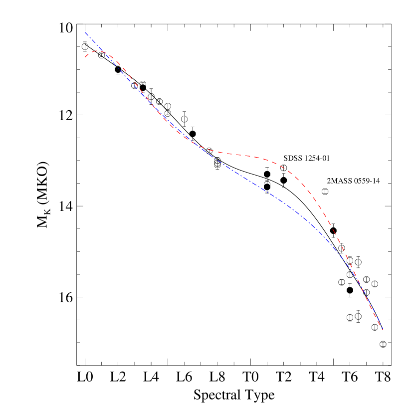
Figure 3: Absolute MKO $K$-band magnitude versus spectral type for 26 unresolved field sources (open circles) and the eight components of the binaries Kelu 1AB, Epsilon Indi Bab, SDSS 0423-0414AB and SDSS 1021-0304AB (filled circles). Photometric data are from Geballe et al. (2002); Leggett et al. (2002); Knapp et al. (2004); McCaughrean et al. (2004); Liu & Leggett (2005); and Burgasser et al. (2006a). Parallax data are from Dahn et al. (2002); Tinney, Burgasser, & Kirkpatrick (2003); and Vrba et al. (2004). A eighth-order polynomial fit to these data is indicated by the black line (see Table 3). $M_{K}$/spectral type relations from Liu et al. (2006), excluding known binaries (red dashed line) and known and possible binaries (blue dot-dashed line) are also shown.

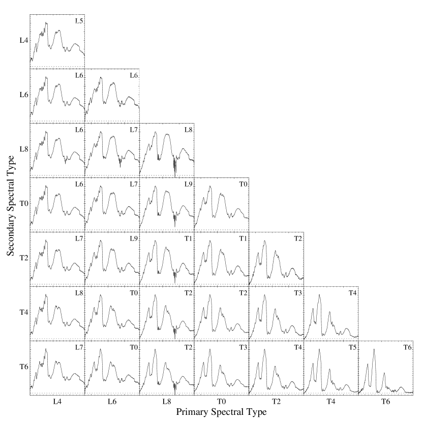
Figure 4: Hybrid binary spectra for various combinations of primary (ordinate) and secondary (abscissa) spectral type combinations. All spectra are normalized in the 1.1–1.3 $\micron$ band. Composite spectral types, based on spectral indices as described in $\S$ 3.5.2, are indicated in the upper right corner of each box.

The spectral templates were then calibrated to absolute fluxes according to an adopted absolute magnitude scale. Three MKO $M_{K}$/spectral type relations and two $M_{J}$/spectral type relations were examined. The primary relation used in the simulations was derived by fitting an eighth-order polynomial to $M_{K}$ data based on photometry (Geballe et al., 2002; Leggett et al., 2002; Knapp et al., 2004) and parallax data (Dahn et al., 2002; Tinney, Burgasser, & Kirkpatrick, 2003; Vrba et al., 2004) for 26 unresolved field L and T dwarfs with combined uncertainties $\leq$0.2 mag; and component absolute magnitudes for the binaries Epsilon Indi Bab (McCaughrean et al., 2004), Kelu 1AB (Liu & Leggett, 2005), SDSS J0423-0414AB and SDSS J1021-0304AB (Burgasser et al., 2006a). Figure 3 displays these data and the polynomial fit, which has a dispersion of 0.26 mag (coefficients are listed in Table 3). Again, the overluminous sources 2MASS 0559-1404 and SDSS 1254-0122 were excluded from the fit. The other absolute magnitude/spectral type relations were taken from Liu et al. (2006), based on fits to the absolute magnitudes of field sources excluding either known (“L06”) or known and possible binaries (“L06p”; see $\S$ 5.2). Figure 3 compares the three $M_{K}$/spectral type relations. The most significant differences between these lie in the L8 to T5 range, over which the two relations of Liu et al. (2006) differ by $\sim$1 mag. The polynomial fit derived here is intermediate between these two relations. The $M_{J}$/spectral type relations considered here are illustrated in Figure 4 of Liu et al. (2006).

Once the template spectra were scaled to their respective absolute magnitudes following standard techniques (cf. Cushing, Rayner & Vacca (2005)), composite spectra were created by adding the templates that bracketed the assigned spectral types of the binary components, weighted accordingly. Examples of composite spectra for various combinations of primary and secondary spectral types are illustrated in Figure 4.

3.5.2 Classifying the Composite Spectra

For binaries with large differences in their component spectral types, composite spectra can differ substantially in their spectral characteristics from the underlying standard sequence. Examples include the appearance of CH₄ absorption at $H$-band and not $K$-band, as observed in the L6: + T4: binary 2MASS J05185995-2828372AB (Cruz et al., 2004; Burgasser et al., 2006a, cf. Figure 4); or strong deviations in individual H₂O absorption bands. As tens to hundreds of thousands of composite spectra were generated in each simulation, an automated classification scheme was required After experimenting with various techniques, it was determined that classification by spectral indices provided the most efficient and accurate method.

For T dwarfs, classification by indices is straightforward, as Burgasser et al. (2006a) have defined five near-infrared indices (H₂O-J, CH₄-J, H₂O-H, CH₄-H and CH₄-K) which track monotonically with T spectral type. For the L dwarfs, several near-infrared indices have been defined and compared against optical types (Reid et al., 2001a; Testi et al., 2001; Geballe et al., 2002; McLean et al., 2003), the most successful of which are tied to the H₂O absorption bands. However, a robust classification scheme for L dwarfs in the near-infrared is still lacking, which can lead to problems particularly at the L/T transition (Chiu et al., 2006). I therefore examined the behavior of the Burgasser et al. (2006a) indices for both L and T dwarf spectra from the SpeX prism library, as shown in Figure 5. Following the convention of the empirical binary sample, spectral types for L0-L8 dwarfs are based on optical data while those for L9-T8 dwarfs are based on near-infrared data. There are strong correlations for three of these indices — the two H₂O indices and CH₄-K — that are roughly monotonic across full spectral type range. CH₄-J and CH₄-H are strongly correlated only in the T dwarf regime. Fourth-order polynomial fits to the indices were made where correlations were strongest, and coefficients are listed in Table 3.

Spectral types for the composite spectra were determined from these spectal index relations, as follows. First a spectral type was estimated from the H₂O-J, H₂O-H and CH₄-K indices. If these indices indicated a T spectral type, or if CH₄ absorption is present at $H$-band (indicated by CH₄-H $<$ 0.97), subtypes based on the CH₄-J and CH₄-H indices were also computed. The individual index spectral types were then averaged to derive an overall classification for the composite. Figure 4 lists the classifications derived for the binary combinations shown there.

To determine the robustness of this method, the L and T dwarf SpeX spectra used to derive the index relations were reclassified by the above technique and compared to their original classifications. Figure 6 illustrates this comparison and typical deviations. Overall, spectral types derived from the indices agree with published values to within 0.6 subtypes, although the scatter is greater amongst L0-L8 dwarfs (0.9 subtypes) than L9–T8 dwarfs (0.3 subtypes) or L8–T4 dwarfs (0.4 subtypes). These deviations likely arise from the same photospheric condensate variations that have inhibited the identification of near-infrared L dwarf spectral standards (Stephens, 2003). Nevertheless, Figure 6 indicates an overall accuracy of 0.5-1.0 subtypes can be attained for both L dwarfs and T dwarfs using a common set of spectral indices.

3.6 Constructing Magnitude-limited Samples

Once the parameters for all single and composite systems were derived, the simulated population was resampled into integer spectral type bins to derive distributions in number density and binary fraction. These distributions were normalized according to the assumed space density ($\S$ 3.2), yielding a “volume-limited” sample. The resulting number densities were then converted to surface densities for a magnitude-limited sample by computing effective volumes for each system,

$$V_{eff,i}=\frac{1}{3}10^{0.6(m_{lim}-M_{i})+3}~{}{\rm pc}^{3}$$ (1)

(Schmidt, 1968), where $m_{lim}$ is the adopted limiting magnitude and $M_{i}$ the absolute magnitude of the system (i.e., the absolute magnitude of a single source or the combined light magnitude for a binary system). For all simulations, $m_{lim}$ = 16 was adopted as a proxy. Surface densities to this magnitude limit were then computed as the sum of effective volumes over a given spectral type range,

$$\Sigma({\rm SpT)}=\sum_{i}^{i\in{\rm SpT}}2.424{\times}10^{-5}V_{eff,i}~{}{\rm deg}^{-2}$$ (2)

where the numerical factor provides units of deg^-2.

4 Results

A total of 58 separate simulations were run to sample the various input parameters listed in Table 2. From each simulation, volume-limited space densities, magnitude-limited surface densities, and binary fraction distributions (for both volume-limited and magnitude-limited cases) as a function of primary, secondary and systemic (singles plus composite binaries) spectral type were constructed. In the comparisons that follow, the baseline simulation is based on the Baraffe et al. (2003) evolutionary models, a power-law mass function with $\alpha$ = 0.5, ${\epsilon}_{b}$ = 0.1, the exponential mass ratio distribution, and the $M_{K}$/spectral type relation derived in $\S$ 3.5.1.

4.1 Number and Surface Density Distributions

While the focus of this study is the binary fraction distribution of L and T dwarfs, several clues into its origin can be gleaned from examining the number density (for the volume-limited case) and surface density (for the magnitude-limited case) distributions and their dependencies on various underlying parameters. Results from representative simulations are provided in Tables 5 and 6.

4.1.1 Distribution of Single Sources and Dependencies on the Underlying Mass Function

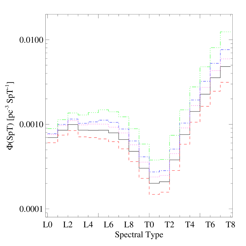
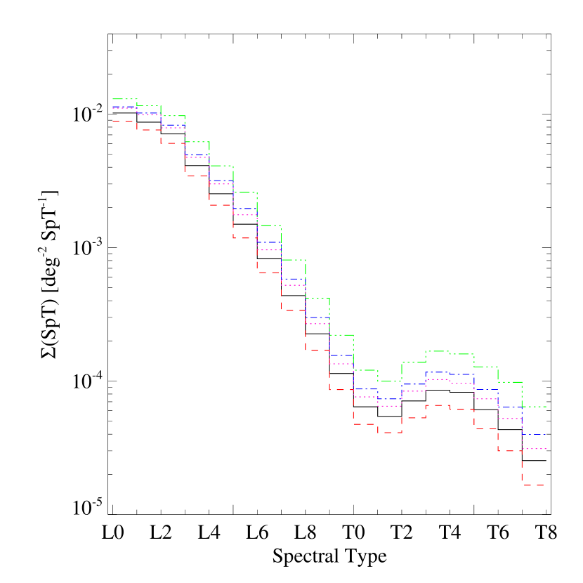
Figure 7: Number ($\Phi$(SpT); left panel) and surface density ($\Sigma$(SpT); right panel) distributions for single sources based on simulations using power-law mass functions with $\alpha$ = 0 (red dashed line), 0.5 (solid black line), 1.0 (blue dot-dashed line) and 1.5 (green triple-dot-dashed line), and the lognormal distribution of Chabrier (2002, magenta dotted line). Number densities are shown in units of pc^-3 SpT^-1 for a volume-limited sample, surface densities are shown in units of deg^-2 SpT^-1 for a magnitude-limited sample with $K\leq 16$.

Figure 7 plots the distribution of singles sources (i.e., for ${\epsilon}_{b}$ = 0) as a function of spectral type for volume-limited and magnitude-limited samples and the five mass functions examined. The overall shape of the volume-limited distributions is similar for all of the mass functions, with a plateau amongst early- and mid-type L dwarfs, followed by a decline in number density from mid-type L to a minimum around T0–T2 (a factor of 4-5 decrease); then, a rapid rise toward the latest-type T dwarfs. The shape of these distributions is similar in form to the simulated field brown dwarf luminosity functions of Burgasser (2004) and Allen et al. (2005), and arises from the combination of long-lived stellar-mass early-type L dwarfs (which accumulate over the 10 Gyr of the simulation), the rapid cooling rate of substellar-mass L dwarfs (reducing the number of late-type L dwarfs) and the slow cooling rate of late-type T dwarfs (increasing their numbers). The dip at T0–T2 is enhanced by the flattening in the $M_{bol}$/spectral type relation over this range, which spreads the luminosity function thinly at these spectral types. In addition, mass functions with $\alpha>0$ preferentially produce lower-mass brown dwarfs and hence contribute to the rise in number density amongst the lowest-luminosity brown dwarfs. Overall number densities increase for steeper power-law mass functions, as expected, ranging over 15–60% from types L0 to T8 for $\Delta\alpha$ = 0.5. The log-normal mass function produces a distribution intermediate between the $\alpha$ = 0.5 and 1.0 distributions. The number density of L0–L9 (T0–T8) dwarfs in these simulations range over 0.006–0.011 pc^-3 (0.009–0.03 pc^-3) for $\alpha$ = 0 to 1.5; i.e., there are 50–250% more T dwarfs than L dwarfs in a given volume for the mass functions examined. The number density of L/T transition objects, L8–T4, range over 0.0018–0.004 pc^-3 for $\alpha$ = 0 to 1.5, and are thus comparatively rare.

In the magnitude-limited case, the number density decline from mid-type L to early-type T combined with the decrease in absolute $K$-band brightness over this range results in a steep decline in surface densities, by a factor of $\sim$120-200 from L0 to T1 depending on the underlying MF. Surface densities then increase by $\sim$60–70% over types T1–T4, driven by both the increase in number densities and the flattening of the $M_{K}$/spectral type relation over this spectral type range. Beyond T4, surface densities again drop as the $M_{K}$/spectral type relation steepens. The intrinsic brightness of L dwarfs implies that there are 50–80 times more of these objects than T dwarfs in a given magnitude-limited sample, in stark contrast to the ratio of number densities. Again, steeper mass functions result in more L and T dwarfs, by roughly the same factor as the volume-limited case.

4.1.2 Distributions of Primaries, Secondaries and Systems

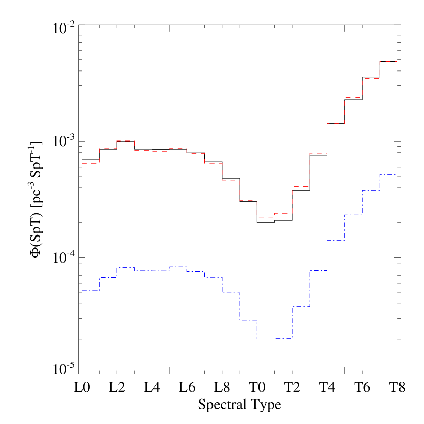
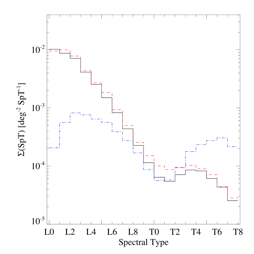
Figure 8: Number (left panel) and surface density (right panel) distributions for primaries (solid black lines), secondaries (blue dot-dashed lines) and systems (red dashed lines) for the baseline simulations. Surface densities are based on a magnitude-limited sample ($K\leq 16$).

Figure 8 compares the spectral type distributions of primaries, secondaries and systems (singles plus binaries) in both volume-limted and magnitude-limited cases. The only clear difference seen between the primary and systemic number density distributions in the volume-limited case is a 10-15% increase in the number of T0–T2 dwarf systems. This deviation increases for higher binary fractions, and while relatively small nevertheless has a significant impact on the binary fraction distribution. For the magnitude-limited distribution, the contribution of binaries in the surface densities of T0–T2 dwarfs increases substantially, by $\sim$60% for ${\epsilon}_{b}$ = 0.1, implying that 40% of these objects are binary. This is consistent with the observed binary fraction for these spectral types (Table 1). Increasing the underlying binary fraction raises the entire surface density distribution in the magnitude-limited case, as the overluminous, unresolved binaries are sampled to larger distances and greater volumes. However, the largest increase is consistently seen in the surface densities of T0–T2 dwarfs, reaching a factor of 4 increase for ${\epsilon}_{b}$ = 0.5.

The shape of the number density distribution of secondaries in Figure 8 closely follows that of the primaries and composites, but is scaled roughly by the underlying binary fraction. There is a slight increase in the relative numbers of T dwarf secondaries, an artifact of the constraint that secondaries have equal or lower masses than their primaries. Since M dwarf primaries are not modeled here, there is an artificial deficit of L dwarf secondaries. This bias is greatly enhanced in the magnitude-limited case. Interestingly, the number of T dwarf secondaries is substantially larger than the number of primaries in this case, by a factor of 3 or more for spectral types T4 and later and ${\epsilon}_{b}$ = 0.1. The vast majority of these secondaries are low mass companions to L dwarfs, as their relative infrequency (lying on the tail of the power-law mass ratio distribution) is outweighed by the much larger number of brighter L dwarf primaries in a magnitude-limited sample. A significant fraction of these systems consistent of old, low-mass stellar (L dwarf) + brown dwarf (T dwarf) pairs whose components straddle the hydrogen burning limit. These results indicate that, for a given magnitude limited sample, many more T dwarfs may be found as companions to higher mass brown dwarfs and/or stars than as isolated objects, although uncovering these companions may be nontrivial.

4.1.3 Dependencies on the Underlying Absolute Magnitude Relation

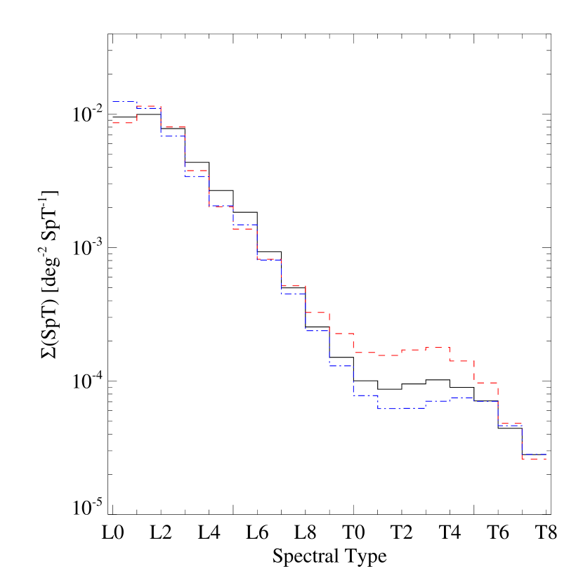
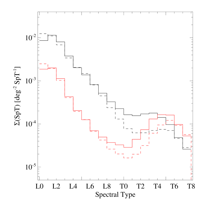
Figure 9: Surface density distributions as a function of systemic spectral type for different absolute magnitude/spectral type relations. (Left panel) $M_{K}$/spectral type relations from this study (black line; Table 3) and Liu et al. (2006), excluding known (red dashed line) and known and possible binaries (blue dot-dashed line). (Right panel) Comparison of $M_{J}$ (red lines) and $M_{K}$ (black lines) spectral type relations from Liu et al. (2006) excluding known (solid line) and known and possible binaries (dashed lines). All distributions are based on a magnitude-limited sample with a limiting magnitude of 16 in their respective bands.

The spectral type distribution of a magnitude-limited survey is naturally influenced by the underlying absolute-magnitude relation. As illustrated in Figure 9, the most significant differences found in these simulations are largely constrained to L/T transition objects, where the three absolute magnitude/spectral type relations considered here vary appreciably. Most pertinent are the differences between simulations based on the two $M_{K}$/spectral type relations of Liu et al. (2006), which differ by up to a factor of 2-5 over the L8–T5 range. This is consistent with the $\sim$1 mag difference between these relations, implying a factor of $\sim$4 increase in volume sampled. The large differences in the surface densities imply that a complete magnitude-limited sample of L/T transition objects can provide a robust constraint on the underlying absolute magnitude relation. Similar results are also found between different $M_{J}$/spectral type relations. Figure 9 also illustrates the differences between $J$-band limited and $K$-band limited samples. Surface density distributions in the former case show considerably more structure, with more pronounced local minima and maxima at types T0 and T5, respectively. This reflects the color shift between L dwarfs and T dwarfs (from red to blue $J-K$ colors), the sharper turnover in $M_{J}$/spectral type relations across the L/T transition (cf. Figure 4 in Liu et al. (2006)) and the increase in number densities beyond T0 (Figure 7).

4.1.4 Weakly Correlated Parameters

Several factors considered in the simulations contributed minimally to the overall shape of the number density and surface density distributions. These include the different minimum ages for the field population examined, spanning 0.01 to 1 Gyr, which only served to decrease the number of early-type L dwarfs by $<$15%. This is consistent with the results of Burgasser (2004), which demonstrated that only extreme modulations of the birthrate change the luminosity function of brown dwarfs appreciably. The two evolutionary models examined also produced similar spectral type distributions, with small deviations amongst early-type L dwarfs arising from different hydrogen-burning minimum masses derived by these models (0.075 M_☉ for Burrows et al. 1997 versus 0.072 M_☉ for Baraffe et al. 2003). Constant and exponential mass ratio distributions produced nearly identical spectral type distributions for ${\epsilon}_{b}$ = 0.1, although 30% differences in the surface densities of T0–T4 systems are seen for ${\epsilon}_{b}$ = 0.5. Just as an increase in the underlying binary fraction increases the total effective volume sampled for a given subclass, the exponential mass ratio distribution, which favors equal-mass/equal-brightness binaries, samples a larger effective volume than a flat mass ratio distribution. However, this effect is considerably smaller than the increase in number and surface densities (particularly amongst L/T transition objects) incurred by an increase in the underlying binary fraction. While all of these differences between the simulations are statistically significant, they are considerably smaller than current empirical uncertainties for L and T dwarf number and surface density measurements (Burgasser, 2001; Cruz et al., 2003), and can be considered negligible for the purposes of this study.

4.2 Binary Fraction Distributions

4.2.1 Reproducing the Binary Excess

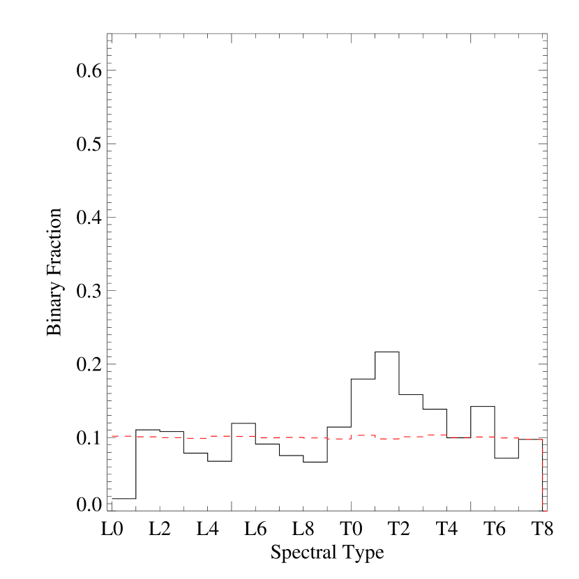
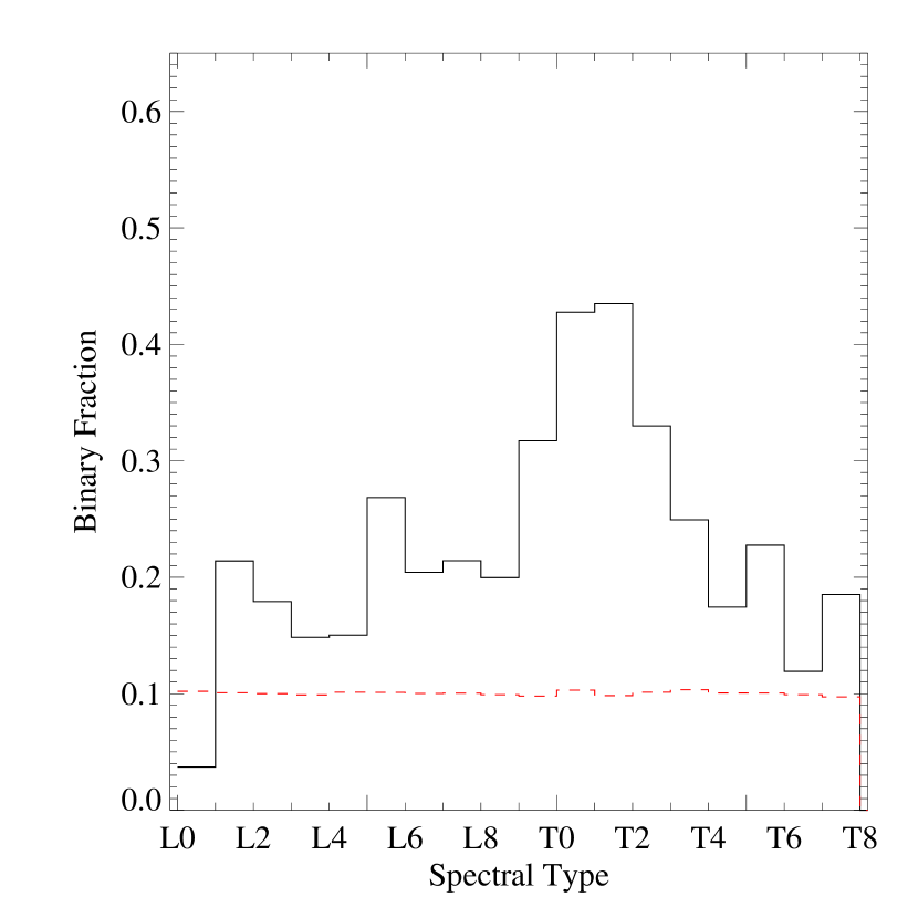
Figure 10: Binary fraction distributions for volume-limited (left) and magnitude-limited samples (right). In both panels, the binary fraction as a function of systemic spectral type is indicated in black, while the input binary fraction distribution is indicated in red (${\epsilon}_{b}$ = 0.1).

Binary fractions as a function of spectral type were computed by ratioing the number of binaries within a given systemic spectral type range to all simulated sources within that same range. Results from representative simulations for both volume-limited and magnitude-limited cases are given in Tables 7 and 8, respectively. Figure 10 displays the binary fraction distribution as a function of systemic spectral type for the baseline simulations. For both volume-limited and magnitude-limited samples, there is a considerable degree of structure in these distributions, deviating significantly from the underlying flat form. The largest jump is seen amongst T0–T2 dwarfs, over which binary fractions increase by a factor of two in the volume-limited case. The remaining low-level structure, of order 30–50%, likely arises from composite spectral classification errors or, in the case of L0–L1 dwarfs, endpoint effects. However, these are significantly smaller than the strong peak in the binary fraction distribution at types T0–T2.

In the magnitude-limited case, all binary fractions are consistently higher, a well-understood bias incurred by the larger volume sampled by overluminous, unresolved pairs. For the most part, this bias merely serves to enhance the structure seen in the volume-limited distribution and, most importantly, the fraction of binaries amongst T0–T2 dwarfs, which rises to 0.43. This result was anticipated by the increase in the surface density distribution between systems and singles as noted in $\S$ 4.1.2 (Figure 8).

That the fraction of binaries amongst T0–T2 dwarfs is higher in a volume-limited sample suggests that the intrinsic binary fraction of early-type T dwarfs is higher. However, it is important to make a distinction between the binary fraction distribution of systems and that of primaries. The latter exhibit a flat distribution in both the volume-limited and magnitude-limited cases, consistent with the assumed fixed underlying binary fraction. A more appropriate conclusion is that early-type T dwarf systems are more frequently binary, when such systems are unresolved.

4.2.2 Comparison to Empirical Data and Constraints on the Underlying Binary Fraction

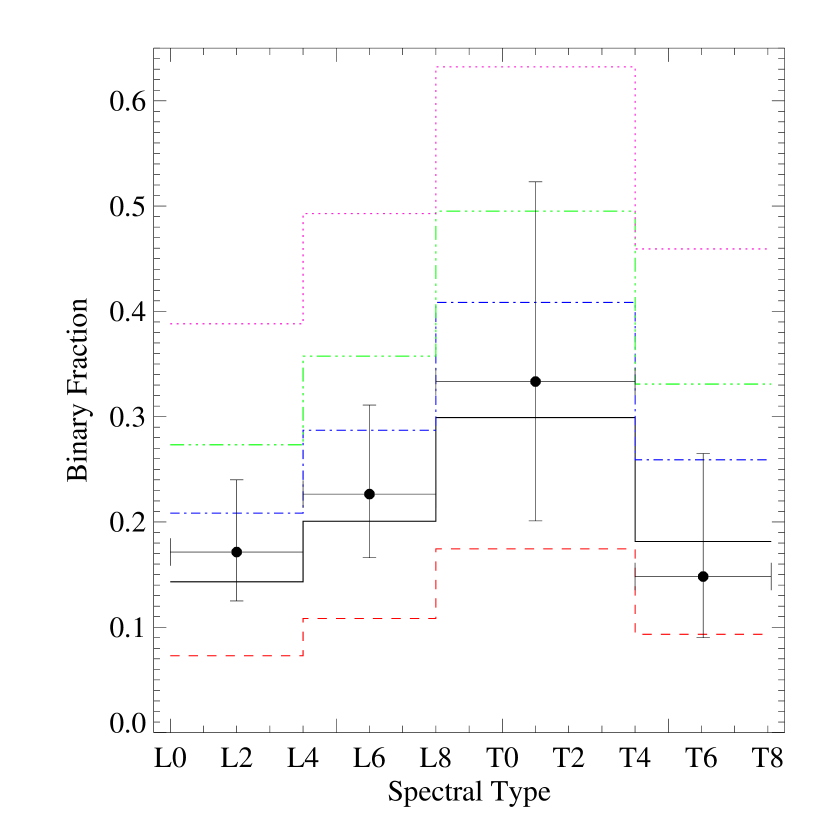
Figure 11: Binary fraction distributions for a magnitude-limited sample with ${\epsilon}_{b}$ = 0.05 (red dashed line), 0.1 (black line), 0.15 (blue dot-dashed line), 0.2 (green triple-dot dashed line) and 0.3 (magenta dotted line), resampled into spectral type bins of L0–L4, L4–L8, L8–T4, and T4–T8. Empirical measurements are indicated by solid circles with error bars, where the uncertainties correspond to the 90% confidence intervals for a binomial distribution (Burgasser et al., 2003).

Figure 11 compares the magnitude-limited binary fraction distribution as a function of systemic spectral type to the binned empirical data of Table 1. The agreement between these for the baseline parameters is quite remarkable. The steady rise in the binary fraction between early-type L dwarfs and L/T transition objects, the peak of the distribution in the latter case, and the subsequent drop in the binary fraction for the latest-type T dwarfs are all faithfully reproduced in both form and magnitude.

Figure 11 also illustrates how the binary fraction distribution varies with the assumed underlying binary fraction, ${\epsilon}_{b}$. It is seen that while increasing ${\epsilon}_{b}$ increases the scale of the distribution, it has little effect on its shape; in particular, the relative number of binaries between L/T transition objects and early-type L or later-type T dwarfs.

Comparison between these distributions and the empirical data enable a constraint on ${\epsilon}_{b}$. By linearly interpolating the distributions as a function of ${\epsilon}_{b}$ and minimizing the uncertainty-weighted deviations between the data and simulation results, a best fit ${\epsilon}_{b}^{res}$ = 0.11 was found, with ranges of 0.09–0.15 (0.08–0.17) acceptable at the 90% (95%) confidence levels. These values are fully consistent with earlier estimates of the volume-limited, resolved binary fraction of L and T dwarfs, also ranging over 0.09–0.15 (Bouy et al., 2003; Burgasser et al., 2003, 2006a; Reid et al., 2006). It is important to remember that ${\epsilon}_{b}^{res}$ is the underlying resolved binary fraction, having been constrained by observations of resolved systems. The difference between this and the intrinsic binary fraction of brown dwarfs is discussed further in $\S$ 5.2.

4.2.3 Dependencies on the Mass Ratio Distribution

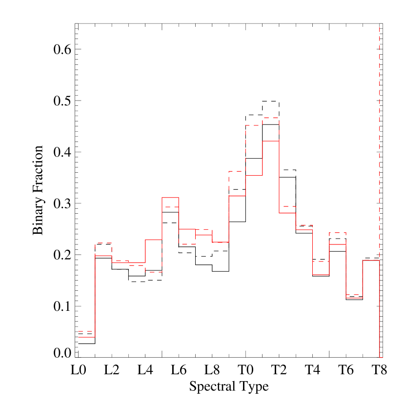
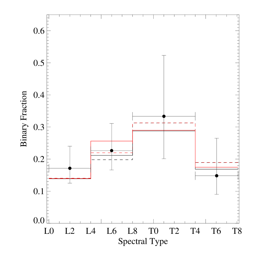
Figure 12: Binary fraction distributions for magnitude-limited samples assuming different forms of the Liu et al. (2006) $M_{K}$ (black lines) and $M_{J}$ (red lines) spectral type relations, excluding known (solid lines) or known and possible binaries (dashed lines). The left panel shows the distributions sampled by integer spectral type; the right panel shows the same distributions sampled by the spectral bins listed in Table 1. Empirical measurements are indicated in the right panel as in Figure 11.

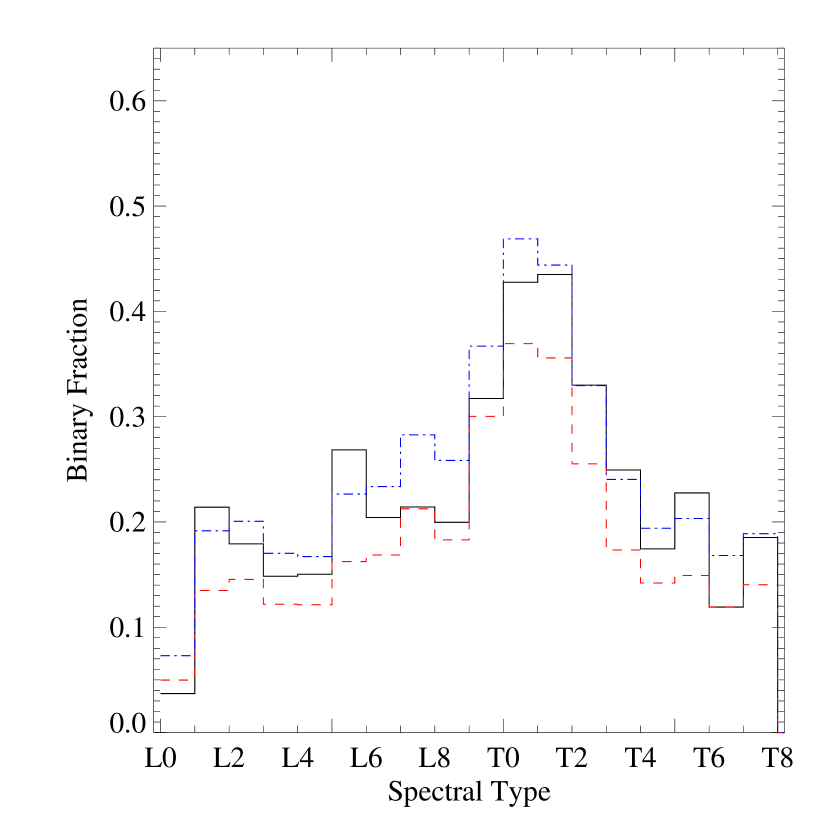
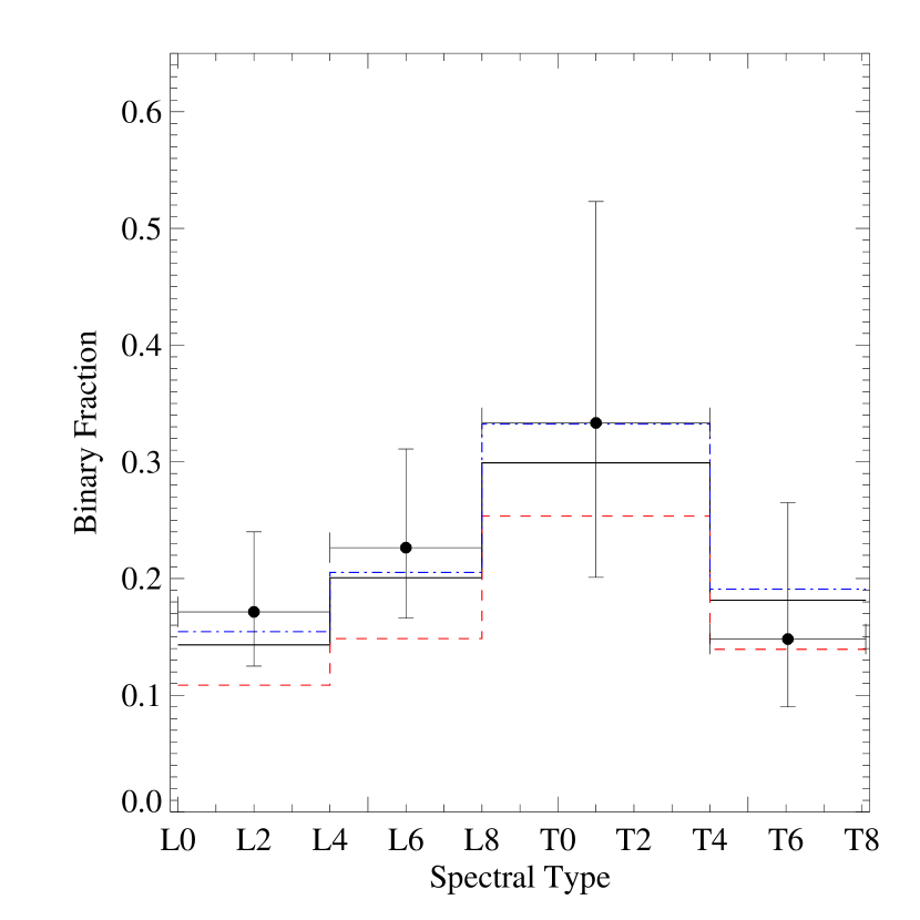
Figure 13: Binary fraction distributions for magnitude-limited samples assuming different forms of the underlying mass ratio distribution. Black lines plot distributions assuming ${\epsilon}_{b}$ = 0.1 and $P(q)\propto q^{4}$, red dashed lines plot distributions assuming ${\epsilon}_{b}$ = 0.1 and $P(q)\propto$ constant, and blue dot-dashed lines plot distributions assuming ${\epsilon}_{b}$ = 0.14 and $P(q)\propto 1$. The left panel shows the binary fraction distributions sampled by integer spectral type; the right panel shows the same distributions sampled by the spectral bins listed in Table 1. Empirical measurements are indicated in the right panel as in Figure 11.

A somewhat larger modulation of the apparent binary fraction distribution is seen when different mass ratio distributions are considered, as illustrated in Figure 13. A flat mass ratio distribution results in a 20-30% decline in the binary fraction distribution across the full spectral type range, in both the binned and unbinned cases. Again, this decline is consistent with the reduction in effective volume sampled by the reduced fraction of equal-mass/equal-brightness systems for a magnitude-limited survey. Figure 12 illustrates that a simulation using a flat mass ratio distribution and ${\epsilon}_{b}$ = 0.14 produces a binary fraction distribution that differs by less than 10% from the baseline simulation. Indeed, the empirical data constrain a best fit ${\epsilon}_{b}^{res}$ = 0.14 and acceptable ranges of 0.12–0.19 (0.11–0.21) at the 90% (95%) confidence limits in the case of a flat mass ratio distribution, somewhat higher than that derived using an exponential distribution. This degeneracy between the mass ratio distribution and the underlying binary fraction implies that the former cannot be robustly constrained by the binary fraction distribution without an independent determination of ${\epsilon}_{b}$.

4.2.4 Dependencies on the Absolute Magnitude/Spectral Type Relation

Figure 12 illustrates how the binary fraction distribution varies for different underlying absolute magnitude distributions. Despite the substantial effect that the absolute magnitude relation has on the surface density distribution of L8–T5 dwarfs (Figure 9), the impact on the binary fraction distribution is considerably smaller. Between the L06 and L06p $M_{K}$/spectral type relations, binary fraction distributions differ by less than 20% for individual subtypes, and by less than 10% when the spectral types are binned according to the empirical data. There is a comparably small difference between binary fraction distributions generated by the $M_{J}$/spectral type relations of Liu et al. (2006), and also between $J$- and $K$-band magnitude-limited samples. These comparisons indicate that the binary fraction distribution, and more importantly the binary excess at the L/T transition, are relatively insensitive to the details of how a magnitude-limited sample is constructed. This justifies the incorporation of several high-resolution imaging samples into a single magnitude-limited probe of the binary fraction distribution.

A more important conclusion to draw from these comparisons, however, is that the observed binary excess does not appear to be an artifact of magnitude-limited imaging samples, since the parameters that most influence the surface densities of L and T dwarfs (the absolute magnitude scale and limiting filter band) have little bearing on the binary fraction distribution. Indeed, as already pointed out in $\S$ 4.2.1, a magnitude-limited sample simply amplifies the excess present in the underlying population.

4.2.5 Weakly Correlated Parameters

As with the number and surface density distributions, several of the parameters explored in these simulations had minimal influence on the binary fraction distribution. Neither the form of the mass function, choice of evolutionary model or minimum age of the population had more than a 5% effect on the structure or magnitude of the distribution. Out of all of the parameters varied, only ${\epsilon}_{b}$ significantly influences the binary fraction distribution and only by scaling the entire distribution up or down. The structure of the distribution — i.e., the excess of binaries amongst L/T transition objects — must arise from some other aspect of the simulation. As discussed below, it appears that the luminosity scale is exclusively responsible for this excess.

5 Discussion

5.1 On the Origin of the L/T Transition Binary Excess

The simulations presented here reproduce remarkably the relatively high binary fraction of L/T transition brown dwarfs. Yet how does this binary excess arise? Both Burgasser et al. (2006a) and Liu et al. (2006) proposed that the similarity of the composite spectra of L + T dwarf binaries to early-type T dwarf spectral morphologies, and the rapid evolution of single brown dwarfs through the L/T transition, may be the underlying causes. A detailed examination of the simulations presented here support these hypotheses.

First, the composition of L/T transition binaries in the simulations is quite distinct as compared to other spectral subclasses, as illustrated in Figure 14. Most binaries have composite types similar to their primaries, reflecting both the preference for equal-mass/equal-luminosity systems in the exponential mass ratio distribution and the dominance of the primary in the combined light spectrum of systems with low-mass companions. Yet binaries classified as L9–T3 dwarfs consistently have earlier-type primaries, up to $\sim$0.6 subclasses on average, while 15-20% of T0–T2 systems have primaries at least one subclass earlier. This is consistent with studies of known L/T transition binaries, 70% of which have been shown or inferred to be L dwarf plus T dwarf pairs (Burgasser et al., 2006a). Such pairs readily mimic the spectral appearance of an early-type T dwarf. The flattening of the absolute magnitude scale across the L/T transition allows the T dwarf secondaries of these systems to contribute significantly to the overall spectral flux at near infrared wavelengths. Thus, a wide variety of component combinations result in a composite spectral energy distribution similar to an early-type T dwarf (cf. Figure 4).

Second, a rapid evolution of brown dwarfs across the L/T transition can be deduced from the flattening of the luminosity scale over this range. Based on the evolutionary models of Baraffe et al. (2003) and the $M_{bol}$/spectral type relation shown in Figure 1, a 0.05 M_☉ (0.03 M_☉) brown dwarf dims from type L8 to type T3 in $\sim$600 Myr ($\sim$100 Myr), a period spanning 30% (20%) of its lifetime at that stage. In comparison, a brown dwarf of similar mass spends 2-3 times longer cooling from L0 to L8, and a full 7 Gyr (3 Gyr) cooling thereafter to the end of the T spectral class. Since single brown dwarfs spend relatively little time at the L/T transition, they are much rarer than earlier-type and later-type brown dwarfs in a given volume (Figure 7). Yet, combinations of these other spectral types, even for small binary fractions, can be comparable in number to single L/T transition objects, resulting in the perceived binary excess.

These two explanations for the high rate of binaries amongst L/T transition objects are in fact related to a single underlying cause: the flattening of the luminosity scale. The small decline in $M_{bol}$ across the L/T transition directly translates into small changes in the absolute magnitude scale over this range, and is the root cause of the rarity of single L/T transition objects. Consider then the reverse argument: The observed excess of binaries at the L/T transition is further evidence of a flattening in the luminosity scale. Indeed, the agreement between the shape of the simulated binary fraction distribution and empirical data, which is largely independent of all other parameters besides the $M_{bol}$/spectral type relation, suggests that the luminosity scale of brown dwarfs across the L/T transition is indeed quite flat, and that brown dwarfs must traverse this transition over a relatively short period. This lends support to suggestions that the complete removal of photospheric condensate dust between late-type L and mid-type T, which appears to be largely responsible for the changes in spectral morphology across this transition, is relatively rapid and may require dynamic, nonequilibrium atmospheric processes.

5.2 Absolute Magnitudes of Field L/T Dwarfs and the Intrinsic Brown Dwarf Binary Fraction

In $\S$ 4.2.2, a constraint on the underlying resolved binary fraction, ${\epsilon}_{b}^{res}$, was made by comparing simulated binary fraction distributions to high-resolution imaging results. However, imaging cannot identify binaries that have very small separations or systems observed when the components are aligned along the line of sight (e.g., Kelu 1AB; Martín, Brandner & Basri (1999); Liu & Leggett (2005); Gelino, Kulkarni & Stephens (2006)). The existence of very tight brown dwarf binaries in the field is likely, as the separation distribution of resolved systems peaks at or near the resolution limit of current imaging surveys (Bouy et al., 2003; Gizis et al., 2003; Burgasser et al., 2006a, b). Maxted & Jeffries (2005), analyzing the results of the first searches for spectroscopic brown dwarf binaries (Basri & Martín, 1999a; Guenter & Wuchterl, 2003; Kenyon et al., 2005; Joergens, 2006), have suggested that the true binary fraction of brown dwarfs may be as high as 0.45 when selection effects are considered. Similarly, Pinfield et al. (2003) and Chapelle et al. (2005) have inferred binary fractions of 0.3–0.5 for very low mass stars and brown dwarfs in two young open clusters based on the identification of overluminous sources in the color-magnitude diagram.

For field brown dwarfs, particularly L/T transition objects, the identification of overluminous, unresolved binaries is made difficult by uncertainties in the absolute magnitude relation, as well as intrinsic scatter arising from age, surface gravity and radius differences. Nevertheless, Liu et al. (2006) hypothesized that a substantial fraction of L7–T5 dwarfs with parallax distance measurements — 10 of 15 sources (0.66${}^{+0.12}_{-0.17}$%) — are either resolved or unresolved binaries, due to their outlying position on the T_eff/spectral type relation of Golimowski et al. (2004). Taking this suggestion at face value, and assuming that the current parallax sample is essentially magnitude-limited (i.e., ignoring additional selection effects), the fraction of known and possible binaries over this spectral type range implies ${\epsilon}_{b}$ = 0.38, with an acceptable range of 0.24–0.53 (0.21–0.59) at the 90% (95%) confidence level, assuming $P(q)\propto q^{4}$. This is substantially higher than the fraction inferred from high-resolution imaging surveys, and suggests that up to twice as many brown dwarf binaries remain unresolved in these surveys. Indeed, since counting overluminous sources includes only those binaries with similar-mass companions, the intrinsic binary fraction may be higher still. This result is seemingly consistent with the high brown dwarf binary fraction proposed by Maxted & Jeffries (2005).

Care must be taken in interpreting this value since the number of L7–T5 dwarfs with parallax measurements is small, uncertainties in several of the parallax measurements large, the underlying absolute magnitude distribution poorly constrained and hence the identification of overluminous sources highly uncertain. However, if the absolute magnitude scale is relatively flat across the L/T transition, and the apparent fraction of binaries high, a measure of the fraction of overluminous sources in this spectral type regime may provide a more robust constraint on the true binary fraction of all brown dwarfs than high-resolution imaging surveys.

6 Summary

The primary results of this study are as follows:

• The binary fraction excess observed amongst L/T transition objects has been successfully reproduced by mass function simulations incorporating the construction and classification of unresolved binary systems. It is found that this excess arises largely from a flattening in the $M_{bol}$/spectral type relation, which significantly reduces the number of single L/T transition objects in a given volume while also causing L dwarf + T dwarf pairs to mimic the spectral properties of early-type T dwarfs. While the binary excess is particularly pronounced in magnitude-limited samples (hence its detection in current high resolution imaging studies), it is not caused by selection biases, but is instead intrinsic to any sample of unresolved brown dwarf systems.

• The shape of the binary fraction distribution depends weakly on the underlying absolute magnitude/spectral type relation, mass function and minimum age of the field population (up to 1 Gyr). The underlying binary fraction, ${\epsilon}_{b}$ produces the greatest effect, scaling the distribution but not significantly affecting its shape. There is a slight degeneracy between the influence of ${\epsilon}_{b}$ and the mass ratio distribution on the scale of the binary fraction distribution for a magnitude-limited sample.

• The surface density of L/T transition objects in a magnitude-limited sample is highly sensitive to the underlying absolute magnitude/spectral type relation. Number and surface densities also scale with the underlying mass function, but are largely insensitive to the minimum age of the field population or the mass ratio distribution of brown dwarf binaries.

• Empirical results constrain the underlying resolved binary fraction to 11${}_{-3}^{+6}$% (90% confidence interval), consistent with prior estimates. The true binary fraction, which includes sources unresolved in imaging studies, may be as high as 40% based on the fraction of apparently overluminous L7–T5 dwarfs as proposed by Liu et al. (2006). However, this result requires a more robust assessment of the absolute magnitude scale, and understanding a selection effects in the current parallax sample, and more (and improved) parallax measurements of L/T transition objects.

The simulations presented here provide new insight into the relationship between the fundamental properties of brown dwarfs (luminosities, mass function, intrinsic multiplicity) and the observed density, spectroscopic properties and multiplicity of L/T transition dwarfs. What they do not reveal is the physical mechanism that drives this transition. The dramatic change in spectral properties over a short evolutionary period is strong evidence that nonequilibrium dispersion of photospheric condensates must play an important, if not predominant, role. As new theoretical models address dynamical atmospheric effects that may be involved in condensate cloud evolution, continued empirical characterization of these sources — including improved multiplicity statistics through high-resolution imaging, spectroscopic monitoring, and parallax measurements — should be a priority. Fortunately, the apparently high binary fraction of L/T transition objects implies that this remarkable evolutionary phase of brown dwarfs can be studied quite thoroughly, through resolved photometric and spectroscopic studies and long-term astrometric monitoring to measure component masses. These enigmatic systems may ultimately provide the most stringent empirical constraints on the properties of brown dwarfs in general.

Table 1: Empirical Binary Fraction Data

SpT	# Total	# Binary	${\epsilon}_{b}^{obs}$	90% CI	95% CI
L0–L0.5	15	4	0.27	0.16–0.44	0.13–0.48
L1–L1.5	20	2	0.10	0.05–0.23	0.04–0.27
L2–L2.5	22	3	0.14	0.08–0.27	0.06–0.30
L3–L3.5	13	3	0.23	0.13–0.42	0.11–0.47
L4–L4.5	18	2	0.11	0.06–0.26	0.05–0.30
L5–L5.5	17	3	0.18	0.10–0.33	0.08–0.38
L6–L6.5	10	3	0.30	0.17–0.51	0.14–0.56
L7–L7.5	8	4	0.50	0.30–0.70	0.25–0.75
L8–L8.5	3	0	0.00	$<$0.44	$<$0.53
L9–L9.5	1	0	0.00	$<$0.68	$<$0.78
T0–T0.5	2	2	1.00	$>$0.47	$>$0.37
T1–T1.5	3	1	0.33	0.14–0.68	0.10–0.75
T2–T2.5	1	0	0.00	$<$0.68	$<$0.78
T3–T3.5	2	1	0.50	0.20–0.80	0.14–0.86
T4–T4.5	4	1	0.25	0.11–0.58	0.08–0.66
T5–T5.5	8	1	0.13	0.06–0.37	0.04–0.43
T6–T6.5	8	1	0.13	0.06–0.37	0.04–0.43
T7–T7.5	6	1	0.17	0.08–0.45	0.05–0.52
T8–T8.5	1	0	0.00	$<$0.68	$<$0.78
L0–L3.5	70	12	0.17	0.13–0.24	0.11–0.26
L4–L7.5	53	12	0.23	0.17–0.31	0.15–0.34
L8–T3.5	12	4	0.33	0.20–0.52	0.17–0.57
T4–T8	27	4	0.15	0.09–0.27	0.07–0.30

Note. — Data compiled from high resolution imaging surveys by Martín, Brandner & Basri (1999); Reid et al. (2001b, 2006); Bouy et al. (2003); Burgasser et al. (2003, 2006a); Close et al. (2003); Gizis et al. (2003); Liu & Leggett (2005); and Gelino, Kulkarni & Stephens (2006).

Table 2: Input Parameters for Monte Carlo Simulations.

Parameter	Form and Details
Mass Function	$\Psi({\rm M})\propto{\rm M}^{-{\alpha}}$, with $\alpha$ = 0.0, 0.5, 1.0, 1.5
	$\Psi({\rm M})\propto{\rm e}^{-\frac{({\rm\log{M}}-{\rm\log{M_{c}}})^{2}}{2{\sigma}^{2}}}$, with ${\rm M_{c}}=0.1{\rm M}_{\sun},\sigma=0.627$
Age Distribution	$P(t)\propto$ constant, with $t\in\{T_{0},10~{}{\rm Gyr}\}$, $T_{0}$ = 0.1, 0.5, 1.0 Gyr
Evolutionary Model	Baraffe et al. (2003); Burrows et al. (2001)
${\epsilon}_{b}$	0, 0.05, 0.1, 0.14, 0.15, 0.2, 0.25, 0.3, 0.35, 0.4, 0.45, 0.5, 0.55, 0.6, 0.7
Mass Ratio Distribution	$P(q)\propto q^{\Gamma}$, with $\Gamma$ = 4
	$P(q)\propto$ constant
$M_{bol}$/SpT Relation	This paper (see Table 3)
$M_{K}$/SpT Relation	This paper (see Table 3)
	Liu et al. (2006)
$M_{J}$/SpT Relation	Liu et al. (2006)

Table 3: Polynomial Fits to Spectral Type Relations

		Coefficients
Parameter	Range	$c_{0}$	$c_{1}$	$c_{2}$	$c_{3}$	$c_{4}$	$c_{5}$	$c_{6}$	$c_{7}$	$c_{8}$	$\sigma$
$M_{bol}$(SpT)	L0–T8	1.374e1	1.903e-1	1.731e-2	7.400e-3	-1.751e-3	1.142e-4	-2.322e-6	$\cdots$	$\cdots$	0.22 mag
$M_{K}$(SpT)	L0–T8	1.045e1	2.322e-1	5.129e-2	-4.024e-2	1.414e-2	-2.271e-3	1.807e-4	-6.985e-6	1.051e-7	0.26 mag
SpT(H2O-J)	L0–T8	1.949e1	-3.919e1	1.312e2	-2.156e2	1.038e2	$\cdots$	$\cdots$	$\cdots$	$\cdots$	0.8 SpT
SpT(CH4-J)	T0–T8	2.098e1	-1.978e1	2.527e1	-3.221e1	9.087e-1	$\cdots$	$\cdots$	$\cdots$	$\cdots$	0.7 SpT
SpT(H2O-H)	L0–T8	2.708e1	-8.450e1	2.424e2	-3.381e2	1.491e2	$\cdots$	$\cdots$	$\cdots$	$\cdots$	1.0 SpT
SpT(CH4-H)	T1–T8	2.013e1	-2.291e1	4.361e1	-5.068e1	2.084e1	$\cdots$	$\cdots$	$\cdots$	$\cdots$	0.3 SpT
SpT(CH4-K)	L0–T7	1.885e1	-2.246e1	2.534e1	-4.734e0	-1.259e1	$\cdots$	$\cdots$	$\cdots$	$\cdots$	1.1 SpT

Note. — Polynomials relations are defined as $f(x)=\sum_{i}{c_{i}x^{i}}$. SpT is the numerical spectral type defined as SpT(L0) = 0, SpT(L5) = 5, SpT(T0) = 10, etc.

Table 4: Spectral Templates

	Spectral Type		2MASS Photometry
Name	Opt	NIR	$J$	$J-K_{s}$	$\pi$	Ref
			(mag)	(mag)	(marcs)
(1)	(2)	(3)	(4)	(5)	(6)	(7)
2MASS J03454316+2540233	L0	L1$\pm$1	14.00$\pm$0.03	1.33$\pm$0.04	37.1$\pm$0.5	1,2,3
2MASS J14392836+1929149	L1	$\cdots$	12.76$\pm$0.02	1.21$\pm$0.03	69.6$\pm$0.5	2,4
SSSPM J0829-1309	L2	$\cdots$	12.80$\pm$0.03	1.51$\pm$0.04	$\cdots$	5,6
2MASS J15065441+1321060	L3	$\cdots$	13.37$\pm$0.02	1.62$\pm$0.03	$\cdots$	7
2MASS J11040127+1959217	L4	$\cdots$	14.38$\pm$0.03	1.43$\pm$0.04	$\cdots$	8
GJ 1001BC	L5	L4.5	13.11$\pm$0.02	1.71$\pm$0.04	77$\pm$4	3,9,10,11
2MASS J04390101-2353083	L6	$\cdots$	14.41$\pm$0.03	1.59$\pm$0.04	$\cdots$	8
2MASS J09153413+0422045	L7	$\cdots$	14.55$\pm$0.03	1.54$\pm$0.05	$\cdots$	12
DENIS J025503.3$-$470049	L8	$\cdots$	13.25$\pm$0.03	1.69$\pm$0.04	$\cdots$	13,14
2MASS J03105986+1648155	L8	L9	16.03$\pm$0.08	1.71$\pm$0.11	$\cdots$	10,15
SDSS J042348.57$-$041403.5	L7.5	T0	14.47$\pm$0.03	1.54$\pm$0.04	65.9$\pm$1.7	16,17
SDSS J015141.69+124429.6	$\cdots$	T1	16.57$\pm$0.13	1.38$\pm$0.23	47$\pm$3	15,16
SDSS J125453.90$-$012247.4	T2	T2	14.89$\pm$0.04	1.05$\pm$0.06	73.2$\pm$1.9	16,17,18
2MASS J12095613$-$1004008	$\cdots$	T3	15.91$\pm$0.07	0.85$\pm$0.16	$\cdots$	19
2MASS J22541892+3123498	$\cdots$	T4	15.26$\pm$0.05	0.36$\pm$0.15	$\cdots$	20
2MASS J15031961+2525196	$\cdots$	T5	13.94$\pm$0.02	-0.03$\pm$0.06	$\cdots$	21
SDSS J162414.37+002915.6	$\cdots$	T6	15.49$\pm$0.05	$<$-0.02	90.9$\pm$1.2	22,23
2MASS J07271824+1710012	T8	T7	15.60$\pm$0.06	0.04$\pm$0.20	110$\pm$2	17,20
2MASS J04151954$-$0935066	T8	T8	15.70$\pm$0.06	0.27$\pm$0.21	174$\pm$3	17,20

References. — (1) Kirkpatrick, Beichman, & Skrutskie (1997); (2) Dahn et al. (2002); (3) Knapp et al. (2004); (4) Kirkpatrick et al. (1999); (5) Scholz & Meusinger (2002); (6) Lodieu et al. (2005); (7) Gizis et al. (2000); (8) Cruz et al. (2003); (9) Goldman et al. (1999); (10) Kirkpatrick et al. (2000); (11) Henry et al. (2006); (12) I. N. Reid et al., in preparation; (13) Martín et al. (1999); (14) J. D. Kirkpatrick et al., in preparation; (15) Geballe et al. (2002); (16) Leggett et al. (2000); (17) Vrba et al. (2004); (18) Burgasser et al. (2003a); (19) Burgasser et al. (2004); (20) Burgasser et al. (2002); (21) Burgasser et al. (2003b); (22) Strauss et al. (1999); (23) Tinney, Burgasser, & Kirkpatrick (2003)

Table 5: Number Densities as a Function of Systemic Spectral Type

	$\Psi$(M) $\propto$	M0.0	M-0.5	M-1.0	M-1.5	lognormal	M-0.5	M-0.5
	$P(q)\propto$	$q^{4}$	$q^{4}$	$q^{4}$	$q^{4}$	$q^{4}$	$q^{4}$	$q^{4}$
	${\epsilon}_{b}$ =	0.1	0.1	0.1	0.1	0.1	0.3	0.5
L0–L1		0.555	0.637	0.712	0.812	0.692	0.503	0.396
L1–L2		0.755	0.861	1.01	1.16	0.973	0.869	0.905
L2–L3		0.848	1.00	1.16	1.37	1.12	1.01	1.01
L3–L4		0.693	0.834	1.01	1.25	0.962	0.787	0.756
L4–L5		0.672	0.819	1.03	1.33	0.964	0.767	0.707
L5–L6		0.688	0.869	1.14	1.52	1.03	0.911	0.945
L6–L7		0.618	0.785	1.04	1.39	0.914	0.764	0.746
L7–L8		0.502	0.644	0.858	1.18	0.772	0.614	0.579
L8–L9		0.351	0.462	0.607	0.856	0.555	0.428	0.393
L9–T0		0.237	0.308	0.421	0.597	0.366	0.328	0.342
T0–T1		0.165	0.220	0.294	0.412	0.261	0.251	0.297
T1–T2		0.181	0.241	0.326	0.442	0.284	0.300	0.362
T2–T3		0.304	0.406	0.549	0.780	0.475	0.452	0.503
T3–T4		0.605	0.788	1.08	1.54	0.949	0.845	0.931
T4–T5		1.06	1.42	1.94	2.76	1.66	1.40	1.41
T5–T6		1.71	2.38	3.40	5.06	2.88	2.60	2.83
T6–T7		2.39	3.45	5.09	7.79	4.18	3.23	3.01
T7–T8		3.14	4.82	7.63	12.4	5.94	4.82	4.86

Note. — Number densities in units of 10^-3 pc^-3 SpT^-1. Results listed here are based on simulations using the evolutionary models of Baraffe et al. (2003), a flat age distribution spanning 0.01–10 Gyr, the $M_{K}$/spectral type relation defined in this study ($\S$ 3.5.1), and parameters as specified in the header. Values are normalized to a number density of 0.0037 pc^-3 over the mass range of 0.09–0.1 M_☉, derived from the low-mass stellar mass function of Reid et al. (1999).

Table 6: Surface Densities for a Magnitude-Limited Sample as a Function of Systemic Spectral Type

	$\Psi$(M) $\propto$	M0.0	M-0.5	M-1.0	M-1.5	lognormal	M-0.5	M-0.5	M-0.5	M-0.5	M-0.5	M-0.5	M-0.5
	$M$(SpT):	TP-$K$	TP-$K$	TP-$K$	TP-$K$	TP-$K$	L06-$K$	L06p-$K$	L06-$J$	L06p-$J$	TP-$K$	TP-$K$	TP-$K$
SpT	$P(q)\propto$	$q^{4}$	$q^{4}$	$q^{4}$	$q^{4}$	$q^{4}$	$q^{4}$	$q^{4}$	$q^{4}$	$q^{4}$	1	$q^{4}$	$q^{4}$
	${\epsilon}_{b}$ =	0.1	0.1	0.1	0.1	0.1	0.1	0.1	0.1	0.1	0.1	0.3	0.5
L0–L1		8.24	9.52	10.6	12.1	10.3	8.62	12.4	1.87	2.49	9.56	7.92	6.69
L1–L2		8.68	9.96	11.6	13.5	11.2	11.5	11.0	2.00	1.94	8.96	12.2	15.0
L2–L3		6.58	7.80	8.99	10.7	8.70	8.02	6.85	1.13	1.02	7.41	9.02	10.4
L3–L4		3.63	4.36	5.28	6.46	5.02	3.77	3.41	0.430	0.408	4.27	4.76	5.33
L4–L5		2.21	2.68	3.37	4.30	3.13	2.02	2.06	0.205	0.195	2.63	3.00	3.29
L5–L6		1.47	1.84	2.40	3.19	2.19	1.38	1.48	0.125	0.126	1.62	2.56	3.28
L6–L7		0.736	0.932	1.22	1.63	1.08	0.818	0.806	0.0697	0.0678	0.885	1.14	1.34
L7–L8		0.398	0.500	0.663	0.894	0.600	0.518	0.449	0.0497	0.0424	0.494	0.639	0.761
L8–L9		0.194	0.254	0.325	0.464	0.305	0.327	0.239	0.0371	0.0261	0.245	0.316	0.358
L9–T0		0.119	0.151	0.205	0.285	0.182	0.227	0.130	0.0328	0.0201	0.147	0.242	0.320
T0–T1		0.0761	0.100	0.131	0.186	0.118	0.164	0.0777	0.0287	0.0163	0.0882	0.171	0.242
T1–T2		0.0656	0.0869	0.117	0.160	0.102	0.156	0.0623	0.0441	0.0199	0.0735	0.150	0.214
T2–T3		0.0712	0.0952	0.129	0.179	0.110	0.171	0.0624	0.0738	0.0316	0.0857	0.143	0.190
T3–T4		0.0781	0.102	0.138	0.199	0.123	0.179	0.0706	0.131	0.0611	0.0935	0.134	0.171
T4–T5		0.0670	0.0897	0.122	0.173	0.104	0.142	0.0749	0.164	0.0948	0.0855	0.102	0.117
T5–T6		0.0510	0.0711	0.101	0.151	0.0859	0.0968	0.0705	0.161	0.121	0.0644	0.0910	0.111
T6–T7		0.0307	0.0443	0.0652	0.0996	0.0536	0.0483	0.0463	0.0975	0.0926	0.0441	0.0462	0.0481
T7–T8		0.0184	0.0281	0.0442	0.0713	0.0346	0.0260	0.0282	0.0527	0.0565	0.0265	0.0337	0.0397

Note. — Surface densities in 10^-3 deg^-2 SpT^-1. Results listed here are based on simulations using the evolutionary models of Baraffe et al. (2003), a flat age distribution spanning 0.01–10 Gyr, and parameters as specified in the header. Values are normalized to a number density of 0.0037 pc^-3 over the mass range of 0.09–0.1 M_☉, derived from the low-mass stellar mass function of Reid et al. (1999); and assume a limiting magnitude of 16 in the appropriate photometric band.

Table 7: Binary Fraction as a Function of Systemic Spectral Type: Volume-Limited

	$\Psi$(M) $\propto$	M-0.5	M-0.5	M-0.5	M-0.5	M-0.5	M-0.5	M-0.5	M-0.5	M-0.5	M-0.5
	$M$(SpT):	TP-$K$	TP-$K$	TP-$K$	TP-$K$	TP-$K$	L06-$K$	L06p-$K$	L06-$J$	L06p-$J$	TP-$K$
SpT	$P(q)\propto$	$q^{4}$	$q^{4}$	$q^{4}$	$q^{4}$	$q^{4}$	$q^{4}$	$q^{4}$	$q^{4}$	$q^{4}$	1
	${\epsilon}_{b}$ =	0.1	0.2	0.3	0.4	0.5	0.1	0.1	0.1	0.1	0.1
L0–L1		0.0168	0.0344	0.0635	0.0888	0.127	0.0122	0.0239	0.0178	0.0272	0.0455
L1–L2		0.111	0.218	0.318	0.424	0.526	0.109	0.116	0.113	0.117	0.0967
L2–L3		0.108	0.215	0.311	0.408	0.522	0.105	0.101	0.104	0.104	0.109
L3–L4		0.0788	0.162	0.247	0.333	0.435	0.0758	0.0726	0.0759	0.0780	0.0857
L4–L5		0.0678	0.137	0.219	0.304	0.391	0.0627	0.0648	0.0598	0.0574	0.0782
L5–L6		0.119	0.229	0.339	0.446	0.547	0.110	0.114	0.106	0.112	0.0910
L6–L7		0.0911	0.178	0.275	0.373	0.467	0.0813	0.0919	0.0719	0.0763	0.0932
L7–L8		0.0755	0.154	0.245	0.331	0.422	0.0667	0.0799	0.0647	0.0717	0.100
L8–L9		0.0666	0.146	0.226	0.309	0.391	0.0627	0.0775	0.0649	0.0653	0.0873
L9–T0		0.114	0.228	0.357	0.455	0.563	0.115	0.123	0.107	0.119	0.128
T0–T1		0.180	0.326	0.459	0.573	0.651	0.204	0.176	0.184	0.192	0.168
T1–T2		0.217	0.393	0.521	0.643	0.720	0.272	0.208	0.281	0.249	0.186
T2–T3		0.159	0.294	0.416	0.521	0.621	0.187	0.141	0.200	0.162	0.138
T3–T4		0.139	0.255	0.379	0.489	0.587	0.141	0.125	0.147	0.133	0.113
T4–T5		0.0997	0.196	0.297	0.398	0.497	0.0983	0.106	0.0955	0.101	0.104
T5–T6		0.142	0.273	0.394	0.502	0.597	0.141	0.141	0.141	0.142	0.112
T6–T7		0.0718	0.147	0.228	0.316	0.409	0.0720	0.0719	0.0727	0.0727	0.0931
T7–T8		0.0975	0.201	0.298	0.399	0.501	0.0995	0.102	0.101	0.101	0.101

Note. — Results based on simulations using the evolutionary models of Baraffe et al. (2003), a flat age distribution spanning 0.01–10 Gyr, and parameters as indicated in the header.

Table 8: Binary Fraction as a Function of Systemic Spectral Type: Magnitude-Limited

	$\Psi$(M) $\propto$	M-0.5	M-0.5	M-0.5	M-0.5	M-0.5	M-0.5	M-0.5	M-0.5	M-0.5	M-0.5
	$M$(SpT):	TP-$K$	TP-$K$	TP-$K$	TP-$K$	TP-$K$	L06-$K$	L06p-$K$	L06-$J$	L06p-$J$	TP-$K$
SpT	$P(q)\propto$	$q^{4}$	$q^{4}$	$q^{4}$	$q^{4}$	$q^{4}$	$q^{4}$	$q^{4}$	$q^{4}$	$q^{4}$	1
	${\epsilon}_{b}$ =	0.1	0.2	0.3	0.4	0.5	0.1	0.1	0.1	0.1	0.1
L0–L1		0.0370	0.0737	0.131	0.181	0.244	0.0267	0.0461	0.0394	0.0507	0.0498
L1–L2		0.214	0.378	0.506	0.615	0.707	0.193	0.220	0.198	0.223	0.135
L2–L3		0.179	0.331	0.449	0.556	0.665	0.172	0.171	0.184	0.188	0.145
L3–L4		0.148	0.286	0.399	0.506	0.614	0.158	0.147	0.184	0.179	0.122
L4–L5		0.150	0.278	0.406	0.515	0.610	0.169	0.150	0.229	0.166	0.121
L5–L6		0.268	0.453	0.586	0.693	0.771	0.283	0.262	0.311	0.293	0.162
L6–L7		0.204	0.359	0.496	0.604	0.692	0.215	0.204	0.250	0.220	0.169
L7–L8		0.214	0.381	0.521	0.622	0.710	0.180	0.197	0.238	0.249	0.212
L8–L9		0.200	0.372	0.506	0.609	0.685	0.167	0.207	0.225	0.224	0.183
L9–T0		0.317	0.530	0.671	0.755	0.824	0.264	0.327	0.314	0.362	0.300
T0–T1		0.428	0.621	0.746	0.820	0.863	0.387	0.472	0.354	0.452	0.369
T1–T2		0.435	0.640	0.751	0.831	0.877	0.453	0.499	0.421	0.466	0.356
T2–T3		0.330	0.525	0.654	0.741	0.812	0.351	0.365	0.281	0.294	0.255
T3–T4		0.249	0.413	0.558	0.662	0.747	0.242	0.256	0.248	0.257	0.173
T4–T5		0.174	0.316	0.441	0.556	0.649	0.158	0.191	0.161	0.187	0.142
T5–T6		0.228	0.397	0.535	0.640	0.723	0.206	0.231	0.220	0.243	0.149
T6–T7		0.119	0.233	0.343	0.448	0.550	0.112	0.119	0.116	0.122	0.119
T7–T8		0.185	0.346	0.472	0.582	0.678	0.189	0.194	0.189	0.189	0.140

Note. — Simulations based on the evolutionary models of Baraffe et al. (2003), a flat age distribution spanning 0.01–10 Gyr, and parameters as indicated in the header. A limiting magnitude of 16 in the respective filter band is assumed.

Figure 1: Bolometic magnitude versus spectral type for 26 unresolved field sources (open circles) and the six components of the binaries Kelu 1AB, Epsilon Indi Bab and SDSS 0423-0414AB (filled circles). Data are from Golimowski et al. (2004); McCaughrean et al. (2004); Liu & Leggett (2005); and Burgasser et al. (2006a). A sixth-order polynomial fit to the data, excluding the apparently overluminous sources SDSS 1254-0122 and 2MASS 0559-1404, is indicated by the solid line (see Table 3). The residual scatter in the fit is 0.22 mag.

Figure 2: SpeX spectral templates for L dwarfs (left) and T dwarfs (right). Spectra are normalized in the 1.1-1.3 $\micron$ region and offset by constants for clarity (dotted lines). Names and spectral types are listed (see Table Binaries and the L Dwarf/T Dwarf Transition).

Figure 5: Spectral indices as a function of spectral type for a large sample of SpeX prism data. Measurements made on the spectral templates shown in Figure 2 are indicated by filled circles, all others by open circles. Spectral types are based on optical data for L0-L8 dwarfs and near-infrared data for L9-T8 dwarfs. Fourth-order polynomial fits for each index over a prescribed range are indicated by solid lines (see Table 3).

Figure 6: Examination of the robustness of near-infrared classifications for L and T dwarfs using the spectral index relations of Table 3. Plotted in small open circles are the derived spectral types for 88 L0–T8 dwarfs with SpeX prism data using the spectral index relations of Table 3, compared to their published optical (L0–L8) and near-infrared (L9–T8) spectral types. Average deviations and 1$\sigma$ scatter from perfect agreement (dotted line) in groupings of two spectral subtypes are indicated by filled circles with error bars. The typical disagreement for the entire sample is 0.6 SpT, but is greater for L0–L8 dwarfs (0.9 SpT) than L9-T8 dwarfs (0.3 SpT).

Figure 14: Composition of binaries as a function of composite spectral type. (Top panel) Mean primary spectral type, where the vertical error bars indicate the minimum and maximum primary spectral type of the binaries for a given composite spectral type. (Middle panel) Average difference between composite and primary spectral type. (Bottom panel) Percentage of binaries with primaries classified a full spectral class or earlier than the composite type.

References

- Ackerman & Marley (2001) Ackerman, A. S., & Marley, M. S. 2001, ApJ, 556, 872
- Allard et al. (2001) Allard, F., Hauschildt, P. H., Alexander, D. R., Tamanai, A., & Schweitzer, A. 2001, ApJ, 556, 357
- Allen (2007) Allen, P. R. 2007, ApJ, submitted
- Allen et al. (2005) Allen, P. R., Koerner, D. W., Reid, I. N., & Trilling, D. E. 2005, ApJ, 625, 385
- Baraffe et al. (2003) Baraffe, I., Chabrier, G., Barman, T., Allard, F., & Hauschildt, P. H. 2003, A&A, 382, 563
- Basri & Martín (1999a) Basri, G., & Martín, E. L. 1999a, AJ, 118, 2460
- Basri et al. (2000) Basri, G., Mohanty, S., Allard, F., Hauschildt, P. H., Delfosse, X., Martín, E. L., Forveille, T., & Goldman, B. 2000, ApJ, 538, 363
- Biller et al. (2006) Biller, B. A., Kasper, M., Close, L. M., Brandner, W., & Kellner, S. 2006, ApJ, 641, L141
- Billéres et al. (2005) Billéres, M., Delfosse, X., Beuzit, J.-L., Forveille, T., Marchal, L., & Martín, E. L. 2005, A&A, 440, L55
- Boissier & Prantzos (1999) Boissier, S., & Prantzos, N. 1999, MNRAS, 307, 857
- Bouy et al. (2003) Bouy, H., Brandner, W., Martín, E. L., Delfosse, X., Allard, F., & Basri, G. 2003, AJ, 126, 1526
- Bouy et al. (2004) Bouy, H., Brandner, W., Martín, E. L., Delfosse, X., Allard, F., Baraffe, I., Forveille, T., & Demarco, R. 2004, A&A, 424, 213
- Burgasser (2001) Burgasser, A. J. 2001, Ph.D. Thesis, California Institute of Technology
- Burgasser (2004) Burgasser, A. J. 2004, ApJS, 155, 191
- Burgasser, Burrows & Kirkpatrick (2006) Burgasser, A. J., Burrows, A., & Kirkpatrick, J. D. 2006, ApJ, 639, 1095
- Burgasser et al. (2006a) Burgasser, A. J., Geballe, T. R., Leggett, S. K., Kirkpatrick, J. D., & Golimowski, D. A. 2006a, ApJ, 637, 1067
- Burgasser et al. (2006a) Burgasser, A. J., Kirkpatrick, J. D., Cruz, K. L., Reid, I. N., Leggett, S. K., Liebert, Burrows, A., & Brown, M. E. 2006a, ApJ, in press
- Burgasser et al. (2003a) Burgasser, A. J., Kirkpatrick, J. D., Liebert, J., & Burrows, A. 2003a, ApJ, 594, 510
- Burgasser, Kirkpatrick & Lowrance (2005) Burgasser, A. J., Kirkpatrick, J. D., & Lowrance, P. J. 2005, AJ, 129, 2849
- Burgasser et al. (2003b) Burgasser, A. J., Kirkpatrick, J. D., McElwain, M. W., Cutri, R. M., Burgasser, A. J., & Skrutskie, M. F. 2003b, AJ, 125, 850
- Burgasser et al. (2003) Burgasser, A. J., Kirkpatrick, J. D., Reid, I. N., Brown, M. E., Miskey, C. L., & Gizis, J. E. 2003, ApJ, 586, 512
- Burgasser et al. (2000) Burgasser, A. J., Kirkpatrick, J. D., Reid, I. N., Liebert, J., Gizis, J. E., & Brown, M. E. 2000a, AJ, 120, 473
- Burgasser et al. (2007) Burgasser, A. J., Looper, D. L., Kirkpatrick, J. D., & Liu, M. C. 2007, ApJ, submitted
- Burgasser et al. (2002a) Burgasser, A. J., Marley, M. S., Ackerman, A. S., Saumon, D., Lodders, K., Dahn, C. C., Harris, H. C., & Kirkpatrick, J. D. 2002a, ApJ, 571, L151
- Burgasser & McElwain (2006) Burgasser, A. J., & McElwain, M. W. 2006, AJ, 131, 1007
- Burgasser et al. (2004) Burgasser, A. J., McElwain, M. W., Kirkpatrick, J. D., Cruz, K. L., Tinney, C. G., & Reid, I. N. 2004, AJ, 127, 2856
- Burgasser et al. (2005) Burgasser, A. J., Reid, I. N., Leggett, S. J., Kirkpatrick, J. D., Liebert, J., & Burrows, A. 2005, ApJ, 634, L177
- Burgasser et al. (2006b) Burgasser, A. J., Reid, I. N., Siegler, N., Close, L. M., Allen, P., Lowrance, P. J., & Gizis, J. E. 2006b, in Planets and Protostars V, eds. B. Reipurth, D. Jewitt and K. Keil (Univ. Arizona Press: Tucson), in press
- Burgasser et al. (2000b) Burgasser, A. J., et al. 2000b, ApJ, 531, L57
- Burgasser et al. (2000c) Burgasser, A. J., et al. 2000c, AJ, 120, 1100
- Burgasser et al. (2002) Burgasser, A. J., et al. 2002, ApJ, 564, 421
- Burrows et al. (2001) Burrows, A., Hubbard, W. B., Lunine, J. I., & Liebert, J. 2001, Rev. of Modern Physics, 73, 719
- Burrows, Sudarsky & Hubeny (2006) Burrows, A., Sudarsky, D., & Hubeny, I. 2006, ApJ, 640, 1063
- Burrows et al. (1997) Burrows, A., et al. 1997, ApJ, 491, 856
- Carson et al. (2006) Carson, J. C., Eikenberry, SṠ., Smith, J. J., & Cordes, J. M. 2006, AJ, 132, 1146
- Chabrier (2002) Chabrier, G. 2002, ApJ, 567, 304
- Chabrier et al. (2000) Chabrier, G., Baraffe, I., Allard, F., & Hauschildt, P. 2000, ApJ, 542, 464
- Chapelle et al. (2005) Chappelle, R. J., Pinfield, D. J., Steele, I. A., Dobbie, P. D., and Magazzú, A. 2005, MNRAS, 361, 1323
- Chiu et al. (2006) Chiu, K., Fan, X., Leggett, S. K., Golimowski, D. A., Zheng, W., Geballe, T. R., Schneider, D. P., & Brinkmann, J. 2006, AJ, 131, 2722
- Close et al. (2003) Close, L. M., Siegler, N., Freed, M., & Biller, B. 2003, ApJ, 587, 407
- Cooper et al. (2003) Cooper, C. S., Sudarsky, D., Milson, J. A., Lunine, J. I., & Burrows, A. 2003, ApJ, 586, 1320
- Cruz et al. (2004) Cruz, K. L., Burgasser, A. J., Reid, I. N., & Liebert, J. ApJ, 2004, 604, L61
- Cruz et al. (2003) Cruz, K. L., Reid, I. N., Liebert, J., Kirkpatrick, J. D., & Lowrance, P. J. 2003, AJ, 126, 2421
- Cushing et al. (2003) Cushing, M. C., Rayner, J. T., Davis, S. P., & Vacca, W. D. 2003, ApJ, 582, 1066
- Cushing, Rayner & Vacca (2005) Cushing, M. C., Rayner, J. T., & Vacca, W. D. 2005, ApJ, 623, 1115
- Dahn et al. (2002) Dahn, C. C., et al. 2002, AJ, 124, 1170
- Deacon & Hambly (2006) Deacon, N. R., & Hambly, N. C. 2006, MNRAS, in press
- Duquennoy & Mayor (1991) Duquennoy, A., & Mayor, M. 1991, A&A, 248, 485
- Enoch, Brown, & Burgasser (2003) Enoch, M. L., Brown, M. E., & Burgasser, A. J. 2003, AJ, 126, 1006
- Epchtein et al. (1997) Epchtein, N., et al. 1997, The Messenger, 87, 27
- ESA (1997) ESA, 1997, The Hipparcos and Tycho Catalogues, ESA SP-1200
- Fischer & Marcy (1992) Fischer, D. A., & Marcy, G. W. 1991, ApJ, 396, 178
- Geballe et al. (2002) Geballe, T. R., et al. 2002, ApJ, 564, 466
- Gelino, Kulkarni & Stephens (2006) Gelino, C. R., Kulkarni, S. R., & Stephens, D. C. 2006, PASP, 118, 611
- Gizis et al. (2000) Gizis, J. E., Monet, D. G., Reid, I. N., Kirkpatrick, J. D., Liebert, J., & Williams, R. 2000, AJ, 120, 1085
- Gizis et al. (2003) Gizis, J. E., Reid, I. N., Knapp, G. R., Liebert, J., Kirkpatrick, J. D., Koerner, D. W., & Burgasser, A. J. 2003, AJ, 125, 3302
- Goldman et al. (1999) Goldman, B., et al. 1999, A&A, 351, L5
- Golimowski et al. (2004) Golimowski, D. A., et al. 2004, AJ, 127, 3516
- Guenter & Wuchterl (2003) Guenther, E. W., & Wuchterl 2003, A&A, 401, 677
- Henry et al. (2006) Henry, T. J., Jao, W-C., Subasavage, J. P., Beaulieu, T. D., Ianna, P. A., Costa, E., & Mendez, R. A. 2006, AJ, in press
- Joergens (2006) Joergens, V. 2006, A&A, 446, 1165
- Jones & Tsuji (1997) Jones, H. R. A., & Tsuji, T. 1997, ApJ, 480, L39
- Kirkpatrick (2005) Kirkpatrick, J. D. 2005, ARA&A, 43, 195
- Kirkpatrick, Beichman, & Skrutskie (1997) Kirkpatrick, J. D., Beichman, C. A., & Skrutskie, M. F. 1997, ApJ, 476, 311
- Kirkpatrick et al. (2000) Kirkpatrick, J. D., Reid, I. N., Liebert, J., Gizis, J. E., Burgasser, A. J., Monet, D. G., Dahn, C. C., Nelson, B., & Williams, R. J. 2000, AJ, 120, 447
- Kirkpatrick et al. (1999) Kirkpatrick, J. D., et al. 1999, ApJ, 519, 802
- Kendall et al. (2004) Kendall, T. R., Delfosse, X., Martín, E. L., & Forveille, T. 2004, A&A, 416, L17
- Kendall et al. (2006) Kendall, T. R., Jones, H. R. A., Pinfield, D. J., Pokorny, R. S., Folkes, S., Weights, D., Jenkins, J. S., & Mauron, N. 2006, MNRAS, in press
- Kenyon et al. (2005) Kenyon, M. J., Jeffries, R. D., Naylor, T., Oliveira, J. M., & Maxted, P. F. L. 2005, MNRAS, 356, 89
- Knapp et al. (2004) Knapp, G., et al. 2004, ApJ, 127, 3553
- Leggett et al. (2001) Leggett, S. K., Allard, F., Geballe, T., Hauschildt, P. H., & Schweitzer, A. 2001, ApJ, 548, 908
- Leggett et al. (2000) Leggett, S. K., et al. 2000, ApJ, 536, L35
- Leggett et al. (2002) —. 2002, ApJ, 564, 452
- Liebert et al. (2000) Liebert, J., Reid, I. N., Burrows, A., Burgasser, A. J., Kirkpatrick, J. D., & Gizis, J. E. 2000, ApJ, 533, L155
- Liu & Leggett (2005) Liu, M. C., & Leggett, S. K. 2005, ApJ, 634, 616
- Liu et al. (2006) Liu, M. C., Leggett, S. K., Golimowski, D. A., Chiu, K., Fan, X., Geballe, T. R., Schneider, D. P., & Brinkmann, J. 2006, ApJ, 647, 1393
- Lodieu et al. (2005) Lodieu, N., Scholz, R.-D., McCaughrean, M. J., Ibata, R., Irwin, M., & Zinnecker, H. 2005, A&A, 440, 1061
- Marley et al. (1996) Marley, M. S., Saumon, D., Guillot, T., Freedman, R. S., Hubbard, W. B., Burrows, A., & Lunine, J. I. 1996, Science, 272, 1919
- Martín, Brandner & Basri (1999) Martín, E. L., Brandner, W., & Basri, G. 1999, Science, 283, 1718
- Martín et al. (1999) Martín, E. L., Delfosse, X., Basri, G., Goldman, B., Forveille, T., & Zapatero Osorio, M. R. 1999, AJ, 118, 2466
- Maxted & Jeffries (2005) Maxted, P. F. L., & Jeffries, R. D. 2005, MNRAS, 326, L45
- McCaughrean et al. (2004) McCaughrean, M. J., Close, L. M., Scholz, R.-D., Lenzen, R., Biller, B., Brandner, W., Hartung, M., & Lodieu, N. 2004, A&A, 413, 1029
- McElwain & Burgasser (2006) McElwain, M. W., & Burgasser, A. J. 2006, AJ, in press
- McLean et al. (2003) McLean, I. S., McGovern, M. R., Burgasser, A. J., Kirkpatrick, J. D., Prato, L., & Kim, S. 2003, ApJ, 596, 561
- Miller & Scalo (1979) Miller, G. E., & Scalo, J. M. 1979, ApJS, 41, 513
- Nakajima et al. (1995) Nakajima, T., Oppenheimer, B. R., Kulkarni, S. R., Golimowski, D. A., Matthews, K., & Durrance, S. T. 1995, Nature, 378, 463
- Nakajima et al. (2004) Nakajima, T., Tsuji, T., & Yanagisawa, K. 2004, ApJ, 607, 499
- Noll, Geballe, & Marley (1997) Noll, K. S., Geballe, T. R., & Marley, M. S. 1997, ApJ, 489, L87
- Oppenheimer et al. (1998) Oppenheimer, B. R., Kulkarni, S. R., Matthews, K., van Kerkwijk, M. H. 1998, ApJ, 502, 932
- Pinfield et al. (2003) Pinfield, D. J., Dobbie, P. D., Jameson, R. F., Steele, I. A., Jones, H. R. A., and Katsiyannis, A. C. 2003, MNRAS, 342, 1241
- Pinfield et al. (2006) Pinfield, D. J., Jones, H. R. A., Lucas, P. W., Kendall, T. R., Folkes, S. L., Day-Jones, A. C., Chappelle, R. J., & Steele, I. A. 2006, MNRAS, 368, 1281
- Pirzkal et al. (2005) Pirzkal, N., et al. 2005, ApJ, 622, 319
- Rayner et al. (2003) Rayner, J. T., Toomey, D. W., Onaka, P. M., Denault, A. J., Stahlberger, W. E., Vacca, W. D., Cushing, M. C., & Wang, S. 2003, PASP, 155, 362
- Reid et al. (2001a) Reid, I. N., Burgasser, A. J., Cruz, K., Kirkpatrick, J. D., & Gizis, J. E. 2001, AJ, 121, 1710
- Reid et al. (2001b) Reid, I. N., Gizis, J. E., Kirkpatrick, J. D., & Koerner, D. 2001b, AJ, 121, 489
- Reid et al. (2006) Reid, I. N., Lewitus, E., Allen, P. R., Cruz, K. L., & Burgasser, A. J. 2006, AJ, 132, 891
- Reid et al. (2006b) Reid, I. N., Lewitus, E., Cruz, K. L., & Burgasser, A. J. 2006b, ApJ, 639, 1114
- Reid et al. (1999) Reid, I. N., et al. 1999, ApJ, 521, 613
- Ryan et al. (2005) Ryan, R. E., Jr., Hathi, N. P., Cohen, S. H., & Windhorst, R. A. 2005, ApJ, 631, L159
- Schmidt (1968) Schmidt, M. 1968, ApJ, 151, 393
- Schmidt (1975) Schmidt, M. 1975, ApJ, 202, 22
- Scholz et al. (2003) Scholz, R.-D., McCaughrean, M. J., Lodieu, N., & Kuhlbrodt, B. 2003, A&A, 398, L29
- Scholz & Meusinger (2002) Scholz, R.-D., & Meusinger, H. 2002, MNRAS, 336, L49
- Schweitzer et al. (2002) Schweitzer, A., Gizis, J. E., Hauschildt, P. H., Allard, F., Howard, E. M., & Kirkpatrick, J. D. 2002, ApJ, 566, 435
- Shatsky & Tokovinin (2002) Shatsky, N., & Tokovinin, A. 2002, A&A, 382, 92
- Simons & Tokunaga (2002) Simons, D. A., & Tokunaga, A. T. 2002, PASP, 114, 169
- Skrutskie et al. (2006) Skrutskie, M. F., et al. 2006, AJ, 131, 1163
- Smith et al. (2003) Smith, V. V., Tsuji, T.,; Hinkle, K. H., Cunha, L., Blum, R D., Valenti, J. A.m Ridgway, S. T., Joyce, R. R., & Bernath, P. 2003, ApJ, 599, L107
- Soderblom, Duncan, & Johnson (1991) Soderblom, D. R., Duncan, D. K., Johnson, D. R. H. 1991, ApJ, 375, 722
- Stephens (2001) Stephens, D. C. 2001, Ph.D. Thesis, New Mexico State University
- Stephens (2003) Stephens, D. C. 2003, in IAU Symposium 211, Brown Dwarfs, ed. E. Martín (San Francisco: ASP), p. 355
- Strauss et al. (1999) Strauss, M. A., et al. 1999, ApJ, 522, L61
- Stumpf, Brandner & Henning (2006) Stumpf, M, Brandner, W., & Henning, Th. 2006, in Planets and Protostars V, eds. B. Reipurth, D. Jewitt and K. Keil (Univ. Arizona Press: Tucson), in press
- Testi et al. (2001) Testi, L., et al. 2001, ApJ, 522, L147
- Tinney, Burgasser, & Kirkpatrick (2003) Tinney, C. G., Burgasser, A. J., & Kirkpatrick, J. D. 2003, AJ, 126, 975
- Tokunaga, Simons & Vacca (2002) Tokunaga, A. T., Simons, D. A., & Vacca W. D. 2002, PASP, 114, 180
- Tsuji (2002) Tsuji, T. 2002, ApJ, 575, 264
- Tsuji (2005) Tsuji, T. 2005, ApJ, 621, 1033
- Tsuji, Ohnaka, & Aoki (1996a) Tsuji, T., Ohnaka, K., & Aoki, W. 1996, A&A, 305, L1
- Tsuji & Nakajima (2003) Tsuji, T., & Nakajima, T. 2003, ApJ, 585, L151
- Vacca et al. (2003) Vacca, W. D., Cushing, M. C., & Rayner, J. T. 2003, PASP, 155, 389
- Vrba et al. (2004) Vrba, F. J., et al. 2004, AJ, 127, 2948
- Wilson et al. (2003) Wilson, J. C., Miller, N. A., Gizis, J. E., Skrutskie, M. F., Houck, J. R., Kirkpatrick, J. D., Burgasser, A. J., & Monet, D. G. 2003, in IAU Symposium 211: Brown Dwarfs, ed. E. L. Martin (San Francisco: ASP), p. 197
- York et al. (2000) York, D. G., et al. 2000, AJ, 120, 1579