A Telescope Search for Decaying Relic Axions

Abstract

A search for optical line emission from the two-photon decay of relic axions was conducted in the galaxy clusters Abell $2667$ and $2390$, using spectra from the VIMOS (Visible Multi-Object Spectrograph) integral field unit at the Very Large Telescope. New upper limits to the two-photon coupling of the axion are derived, and are at least a factor of $3$ more stringent than previous upper limits in this mass window. The improvement follows from larger collecting area, integration time, and spatial resolution, as well as from improvements in signal to noise and sky subtraction made possible by strong-lensing mass models of these clusters. The new limits either require that the two-photon coupling of the axion be extremely weak or that the axion mass window between $4.5$ eV and $7.7$ eV be closed. Implications for sterile-neutrino dark matter are briefly discussed also.

I Introduction

Axions are an obvious dark-matter candidate in some of the most conservative extensions of the standard model of particle physics. The magnitude of the charge-parity (CP) violating term in QCD is tightly constrained by experimental limits to the electric dipole moment of the neutron, presenting the strong CP problem Leader and Predazzi (1996); Baluni (1979); Crewther et al. (1979); Harris et al. (1999). Fine tuning can be avoided through the Peccei-Quinn (PQ) mechanism, in which a new symmetry (the Peccei-Quinn symmetry) is introduced, along with a new pseudoscalar particle, the axion. These ingredients dynamically drive the CP violating term to zero Peccei and Quinn (1977); Raffelt (1996); Kolb and Turner (1990). Via mixing with pions, axions pick up a mass, which is set by the PQ scale Raffelt (1996).

Below a mass of $10^{-2}~{}{\rm eV}$, axions will be produced through coherent oscillations of the PQ pseudoscalar, yielding a population of cold relics that dominate the dark-matter density Turner (1988); Kolb and Turner (1990); Turner (1986). Above this mass, axions will be in thermal equilibrium at early times Turner (1988); Kolb and Turner (1990). Unless $m_{{\rm a}}\mathrel{\hbox{\hbox to0.0pt{\lower 2.36806pt\hbox{$\sim$}\hss} \kern-3.00003pt\raise 1.72218pt\hbox{$>$}}}15~{}{\rm eV}$, the resulting relic density is insufficient to account for all the dark matter, but high enough that axions will be a nontrivial fraction of the dark matter Kolb and Turner (1990). In either case, axions might be detectable through their couplings to standard-model particles.

The couplings of the axion are set by the PQ scale and the specific axion model Kaplan (1985); Kolb and Turner (1990); Raffelt (1996). In the Dine-Fischler-Srednicki-Zhitnitski (DFSZ) axion model, standard-model fermions carry PQ charge, and so axions couple to photon pairs both via electrically charged standard-model leptons and via mixing with pions Dine et al. (1981); Zhitnitsky (1980). In hadronic axion models, such as the Kim-Shifman-Vainshtein-Zakharov (KSVZ) axion model Kim (1979); Vainshtein et al. (1980), axions do not couple to standard-model quarks or leptons at tree level. In KSVZ models, axions couple to gluons through triangle diagrams involving exotic fermions, to pions via gluons, and to photons via mixing with pions.

Constraints to the two-hadron couplings of axions come from stellar evolution arguments, from the duration of the neutrino burst from ${\rm SN}1987{\rm A}$, and from the upper limit to their cosmological density Dicus et al. (1980); Raffelt and Weiss (1995); Raffelt (1990a, b); Kolb and Turner (1990); Raffelt (1996); Raffelt and Dearborn (1987). Upper limits to the two-photon coupling of the axion come from searches for solar axions Zioutas et al. (2005), from upper limits to the intensity of the diffuse extragalactic background radiation (DEBRA) Turner (1987); Overduin and Wesson (1993), and from upper limits to x-ray and optical emission by galaxies and clusters of galaxies Ressell (1991); Turner (1988); Bershady et al. (1991). Recent searches for vacuum birefringence report evidence for the existence of a light boson Zavattini et al. (2006); Iacopini and Zavattini (1979); Maiani et al. (1986); Anselm (1988); Gasperini (1987); Raffelt and Stodolsky (1988); Rabadan et al. (2006), though in a region of parameter space already constrained by null solar axion searches Zioutas et al. (2005); Masso and Redondo (2005); Jain and Mandal (2006).

The two-photon coupling of the axion will lead to monochromatic line emission from axion decays to photon pairs. Although the lifetime of the axion is much longer than a Hubble time, the dark-matter density in a galaxy cluster is sufficiently high that optical line emission due to the decay of cluster axions could be detected. This line emission should trace the density profile of the galaxy cluster. Telescope searches for this emission were first suggested in Ref. Kephart and Weiler (1987). In Ref. Turner (1988), this suggestion was extended to thermally produced axions. A telescope search for this emission was first attempted in Refs. Ressell (1991); Bershady et al. (1991), in which a null search imposed upper limits to the two-photon coupling of the axion in the mass window $3~{}{\rm eV}\leq m_{{\rm a}}\leq 8~{}{\rm eV}$. Less stringent constraints have been obtained in searches for decaying galactic axionsGnedin et al. (1999); Ressell (1991).

In the past few years, high-precision cosmic microwave background (CMB) and large-scale-structure (LSS) measurements have become available and allowed new constraints to axion parameters in this mass range. In particular, axions in the few-eV mass range behave like hot dark matter and suppress small-scale structure in a manner much like neutrinos of comparable masses. Reference  Hannestad et al. (2005) shows that such arguments lead to an axion-mass bound $m_{\rm a}\leq 1.05$ eV. Still, given uncertainties and model dependences, it is important in cosmology to have several techniques as verification. For example, in extended, low-temperature ($\sim{\rm MeV}$) reheating models Giudice et al. (2001a, b); Kawasaki et al. (1999), light relics like axions and neutrinos are produced non-thermally and have suppressed abundances, evading CMB/LSS bounds, but may still show up in telescope searches for axion decay lines Grin et al. (2007). Finally, other dark-matter candidates may show up in such searches; the sterile neutrino Dodelson and Widrow (1994); Dolgov and Hansen (2002); Shi and Fuller (1999); Asaka et al. (2006) is one example, which we will discuss below. We are thus motivated to re-visit the searches of Refs. Ressell (1991); Bershady et al. (1991) and see whether new telescopes, techniques, and observations may yield improvements.

Refs. Ressell (1991); Bershady et al. (1991) preceded the advent of observations of gravitational lensing by galaxy clusters, however, and so the cluster mass density profiles assumed were not measured directly, but derived using x-ray data and assumptions about the dynamical state of the clusters. The constraints reported in Refs. Ressell (1991); Bershady et al. (1991) depend on these assumptions. Today, gravitational-lensing data can be used to determine cluster density profiles, independent of dynamical assumptions Kneib et al. (1996a). Thus, by using lensing mass maps and by applying the larger collecting areas of modern telescopes, cluster constraints to axions can both be tightened, and made robust. The high spatial resolution of integral field spectroscopy allows the use of lensing mass maps to extract the component of intracluster emission that traces the cluster mass profile. Cluster mass models can be used to derive an optimal spatial weighting of the data, thus focusing on parts of the cluster where the highest signal is expected.

To this end, we have conducted a search for optical line emission from the two-photon decays of thermally produced axions. We used spectra of the galaxy clusters Abell 2667 (A2667) and Abell 2390 (A2390) obtained with the Visible Multi-Object Spectrograph (VIMOS) Integral Field Unit (IFU), which has the largest field of view of any instrument in its class Le Fèvre et al. (2003). VIMOS is a spectrograph mounted at the third unit (Mélipal) of the Very Large Telescope (VLT), part of the European Southern Observatory (ESO) in Chile Zanichelli et al. (2005). In our analysis, we use mass models of the clusters derived from strong-lensing data, obtained with the Hubble Space Telescope (HST), using the Wide Field Planetary Camera #2 (WFPC-2).

We obtain new upper limits to the two-photon coupling of the axion in the mass window $4.5~{}{\rm eV}\leq m_{{\rm a}}\leq 7.7~{}{\rm eV}$ (set by the usable wavelength range of the VIMOS IFU) of $\xi\leq 0.003-0.017$. The two-photon coupling of the axion, $\xi$, is defined in Eq. (3) and discussed in Section II. Although we search a smaller axion mass range than Refs. Ressell (1991); Bershady et al. (1991), our upper limits improve on past work by a factor of $2.1-7.1$, depending on the candidate axion mass and how the limits of Ref. Ressell (1991); Bershady et al. (1991) are rescaled to correct for today’s best-fit cosmological parameters and more accurate cluster mass profiles. Our data rule out the canonical KSVZ and DFSZ models in the $4.5~{}{\rm eV}-7.7~{}\rm{eV}$ window. However, theoretical uncertainties in quark masses and pion couplings may allow for a much wider range of values of $\xi$ than the canonical KSVZ and DFSZ models allow, as emphasized by Ref. Moroi and Murayama (1998), thus motivating the search for axions with smaller values of $\xi$.

A quick estimate shows that our level of improvement is not unexpected: The collecting area of the VLT is a factor of $(8.1/2.1)^{2}$ greater than the $2.1\rm{m}$ telescope at Kitt Peak National Observatory (KPNO) used in Ref. Bershady et al. (1991). Our integration time is a factor of $10.8~{}\mbox{ksec}/3.6~{}\mbox{ksec}$ greater. The IFU allows us to cover $3.4$ times as much of the field of view as the spectrographs used at KPNO. Thus we estimate that our collecting area should be a factor of $\sim 160$ higher than that of Ref. Bershady et al. (1991). If there is no signal, and if we are noise limited, we would expect a constraint to flux that is a factor of $\simeq 13$ more stringent than that of Ref. Bershady et al. (1991), and, since $I_{\lambda}\propto\xi^{2}$, upper limits to $\xi$ that are $\simeq 3.5$ times more stringent than those reported in Ref. Bershady et al. (1991).

We begin by reviewing the relevant theory and proceed to describe our observations. We then summarize our data analysis technique. The new limits to axion parameter space are then discussed along with other constraints. We conclude by pointing out the potential of conducting such work with higher redshift clusters. For consistency with the assumptions used to derive the strong-lensing maps used in our analysis, we assume a $\Lambda$CDM cosmology parameterized by $h=0.71$, $\Omega_{{\rm m}}=0.30$, and $\Omega_{\Lambda}=0.70$, except where explicitly noted otherwise.

II Theory

To predict the expected intensity of the optical signal due to axion decay, given the mass distribution of a galaxy cluster, we need to know the total mass density in axions. If $m_{\rm a}\geq 10^{-2}~{}{\rm eV}$, standard thermal freeze-out arguments show that the mass density of thermal axions today is

$$\Omega_{{\rm a}}h^{2}=\frac{m_{{\rm a},{\rm eV}}}{130},$$ (1)

where $m_{{\rm a},{\rm eV}}$ is the axion mass in units of ${\rm eV}$ Kolb and Turner (1990); Turner (1988); Ressell (1991).

Thermal axions in our mass range of interest, which become nonrelativistic when $4.5~{}{\rm eV}\leq T\leq 7.7~{}{\rm eV}$, will have a velocity dispersion today of $\langle v_{{\rm a}}^{2}/c^{2}\rangle^{1/2}=4.9\times 10^{-4}m_{{\rm a},{\rm eV}}^{-1},$ low enough that axions will bind to galaxy clusters Turner (1988); Ressell (1991). The maximum axionic mass fraction $x_{{\rm a}}^{{\rm max}}$ of a cluster is Tremaine and Gunn (1979); Ressell (1991)

$$x_{{\rm a}}^{{\rm max}}=1.2\times 10^{-2}m_{{\rm a},{\rm eV}}^{4}a_{250}^{2}\sigma_{1000},$$ (2)

where $\sigma_{1000}$ is the velocity dispersion of the cluster in units of $1000~{}{\rm km}~{}{\rm s}^{-1}$, and $a_{250}$ is the cluster core radius in units of $250~{}h^{-1}~{}{\rm kpc}$. For $m_{{\rm a},{\rm eV}}>3$ and typical cluster values, there is ample phase space to accommodate an axionic mass fraction of $x_{{\rm a}}=\Omega_{{\rm a}}/\Omega_{{\rm m}}$.

Axions decay to two photons via two channels. In one, axions couple to neutral pions through their two-gluon coupling and two QCD vertices. These pions then decay to photon pairs through QED triangle anomaly diagrams. In the other mechanism, axions couple directly to standard-model fermions through triangle anomaly diagrams, which then couple to photon pairs through QED vertices. The total decay rate is derived by taking the sum of the matrix elements for these two processes, and then incorporating the relevant kinematic factors, yielding an axion lifetime of Raffelt (1996); Ressell (1991)

$$\tau=6.8\times 10^{24}\xi^{-2}m_{{\rm a},{\rm eV}}^{-5}~{}{\rm s},$$

$$\mbox{where }\xi\equiv\frac{4}{3}\left(E/N-1.92\pm 0.08\right).$$ (3)

The values of $E$ and $N$ depend on the axion model chosen, but by parameterizing $\tau$ in terms of $\xi$, we are able to obtain model independent upper limits to $\xi$. The negative sign comes from interference between the different channels for the two-photon decay of axions. The uncertainty in the theoretical value of $\xi$ comes from uncertainties in the quark masses and pion-decay constant, and may in fact be larger than indicated by Eq. (3). A complete cancellation of the axion’s two-photon coupling is possible for KSVZ models, in which $E/N=2$, and even for DFSZ axion models, in which $E/N=8/3$ Moroi and Murayama (1998). It is thus hasty to claim that an upper limit on $\xi$ truly rules out axions; it always pays to keep looking.

The rest-frame wavelength of the axion-decay line is $\lambda_{{\rm a}}=24,800{{\rm\AA}}/m_{{\rm a},{\rm eV}}$, and the line width is dominated by Doppler broadening. If the axion has a cosmological density given by Eq. (1) and its mass fraction in the cluster is $x_{a}$, then the observer-frame specific intensity from axion decay is

$$I_{\lambda_{o}}=2.68\times 10^{-18}\times\frac{m_{{\rm a},{\rm eV}}^{7}\xi^{2}\Sigma_{12}\exp{\left[-\left(\lambda_{r}-\lambda_{{\rm a}}\right)^{2}c^{2}/\left(2\lambda_{{\rm a}}^{2}\sigma^{2}\right)\right]}}{\sigma_{1000}(1+z_{{\rm cl}})^{4}S^{2}(z_{{\rm cl}})}{\rm cgs},$$ (4)

where $\lambda_{{\rm o}}$ denotes wavelength in the observer’s rest frame, $\lambda_{r}=\lambda_{o}/(1+z_{{\rm cl}})$, cgs denotes units of specific intensity (${\rm ergs}~{}{\rm cm}^{-2}~{}{\rm s}^{-1}~{}{{\rm\AA}}^{-1}~{}\mbox{arcsec}^{-2}$), $S(z_{{\rm cl}})\equiv d_{a}(z_{{\rm cl}})/\left[c/\left(100~{}{\rm km}~{}{\rm s}^{-1}~{}{\rm Mpc}^{-1}\right)\right]$ is a dimensionless angular-diameter distance, and $\Sigma_{12}\equiv\Sigma/\left(10^{12}M_{\odot}{\rm pixel}^{-2}\right)$ is the normalized surface mass density of the cluster. If for some reason (e.g., low-temperature reheating Grin et al. (2007)), the cosmological axion mass density is lower than indicated by Eq. (1), then the intensity in Eq. (4) is decreased accordingly.

The cluster mass density was determined by fitting parameterized potentials to the locations of gravitationally lensed arcs. In our mass maps, one pixel is $\sim 0.5~{}\rm{arcsec}$ across. The intensity predicted by Eq. (4) is comparable with that of the night-sky continuum, and so it is crucial to obtain a good sky subtraction when searching for an axion-decay line in clusters. Fortunately, the spatial dependence of the cluster density and the expected signal provides a natural way to separate the background from an axion signal, as discussed in Section IV.2.

III Observations

III.1 Imaging Data

To construct the lensing models used in our analysis and to mask out IFU fibers corresponding to cluster galaxies and other bright sources, we used images of A2667 and A2390 obtained with the HST and the VLT. The cluster A2667 was observed with HST on October 10-11, 2001, using WFPC-2 in the F450W, F606W, and F814W filters, with total exposure times of $12.0~{}{\rm ksec}$, $4.00~{}{\rm ksec}$, and $4.00~{}{\rm ksec}$, respectively Covone et al. (2006). The cluster A2390 was observed with HST on December 10, 1994, using WFPC-2 in the F555W and F814W filters and total exposure times of $8.40~{}{\rm ksec}$ and $10.5~{}{\rm ksec}$ Jullo et al. (2007). After pipeline processing, standard reduction routines were used with both clusters to combine the frames and remove cosmic rays. Figs. 1 and 2 are images of the cluster cores, with iso-mass contours overlaid from our best-fit lensing models.

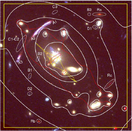
Figure 1: Image of the Abell 2667 cluster core imaged with HST in the F450W, F606W, and F814W filters. The white (thin yellow) square shows the IFU field of view, which is $54"\times 54"$. North is to the top and east is to the left. Note the strongly magnified gravitational arc north-east of the central galaxy. The white curves correspond to iso-mass contours from the lens model; the dark gray (red) line is the critical line at the redshift of the giant arc. The field of view is centered on $\alpha_{J2000}$=23:52:28.4, $\delta_{J2000}$=$-$26:05:08. At a redshift of $z=0.233$, the angular scale is $3.661$ kpc/arcsec.

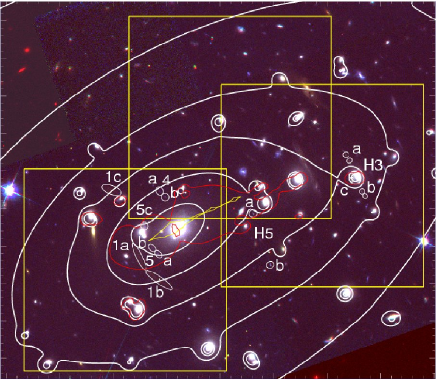
Figure 2: Image of the Abell 2390 cluster core imaged with HST in the F450W, F606W, and F814W filters. The white (thin yellow) squares correspond to the IFU field of view in different pointings. The white curves correspond to iso-mass contours from the lens model. The dark gray (red) line is the critical line at the redshift of the giant arc, labelled 1. Each square is $54"\times 54"$. North is to the top and east is to the left. The field of view is centered on $\alpha_{J2000}$=21:53:36.970, $\delta_{J2000}$=+17:41:44.66. At a redshift of $z=0.228$, the angular scale is $3.601$ kpc/arcsec.

On May $30$ and June $1$, $2001$, near-infrared J-band and H-band observations of A2667 were obtained with ISAAC on the VLT Covone et al. (2006). The total exposure times for the J and H band ISAAC data were $7.93~{}{\rm ksec}$ and $6.53~{}{\rm ksec}$, respectively. The final seeing was $0.51{\rm{}^{\prime\prime}}$ and $0.58{\rm{}^{\prime\prime}}$ in the J and H bands, respectively.

III.2 VIMOS Spectra

The massive galaxy clusters A2667 and A2390 were observed with VIMOS, between June $27$ and $30$, 2003 Covone et al. (2006); Jullo et al. (2007). The IFU is one of three modes available on VIMOS, and consists of 4 quadrants, each containing 1600 fibers. We used an instrumental setup in which each fiber covered a region of $0.67^{\prime\prime}$ in diameter. A single pointing covered a $54^{\prime\prime}\times 54^{\prime\prime}$ region of the sky. Roughly $10\%$ of the IFU field of view is unresponsive because of incomplete fiber coverage. A low resolution blue (LR-Blue) grism was used, covering the wavelength range $3500{{\rm\AA}}$ to $7000{{\rm\AA}}$ with spectral resolution $R\approx 250$ and dispersion $5.355{{\rm\AA}}/{\rm pixel}$. The FWHM of the axion-decay line is $195{\rm\AA}~{}\sigma_{1000}~{}m_{{\rm a},{\rm eV}}^{-1}$, and so the LR-Blue grism can resolve this line, without spreading a faint signal over too many wavelength pixels. Unfortunately, because spectra from contiguous pseudo-slits (sets of 400 spectra) on the CCD overlap, the first and last $50$ pixels on most of the raw spectra are unusable, reducing the spectral range to $4000{\rm\AA}-6800{\rm\AA}$, corresponding to an axion mass-range of $4.5\leq m_{{\rm a},{\rm eV}}\leq 7.7$ at the nearly identical redshifts ($z\approx 0.23$) of the two clusters. Further observational details are discussed in Ref. Covone et al. (2006).

The total exposure time for each cluster was $10.8~{}{\rm ksec}$ ($4\times 2.70~{}{\rm ksec}$ exposures). Calibration frames were obtained after each of the exposures, and a spectrophotometric standard star was observed. In order to compensate for the presence of a small set of bad fibers, we used an offset between consecutive exposures. At a redshift of $z=0.233$ (A2667), the IFU covers a physical region of $198~{}{\rm kpc}\times 198~{}{\rm kpc}$ in the plane of the cluster. At a redshift of $z=0.228$ (A2390), the IFU covers a physical region of $195~{}{\rm kpc}\times 195~{}{\rm kpc}$.

III.3 Reduction of IFU data

If axions exist and are present in the halos of massive galaxy clusters, a distinct spectral feature will appear in VIMOS-IFU data. At a rest-frame wavelength $\lambda_{{\rm a}}$, we will observe a spatially extended emission line whose intensity traces the projected dark-matter density. Revealing such a faint, spatially extended signal requires great care in correcting for fiber efficiency and in subtracting the sky background, because the instrument itself can impose spatial variation in the sky background through varying IFU fiber efficiency.

The VIMOS-IFU data were reduced using the VIMOS Interactive Pipeline Graphical Interface (VIPGI), and the authors’ own routines Scodeggio et al. (2005). References Zanichelli et al. (2005); Covone et al. (2006) give both a detailed description of the methods and an assessment of the quality of VIPGI data reduction. The reduction steps that precede the final combination of the dithered exposures into a single data cube are performed on a quadrant by quadrant basis. The main steps are the following Covone et al. (2006); D’Odorico et al. (2003); Scodeggio et al. (2005); Zanichelli et al. (2005); Horne (1986): extract spectra from the raw CCD data at each pointing, calibrate wavelength, remove cosmic rays, determine fiber efficiencies, subtract the sky background, and calibrate flux.

The exposures were bias subtracted. Cosmic-ray hits were removed with an efficient automatic routine based on a $\sigma$-clipping algorithm, which exploits the fact that cosmic-ray hits show strong spatial gradients on the CCD Zanichelli et al. (2005), in contrast to the smoother spatial behavior of genuine emission lines. In Ref. Bershady et al. (1991), spectra were obtained using a limited number of long-slit exposures, so the removal of a small number of incorrectly identified cosmic-ray hits could thwart a search for line emission from decaying axions. An axion-decay line, however, must smoothly track the density profile of the cluster. Our spectra are highly spatially-resolved, and so cosmic-ray hits can be removed safely using our cleaning algorithm. Using the raw CCD spectral traces, we verified that the signals removed by the cleaning algorithm bore the distinctive visual signatures of cosmic-ray hits.

VIPGI usually determines fiber efficiencies by normalizing to the flux of bright sky lines; this technique yielded data cubes with prominent bright and dark patches (each covering $\sim 20\times 20$ fibers). It is conceivable that an accidental correlation of these patches with the cluster density profile could lead to a spurious axion signal. To avoid this possibility, we measured fiber efficiency using high signal to noise continuum arc-lamp exposures (analogous to flat-fielding for images and henceforth referred to as flat-fielding). The resulting flat-fielded data cubes were much less patchy, and were thus used for all subsequent analysis.

The VIMOS IFU does not have a dedicated set of fibers to determine the sky-background level. VIPGI usually determines the sky statistically at each wavelength. VIPGI first groups the fibers in each quadrant into three sets according to the shape of a user selected sky-emission line, and then takes the statistical mode of the counts in each set and subtracts it from the counts measured in each fiber in the set Scodeggio et al. (2005). Although axions (and thus their decay luminosity) trace the centrally peaked density profile of the cluster, the average decay luminosity would be wiped out by this procedure, and lead to a spurious depression in measurements of $\xi$. The sky subtraction implemented in VIPGI is thus unsuitable for our axion search and was not applied. A customized sky-subtraction was applied, as discussed in Section IV.2.

Flux is calibrated separately for each IFU quadrant, using observations of a standard star. Finally, the four fully reduced exposures are combined. The final data cube for A2667 is made of 6806 spatial elements, each one containing a spectrum from $3500{\rm\AA}$ to $7000{\rm\AA}$, and covers a sky area of 0.83 arcmin², centered $5$ arcsec south-west of the brightest cluster galaxy. The final data cube for A2390 is made of $24,645$ spatial elements, each one containing a spectrum from $3500{\rm\AA}$ to $7000{\rm\AA}$, and covers a sky area of $3.11$ arcmin², centered $15$ arcsec north-east of the brightest cluster galaxy. The median spectral resolution is $\simeq 18\rm{\AA}$. For further discussion of the process used to generate the data cubes, see Refs. Zanichelli et al. (2005); Covone et al. (2006).

After producing data cubes in VIPGI, we passed these data cubes to a secondary routine that searches for emission from axion decay and estimates the noise in our spectra. The most obvious source of error is Poisson counting noise. The number of photons observed at wavelength $\lambda$ in the $\rm{j}^{\rm{th}}$ spatial bin is just $N_{\lambda,j}=E\left[F_{\lambda,j}/(hc/\lambda)\right]\delta t\delta\lambda\delta A$, where $\delta A=51.2\rm{m}^{2}$ is the collecting area of the Mélipal telescope, $\delta\lambda=5.355\rm{\AA}$ is the dispersion of a single VIMOS spectral pixel, $\delta t$ is the integration time, $F_{\lambda,j}$ is the flux in the j^th pixel at wavelength $\lambda$, and $E$ is the end to end mean efficiency of VIMOS mounted at Mélipal. The Poisson counting noise is $\delta N_{\lambda,j}\approx\sqrt{N_{\lambda,j}}$, and so $\delta I_{\lambda,j}\approx I_{\lambda,j}/\sqrt{N_{\lambda,j}}$. A secondary error source is flux contamination from neighboring pixels. To include this error, we use the $5\%$ estimate of Ref. Zanichelli et al. (2005), calculate the ‘leakage’ contribution to noise at each pixel by taking the mean flux of all the nearest neighboring pixels, and multiply it by $5\%$. We also use time-logged measurements of the CCD bias and dark-current, with the appropriate integration time, to calculate the additional noise from these sources. Finally we estimate the flat-fielding noise using the rms difference between different sets of efficiency tables. These errors are added in quadrature to obtain a data cube of the estimated errors in specific intensity.

In Refs. Ressell (1991); Bershady et al. (1991), slit locations were chosen to avoid the locations of known galaxies, as well as regions that showed statistical evidence for faint galaxies Bershady (2005). Likewise, we masked out IFU fibers that fell on the locations of individual bright sources. Bright sources were identified in each cluster image by tagging pixels where the image intensity exceeded the median by more than $1\sigma$ and masking IFU fibers that fell on these pixels. Practically, this means that $40\%$ of the fibers in each data cube are left unmasked. The images used to generate this mask are broadband, and so this masking technique will not mask out an axion-decay signal. The accidental inclusion of galaxies could conceivably lead us to erroneously attribute their emission to axion decay. This is unlikely, given that the spectra of cluster galaxies are dominated by continuum emission and line absorption. If we see an indication of emission due to line decay, however, we may have to revise our masking criteria to take account of this possibility. As we shall see later, we imposed upper limits to axion decay, and can safely use the chosen masking criterion. The resulting masks were visually inspected to verify that most of the masked fibers fall near galaxies. To extract the density dependent component of the cluster spectra, we apply a mass map obtained from gravitational lensing observations.

IV Analysis

IV.1 Strong Lensing and Cluster Mass Maps

To model the mass distribution of A2667 and A2390, we used both a cluster mass-scale component (representing the contribution of the dark-matter halo and the intracluster medium) and cluster-galaxy mass components as in Refs. Kneib et al. (1996a); Smith et al. (2005). Cluster galaxies were selected according to their redshift (when available, in the inner cluster region covered with VIMOS spectroscopy) or their color, thus selecting galaxies belonging to the cluster red sequence. For A2667, ISAAC images were used to determine J-H colors, whereas for A2390, HST images were used to determine I-V colors. The lensing contribution from more prominent foreground galaxies was also included, rescaling their lensing properties using the appropriate redshift.

All model components were parameterized using a smoothly truncated pseudo-isothermal mass distribution model (PIEMD) Kassiola and Kovner (1993), which avoids both the unphysical central-density singularity and the infinite spatial extent of the singular isothermal model.

The galaxy mass components were chosen to have the same position, ellipticity and orientation as their corresponding images. The K-band luminosity of the galaxies was computed, assuming a typical E/S0 spectral energy distribution (redshifted but uncorrected for evolution of constituent stellar populations). Their masses were estimated using the K-band luminosity, calculated assuming a global mass to light ratio ($M/L$) and the Faber-Jackson relation Faber and Jackson (1976). The final mass model is made of 70 components, including the large scale cluster halo and the individual galaxies.

Using the LENSTOOL ray-tracing code Kneib (1993) with the HST images, we iteratively implemented the constraints from the gravitational lenses. Lensing mass models with $\chi^{2}\leq 1$ were found by fitting the ellipticity, orientation, center, and mass parameters (velocity dispersion, core radius, and truncation radius) of the cluster scale component, as well as the truncation radius and velocity dispersion of the ensemble of cluster galaxies, using scaling relations for early-type galaxies Natarajan and Kneib (1997). Cluster galaxy redshifts were measured using the IFU data Covone et al. (2006). The bright central galaxy and several galaxies near the locations of strong-lensing arcs were modeled separately from the ensemble. The resulting cluster density maps for A2667 and A2390 are shown in Figs. 3 and 4 Covone et al. (2006); Jullo et al. (2007). Statistical errors in the mass model parameters were propagated through the relevant code to produce a fiber by fiber map of statistical errors in $\Sigma$. These maps were then used to weight different IFU fibers and thus maximize the signal to noise ratio of any putative line emission from axion decay.

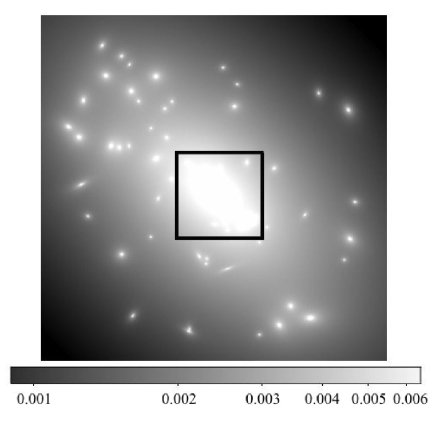
Figure 3: Mass map of A2667. The intensity of the image scales with density (in units of $10^{12}M_{\odot}~{}\rm{pix}^{-2}$), where $1~{}\rm{pix}=0.50"$. A density scale is provided on the bottom of the image. The horizontal extent of this map is $222.6^{\prime\prime}$. The vertical extent is $200.0^{\prime\prime}$. The thick black line indicates the spatial extent of the IFU head on the mass map.

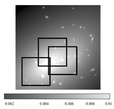
Figure 4: Mass map of A2390. The intensity of the image scales with density (in units of $10^{12}M_{\odot}~{}\rm{pix}^{-2}$), where $1~{}\rm{pix}=0.50"$. A density scale is provided on the bottom of the image. The horizontal spatial extent of the map is $157.5"$. The vertical extent is $150.0^{\prime\prime}$. The thick black lines indicate IFU pointings used to construct our data cubes.

IV.2 Extraction of One Dimensional Spectra

Using density maps of A2667 and A2390, we can optimally weight averages over fibers to maximize the contribution from high density regions of the cluster. This maximizes the signal to noise ratio of our axion search by emphasizing IFU fibers where maximum signal from axion decay is expected. These maps allow us to separate emission correlated with the mass profile of the cluster, which could be due to axion decay, from a sky background that we assume to be spatially homogeneous. Our technique is an IFU generalization of the long-slit ‘on-off’ sky-subtraction technique presented in Refs. Ressell (1991); Bershady et al. (1991). The real sky background is certainly not perfectly homogeneous, but by making this assumption, we are being maximally conservative. With our reduction method, any density correlated spatial dependence in the sky background will show up as putative emission from axion decay. If evidence for a signal is seen, we will have to be careful to avoid being confused by sky line emission. The projected surface density of the cluster at the location in the lens plane associated with the $i^{\rm{th}}$ fiber is denoted $\Sigma_{12,i}$. Assuming that the only spatially dependent signal comes from axions, we can then model the actual intensity $I_{\lambda,i}^{\rm{mod}}$ at a given wavelength $\lambda$ and spatial pixel $i$ as $I_{\lambda,i}^{\rm{mod}}=\langle I_{\lambda}/\Sigma_{12}\rangle\Sigma_{12,i}+b_{\lambda}$, where $b_{\lambda}$ represents the contribution of a spatially homogeneous sky signal, and $I_{\lambda,i}$ is the specific intensity in the $i^{\rm{th}}$ fiber at wavelength $\lambda$. Since the signal from axion decay is bounded from above by the total component of the signal proportional to $\Sigma_{12,i}$, a measurement of $\langle I_{\lambda}/\Sigma_{12}\rangle$ will either provide evidence of axion decay, or impose an upper limit on $\langle I_{\lambda}/\Sigma_{12}\rangle_{\rm{axion}}$. Using a simple linear fit to separate the sky background from signal, we extract the array $\langle I_{\lambda}/\Sigma_{12}\rangle$ from each cluster data cube.

At a small number of wavelengths, this yielded negative (unphysical) values for one or both fitted parameters. To avoid this, we fit for $\langle I_{\lambda}/\Sigma_{12}\rangle$ and $b_{\lambda}$, subject to the obvious constraints $\langle I_{\lambda}/\Sigma_{12}\rangle\geq 0$ and $b_{\lambda}\geq 0$, estimating errors $\sigma_{\lambda,i}$ as described in Section III.3. Estimated errors in $\Sigma_{12}$ were also included in the fit. Residuals from the best fit are due to flux noise, imperfect masking of galaxies, and variations in fiber efficiency unaccounted for by the flat-fielding procedure. As can be seen directly from the unconstrained linear-least-squares solutions for the parameters $\langle I_{\lambda}/\Sigma_{12}\rangle$ and $b_{\lambda}$, this procedure places higher weights on those VIMOS fibers that fall on higher density portions of the cluster. In essence, we used our knowledge of the cluster density profile to extract only the information that interests us, namely, that part of the emission that is correlated with the cluster’s mass density profile. At some wavelengths, the best fit is $\langle I_{\lambda}/\Sigma_{12}\rangle=0$ with very low noise. We verified that these wavelengths coincide with those at which a naive linear fit yielded negative values for $\langle I_{\lambda}/\Sigma_{12}\rangle$. Thus there is no evidence for density correlated emission at these wavelengths. At these wavelengths, the emission due to axion decay is bounded from above by the brightness of the sky background, and so we used $\langle I_{\lambda}/\Sigma_{12}\rangle\leq b_{\lambda}/\langle\Sigma_{12}\rangle$ to obtain a conservative upper limit on the flux. Decaying axions will produce line emission, so it might seem that an additional continuum subtraction might be in order. The continuum component of the sky background, however, is already subtracted using the techniques discussed, and an additional continuum subtraction step would be erroneously aggressive.

As a test of our sky-subtraction technique, we also reimplemented the sky-subtraction technique of Ref. Bershady et al. (1991) and implemented an ‘on-off’ subtraction by defining fibers further than $23^{\prime\prime}$ (A2667) or $72^{\prime\prime}$ (A2390) from the cluster center (defined by the highest density point in the density maps) as ‘sky’ fibers, spatially averaging the flux of these sky fibers at each wavelength, and subtracting the resulting sky spectrum from each pixel in the ‘on’ cluster region. In this case, sky emission was directly estimated from the data rather than modeled. In this case, the best fit for the signal is given by

$$\left\langle\frac{I_{\lambda}}{\Sigma_{12}}\right\rangle=\frac{\sum_{i}\frac{I_{\lambda,i}\Sigma_{12,i}}{\sigma_{\lambda,i}^{2}}}{\sum_{i}\frac{\Sigma_{12,i}^{2}}{\sigma_{\lambda,i}^{2}}},$$ (5)

where $i$ is a label for the density at the location of a given IFU fiber, and $\sigma_{\lambda,i}$ is the error in the specific intensity.

In the case of A2667, even the fibers furthest from the cluster center fall on portions of the cluster where emission due to axion decays will be of the same order of magnitude as at the center. The sky-subtraction technique of Ref. Bershady et al. (1991) is thus entirely inappropriate for our data on A2667, as it will subtract out a substantial fraction of any signal and return unjustifiably stringent limits to emission from axion decay.

For A2390, the effective field of view is much larger, and so the emission expected from axion decays in the outer fibers is much less. Over most of the wavelength range of our data for A2390, the different sky-subtraction techniques agreed to within a factor of two, leading us to believe that our sky-subtraction technique is trustworthy. We used the value for $\langle I_{\lambda}/\Sigma_{12}\rangle$ obtained using our sky-subtraction technique, as it is desirable to use the same sky-subtraction method for both clusters to be self-consistent. Equation (5) and the corresponding best-fit result in the constrained case essentially yield one-dimensional cluster spectra, rescaled by the cluster density, as shown in Figs. 5 and 6. The specific intensity values in Fig. 5 were obtained by multiplying the best-fit values of $\langle I_{\lambda}/\Sigma_{12}\rangle$ from Eq. (5) by the mean $\langle\Sigma_{12}\rangle=\left(\sum_{i}\Sigma_{12,i}/\sigma_{\lambda,i}^{2}\right)/\left(\sum_{i}1/\sigma_{\lambda,i}^{2}\right)$. The plotted spectrum is thus not the best-fit spectrum at any particular fiber, but an average cluster spectrum. The signal to noise ratio of the one-dimensional spectrum appears to be higher for A2667 than for A2390, in spite of the lower effective fiber number of the data cube for A2667. We believe that this is the case because the data cube for A2390 was built using four nights of data, with slight variations in sky intensity and efficiency from night to night. The subtraction is poorest around the prominent sky line at $5577\rm{\AA}$. There is no obvious candidate for an emission line due to axion decay.

Figure 5: Average one-dimensional sky subtracted spectra of clusters A2667 and A2390. Intensity is in units of $10^{-18}~{}{\rm ergs}~{}{\rm cm}^{-2}~{}{\rm s}^{-1}~{}{{\rm\AA}}^{-1}~{}\mbox{arcsec}^{-2}$. Poorly subtracted sky emission lines at $5577\rm{\AA}$, $5894\rm{\AA}$, and $6300\rm{\AA}$ have not been removed.

Figure 6: Constraints on $\langle I_{\lambda}/\Sigma_{12}\rangle$ as a function of wavelength $\lambda$ for A2667 and A2390. CGS units for specific intensity are ${\rm ergs}~{}{\rm cm}^{-2}~{}{\rm s}^{-1}~{}{{\rm\AA}}^{-1}~{}\mbox{arcsec}^{-2}$, and $\Sigma_{12}=\Sigma/(10^{12}M_{\odot}~{}\rm{pix}^{-2})$, where $\Sigma$ is the projected mass density of the cluster, measured using strong lensing. The over-plotted dashed lines are theoretical Gaussian spectra for axion decays, with central wavelength $\lambda_{0}$, corresponding to an axion mass of $m_{\rm{a},\rm{eV}}=24,800{{\rm\AA}}(1+z)/\lambda_{0}$. The predicted amplitude is set by Eq. (4), and exceeds the measured values in both the top panel ($\xi=1.0$) and the bottom panel ($\xi=0.03$).

IV.3 Limits on the two-photon coupling of axions

The expected strength of an axion decay line is set by $m_{\rm{a},\rm{eV}}$ through Eq. (4), and the expected Gaussian line profiles are shown on top of our appropriately normalized upper limits to flux in Fig. 6 for several candidate axion masses. The narrow feature at $5577\rm{\AA}$, present in both panels of Fig. 6, arises from the imperfect subtraction of a sky emission line. In the absence of a candidate axion decay line, we proceed to put an upper limit on the coupling strength $\xi$ of an axion to two photons.

Since our best-fit values for $R_{\lambda}\equiv\langle I_{\lambda}/\Sigma_{12}\rangle$ at each wavelength come with an error estimate $\sigma_{\lambda}$, we can calculate a $95\%$-confidence limit to the line flux. We assume that the distribution of noise peaks is Gaussian, and so the probability that an axion decay associated with a particular value of $R_{\rm{a},\lambda}$ yields a measured best-fit value less than $R_{\lambda}$ is

$$P_{\lambda}=\frac{1}{\sqrt{2\pi}\sigma_{\lambda}}\int_{-\infty}^{R_{\lambda}-R_{\rm{a},\lambda}}e^{\frac{-x^{2}}{2\sigma_{\lambda}^{2}}}dx.$$ (6)

Eq. (6) yields the $95\%$-confidence limit on intensity from axion decay:

$$R_{\rm{a},\lambda}\leq R_{\lambda}+1.65\sigma_{\lambda}.$$ (7)

At those wavelengths where the best-fit value is $R_{\lambda}=0$, we have taken the roughly homogeneous intensity of the sky as a very conservative upper limit on the intracluster emission. This is many $\sigma$ above the $95\%$-confidence limit, and so at these wavelengths, we just take $R_{\rm{a},\lambda}\leq R_{\lambda}$ without making our estimate of the upper limit too conservative. Ultimately, we wish to combine the upper limits to flux from the two clusters. One of the advantages of working with two clusters at slightly different redshifts is that rest-frame wavelengths falling near sky lines (where limits to flux are generally quite poor) at one redshift may no longer fall on sky emission lines at the redshift of the second cluster. When this is the case, we excise wavelengths falling on or near sky lines from each spectrum. To account for all the flux in a given candidate axion line, in each cluster spectrum, we calculate the average intensity of non-excised data points in a $24,800\left[(1+z)\sigma/c\right]~{}{\rm\AA}~{}m_{{\rm a},{\rm eV}}$ window around a series of putative line centers spanning the probed axion mass range. We weight the noise in the usual way. Assuming that our spectra uniformly sample this bin and that flux errors are uniform across the bin, we see by integrating the Gaussian profile given in Eq. (4) that

$$R_{\rm{a},\lambda}=\frac{2.30\times 10^{-18}~{}\xi^{2}m_{{\rm a},{\rm eV}}^{7}}{(1+z_{{\rm cl}})^{4}S^{2}(z_{{\rm cl}})\sigma_{1000}}~{}{\rm cgs}.$$ (8)

If axions have the standard thermal-freezeout abundance [Eq. (1)], then the limit on the axion coupling is given by

$$\begin{array}[]{c}\xi\leq\left[\frac{\sigma_{1000}(1+z_{\rm{cl}})^{4}S^{2}(z_{\rm{cl}})m^{-7}_{\rm{a},\rm{eV}}(\lambda)R_{\rm{a},\lambda}}{2.30\times 10^{-18}~{}\rm{cgs}}\right]^{1/2}\end{array}.$$ (9)

If the cosmological axion abundance takes on some other value $\Omega_{\rm a}h^{2}$, then the limit becomes

$$\begin{array}[]{c}\xi\sqrt{\Omega_{{\rm a}}h^{2}}\leq\left[\frac{\sigma_{1000}(1+z_{\rm{cl}})^{4}S^{2}(z_{\rm{cl}})m^{-6}_{\rm{a},\rm{eV}}(\lambda)R_{\rm{a},\lambda}}{3.48\times 10^{-16}~{}\rm{cgs}}\right]^{1/2}.\end{array}$$ (10)

Since our real bins are not uniformly sampled (because of the excision of wavelengths that fall on sky emission lines) and since the errors scale with the intensity value at a given wavelength, we make a small correction to this expected value. Specifically,

$$R_{{\rm a},\lambda}=\frac{2.68\times 10^{-18}~{}\xi^{2}m_{{\rm a},{\rm eV}}^{7}}{(1+z_{{\rm cl}})^{4}S^{2}(z_{{\rm cl}})}\frac{\sum_{j\in T_{\lambda}}\frac{G_{j}}{\sigma_{j}^{2}}}{\sum_{j\in T_{\lambda}}\frac{1}{\sigma_{j}^{2}}}~{}{\rm cgs},$$

$$\mbox{where}~{}G_{j}=e^{-\frac{(\lambda_{j}/(1+z_{{\rm cl}})-\lambda_{{\rm a}})^{2}c^{2}}{2\sigma^{2}\lambda_{{\rm a}}^{2}}},$$ (11)

$T_{\lambda}$ is the set of all non-excised wavelengths lying within the bin centered at wavelength $\lambda$, and $j$ labels wavelengths. The quality of sky background subtraction may vary as a result of spatial and temporal variations in the sky background from night to night. If it is not due to axion decay, the density correlated emission might also genuinely vary between clusters. The quantity $R_{\rm{a},\lambda}$, however, will by definition be independent of these factors. A simple error weighted mean of the upper limits obtained from the two clusters would thus erroneously increase the upper limit placed on $\xi$. If two clusters yield different best-fit values for $R_{\lambda}$, $R_{\rm{a},\lambda}$ must be bounded from above by the lesser of these two. By comparing upper limits to $R_{\lambda}$ obtained from A2390 with those obtained from A2667 and choosing the lowest value at each wavelength, we obtained the maximum values of $R_{\rm{a},\lambda}$ consistent with the data. We then applied Eq. (11) to obtain an upper limit on $\xi$ consistent with the spectra of both clusters. To account for variation in the upper limits to $\xi$ arising from systematic errors in the cluster mass profiles, we repeated the preceding analysis, drawing $\Sigma_{12,i}$ from the best-fit NFW (Navarro, Frenk, and White) and King profiles to the cluster mass profiles.

Analytic expressions for the volumetric and surface mass density for NFW and King profiles are reviewed in Appendix A. We determined the mass profile parameters ($a$ and $\sigma$ for King profiles, $c$ and $\sigma$ for NFW profiles) by fitting to our strong-lensing density maps. Using these different density profiles and assuming that the mass fraction in axions is $x_{\rm{a}}=\Omega_{\rm{a}}h^{2}/(\Omega_{{\rm m}}h^{2})$, we obtain limits to $\xi$. The cluster density at the location of a given IFU fiber varies from profile to profile, and so different fibers receive higher weights when a one-dimensional spectrum is extracted. This explains the variation in upper limits to $\xi$ that arises when different density profiles are assumed. We show the most conservative (with respect to choice of density profile) limit on $\xi$ (assuming the thermal-freezeout abundance of axions) at each candidate axion mass in Fig. 7. The upper limits to $\xi$ in adjacent points along the $m_{\rm{a},\rm{eV}}$ axis are correlated due to overlapping bins. The narrow black arrows near $m_{\rm{a},\rm{eV}}=5.43$ and $4.83$ mark sharp night-sky lines at $\lambda=5577\rm{\AA}$ and $\lambda=6300{\rm\AA}$, where sky subtraction is unreliable and useful limits to $\xi$ cannot be obtained. Limits on $\xi$ and specific intensity at the putative line center are displayed for several candidate masses in Table 1. Our data rule out the canonical DFSZ and KSVZ axion models in the mass window $4.5\leq m_{\rm{a},\rm{eV}}\leq 7.7$, as seen in Fig. 8. However, theoretical uncertainties motivate the search for axions with values of $\xi$ smaller than those allowed by the canonical KSVZ and DFSZ models.

If we relax the assumption that the cosmological axion abundance be given by Eq. (1), then our null search implies the bound, shown in Fig. 9, to the combination $\xi(\Omega_{\rm a}h^{2})^{1/2}$. We see that if $\xi\sim 10^{-1}$, as is the case in the KSVZ model, then our results imply an upper limit $\Omega_{\rm a}h^{2}\mathrel{\hbox{\hbox to0.0pt{\lower 2.36806pt\hbox{$\sim$}\hss} \kern-3.00003pt\raise 1.72218pt\hbox{$<$}}}10^{-4}$ in our mass range, roughly two orders of magnitude stronger than CMB/LSS limits Hannestad et al. (2005), which probe densities down to $\Omega_{\rm a}h^{2}\sim 10^{-2}$.

IV.4 Revision of past telescope constraints to axions

As can be seen from Eq. (4), and from the fact that the mass fraction of the cluster in axions is $x_{\rm{a}}=\Omega_{\rm{a}}h^{2}/(\Omega_{{\rm m}}h^{2})$, the upper limit on $\xi$ derived from a given upper limit on flux depends on the cluster mass model used and the cosmological parameters assumed. References Bershady et al. (1991); Ressell (1991) date to a time when the observationally favored cosmology was sCDM (Standard Cold Dark Matter: $h=0.5$, $\Omega_{{\rm m}}=1.0$, $\Omega_{\Lambda}=0$). Moreover, the King profiles assumed in those analyses of A2218, A2256, and A1413 were based on available x-ray emission profiles of the chosen clusters Ressell (1991); Bershady et al. (1991) (and references therein). The advent of modern x-ray instruments has improved x-ray-derived cluster mass profiles, and gravitational-lensing studies have allowed measurements of cluster mass profiles, free of the dynamical assumptions required to obtain a density profile from an x-ray temperature map. The quoted upper limits of Refs. Ressell (1991); Bershady et al. (1991) must thus be rescaled, and we have done so up to an ambiguity in slit placement for A2218; details are discussed in Appendix B and the rescaled limits from past work are shown alongside our own in Fig. 7. Our limits improve on the rescaled limits of Ref. Ressell (1991); Bershady et al. (1991) by a factor of $2.1-7.1$. Our final measurement of $\langle I_{\lambda}/\Sigma_{12}\rangle$ is only noise limited at a small fraction ($\simeq 10\%$) of the available wavelength range. The dominant uncertainty is systematic and comes from sky subtraction. The expected improvement estimated in the introduction assumed that we are limited by Poisson noise in the measured flux, and is thus naive.

Figure 7: Upper limits to the two-photon coupling parameter $\xi$ of the axion, derived directly from upper limits to the intracluster flux of A2667 and A2390. Our data exclude the shaded region. The solid and dashed lines show the upper limits reported in Refs. Ressell (1991); Bershady et al. (1991), adjusted (optimistically and pessimistically) for differences between today’s best-fit measurements of the cosmological parameters/cluster mass profiles and the assumptions in Refs. Ressell (1991); Bershady et al. (1991). Details are discussed in Appendix B. The mass range $4.5~{}{\rm eV}\leq m_{{\rm a}}\leq 7.7~{}{\rm eV}$ arises from the $4000\rm{\AA}$–$6800\rm{\AA}$ usable wavelength range of VIMOS, which is smaller than that of the KPNO spectrograph used in Ref. Bershady et al. (1991). The narrow black arrows near $5.43~{}{\rm eV}$ and $4.83~{}{\rm eV}$ mark the sharp night-sky lines at $5577\rm{\AA}$ and $6300{\rm\AA}$, where sky subtraction is unreliable and useful limits to $\xi$ cannot be obtained. The shaded exclusion region is derived by applying the cluster density profile (strong-lensing map, best-fit NFW profile, or best-fit King profile) at each candidate axion mass that yields the most conservative upper limit on $\xi$.

Table 1: Upper limits to central line intensity and $\xi$ at several candidate axion masses, derived directly from sky subtracted spectra of A2667 and A2390.

$m_{\rm{a},\rm{eV}}$	$\left\langle I_{\lambda}/\Sigma_{12}\right\rangle\left\langle\Sigma_{12}\right\rangle$ (cgs)	$\xi$
$4.5$	$1.83\times 10^{-19}$	$7.17\times 10^{-3}$
$5$	$6.04\times 10^{-19}$	$9.00\times 10^{-3}$
$6$	$8.74\times 10^{-19}$	$5.72\times 10^{-3}$
$6.5$	$9.91\times 10^{-19}$	$4.60\times 10^{-3}$
$7$	$9.13\times 10^{-19}$	$3.41\times 10^{-3}$
$7.5$	$1.11\times 10^{-18}$	$2.95\times 10^{-3}$
$7.65$	$8.96\times 10^{-19}$	$2.47\times 10^{-3}$

Figure 8: Comparison of existing limits to the two-photon coupling of a $4.5~{}\rm{eV}-14~{}\rm{eV}$ axion with the projected sensitivity of our proposed observations of lensing cluster RDCS 1252 ($z=1.237$). Flux limits and density profiles were assumed to be the same as those of A2667/A2390. The best existing upper limits to $\xi$ in the higher mass window come from limits to the Diffuse Extragalactic Background Radiation (DEBRA), and were rescaled for consistency with today’s best-fit $\Lambda$CDM parameters and recent measurements Turner (1987); Overduin and Wesson (1993). The limits reported in this and previous work, derived using optical spectroscopy of galaxy clusters, are shown for comparison Ressell (1991); Bershady et al. (1991). Regions inaccessible due to night-sky emission lines are marked with narrow black arrows. The two solid horizontal lines indicate the predictions of the DFSZ and KSVZ axion models; the downward arrows indicate that $\xi$ is theoretically uncertain.

Figure 9: Limits on the combination $\xi\left(\Omega_{{\rm a}}h^{2}\right)^{1/2}$, derived directly from upper limits to the intracluster flux of A2667 and A2390. Our data exclude the shaded region. Data analysis proceeds as in the thermal case, but appropriate (more general) expressions for the intensity $I_{\lambda}$ are used. These constraints do not depend on the assumption that axions are produced thermally at early times.

Previous cluster searches for axions used long-slit spectroscopy. Our use of IFU data is novel, and it is conceivable that peculiarities of the data-reduction techniques used in IFU spectroscopy may affect the sensitivity of our search. To explore this possibility, we have conducted a simulation.

IV.5 Simulation of Analysis Technique

We simulate axion-decay emission in our data cube for A2667, using Eq. (4) and our lensing derived projected density maps. We did this at a range of $10$ candidate axion masses spanning the full mass range of our search. We used $3$ or $4$ different values of $\xi$ at each candidate mass. The first value was chosen to be slightly below ($5-10\%$) the limit on $\xi$ set by preceding techniques, while the second was chosen to be slightly above the upper limit. The third and fourth values were chosen to be in considerable (factors of $2$ and $10$, respectively) excess of the upper limit. For all simulated axion masses, visual inspection of the data cube yields clear evidence for the inserted line when $\xi$ exceeds the imposed upper limit. An example is shown in Fig. 10. After inspecting the data cubes visually, we applied the routines used for the preceding analysis to produce one-dimensional spectra for each cube. We then applied the same routine used to extract upper limits to $\xi$ to recover the simulated $\xi$ value. When the simulated value of $\xi$ exceeded the upper limit, we recovered the correct answer in all cases to a precision of $5-10\%$. This leads us to believe that our technique is robust and our upper limits reliable. References Ressell (1991); Bershady et al. (1991) supplement upper limits to $\xi$ derived directly from flux limits with limits obtained from a cross-correlation analysis. We do the same, using our data on A2667 and A2390.

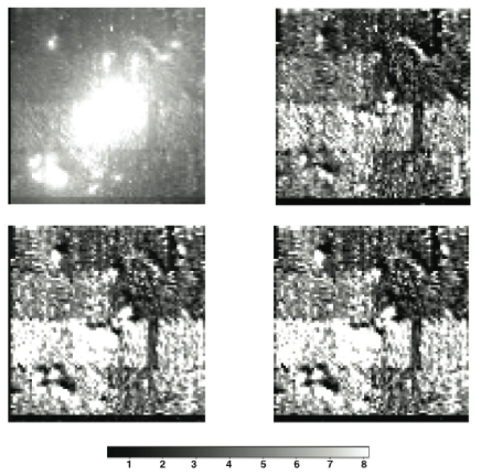
Figure 10: The upper left panel of this figure shows a simulated $4255.2\rm{\AA}$ slice of the A2667 IFU data cube, with an axion-decay emission line inserted corresponding to $m_{\rm{a},\rm{eV}}=7.2$ and $\xi=0.011$. The flux scale is in units of $10^{-18}~{}\rm{erg}~{}\rm{s}^{-1}~{}\rm{cm}^{-2}~{}\rm{\AA}^{-1}$. This slice, which lies at the expected line center, shows evidence of the inserted axion line. The resulting ‘emission’ clearly traces the cluster mass density profile. The lower left panel of this figure shows a simulated slice of the same data cube, but at $5267.2\rm{\AA}$, well away from the line center. As expected, no signature of axion emission is present this far away in wavelength from the line center. The upper/lower right panels of this figure show $4255.2\rm{\AA}$/ $5267.2\rm{\AA}$ slices, respectively, of the actual A2667 IFU data cube used for our analysis.

IV.6 Cross-Correlation Analysis

If there is an emission line at the same wavelength in the rest frame of both clusters, the function

$$g(l)=\frac{\int I_{1}(x)I_{2}(x+l)dx}{\left[\int I_{1}^{2}(x)dx\int I_{2}^{2}(x)dx\right]^{1/2}},$$ (12)

will have a peak at the lag $l_{0}=\ln{\left[\left(1+z_{{\rm A}2667}\right)/\left(1+z_{{\rm A}2390}\right)\right]}$, where $x=\ln{\lambda}$, $I_{1}(x)$ and $I_{2}(x)$ are the specific intensities of galaxy clusters A2667 and A2390, and $z_{{\rm A}2667}$ and $z_{{\rm A}2390}$ are their redshifts Ressell (1991); Bershady et al. (1991). A statistically significant peak in $g(l)$ would indicate the existence of an intracluster emission line at unknown wavelength (and correspondingly unknown axion mass), which could then be searched for more carefully in the individual spectra. Peaks due to noise may arise either due to the roughly Gaussian fluctuations in flux of the individual spectra, or due to imperfectly subtracted flux around sharp sky emission lines. It is thus appropriate to mask out bright sky lines. If we assume that the distribution of remaining noise peaks is Gaussian, then the probability that a cross-correlation peak with height greater than or equal to $s$ is due to noise is Ressell (1991); Bershady et al. (1991)

$$P(\geq s)=\int_{s}^{\infty}\frac{e^{-x^{2}/(4\sigma_{g}^{2})}dx}{\sqrt{\pi}\sigma_{g}}=1-\mbox{Erf}\left(\frac{s}{2\sigma_{g}}\right).$$ (13)

Here, $\sigma_{g}$ is the rms value of the antisymmetric component of $g(l)$ and provides an estimate of the correlation due to noise, since a Gaussian signal leads to a symmetric correlation function Ressell (1991); Tonry and Davis (1979). Equation (13) determines the statistical significance of peaks in $g(l)$. Our analysis of correlated spectra follows the treatment of Ref. Tonry and Davis (1979). We calculate $g(l)$ using the sky subtracted one-dimensional spectra of A2667 and A2390. With a cross-correlation technique, we are able to perform a blind search for cluster rest-frame emission. We find no statistically significant ($>2\sigma_{g}$) cross-correlation peaks, as shown in Fig. 11.

Figure 11: Cross-correlation function $g(l)$ between sky subtracted spectra of clusters A2667 and A2390. No peaks with the desired statistical significance were seen, at the desired lag or elsewhere. A single cross-correlation peak is near the expected lag $l=0.00498$ for an intracluster emission line common to A2667 and A2390. However, it is not statistically significant.

Table 2: Upper limits to $\xi$ at several candidate axion masses, obtained from a simulation of the cross-correlation method, using spectra of A2667 and A2390.

$m_{\rm{a},\rm{eV}}$	$\xi$
$4.5$	$2.73\times 10^{-2}$
$5$	$1.08\times 10^{-2}$
$6.0$	$9.35\times 10^{-3}$
$6.5$	$6.90\times 10^{-3}$
$7$	$4.44\times 10^{-3}$
$7.5$	$4.31\times 10^{-3}$
$7.65$	$2.16\times 10^{-2}$

We simulate our cross-correlation based search for an intracluster line in order to set alternative upper limits to $\xi$ Ressell (1991); Bershady et al. (1991). The limits reported in Ref. Bershady et al. (1991) were obtained using this technique. In our simulation, we introduced ‘fake’ axion decay lines into both spectra and calculated the resulting $g(l)$ for a variety of values $m_{\rm{a},\rm{eV}}$, thus simulating the cross-correlation search for evidence of intracluster emission. $\xi$ was initially set to a value for which a very significant peak in $g(l)$ appeared, and then ramped down until the peak at $l_{0}$ ceased to be statistically significant; that is, until $P(s)>5\%$. At that point, an upper limit on $\xi$ was set. The cross-correlation peaks due to the axion line are well fit by Gaussian curves throughout the $m_{\rm{a},\rm{eV}}-\xi$ parameter space. Since the cross-correlation function includes the contribution of flux away from the line center, rebinning was unnecessary.

To further distinguish between signal and noise peaks, we follow Ref. Ressell (1991) in using the usual criterion, $|l-l_{0}|\leq\sigma$, where $\sigma$ is the width of the best Gaussian fit to $g(l)$ around a cross-correlation peak. We use this criterion in both the simulation and the cross-correlation searchRessell (1991). The resulting limits to $\xi$ at a series of candidate axion masses are shown in Table 2, and are on average a factor of $\sim 1.5$ less stringent than those derived directly from flux.

One aspect of the correlation analysis of Ref. Ressell (1991) is troubling. Two noisy, imperfectly sky subtracted spectra were correlated to search for a signal. The analysis of Ref. Ressell (1991), however, uses one real spectrum (containing noise and an imperfectly subtracted sky-background signal) with an artificial axion line inserted, and a second, noiseless, template spectrum, containing only the artificial axion line, but no imperfectly subtracted sky component. Thus, the method simulated in Ref. Ressell (1991) is not the same as the method used to actually search for evidence of an intracluster line, and by artificially reducing the noise budget of the simulation, could lead to artificially stringent constraints. The appropriate way to simulate the cross-correlation analysis is to correlate two real spectra with artificial axion lines inserted, as we have done. Our data also place limits on the decay of other relics.

IV.7 Sterile neutrinos

Our data might also be used to constrain the decay rate of other $\sim 5~{}{\rm eV}$ relics, such as sterile neutrinos Dodelson and Widrow (1994); Dolgov and Hansen (2002); Shi and Fuller (1999); Asaka et al. (2006). Although the prevailing paradigm places the sterile-neutrino mass in the keV range, some experimental data can be fit by introducing a hierarchy of sterile neutrinos, at least one of which is in the $1-10~{}{\rm eV}$ range and could oscillate to produce photons in our observation window de Gouvea (2005); de Gouvea and Pena-Garay (2001). In our notation and in the $m_{e^{-},\mu,\tau}\ll m_{s}$ limit (where $m_{s}$ is the sterile-neutrino mass), the intensity of this signal is

$$\left\langle\frac{I_{\lambda,{\rm s}}}{\Sigma_{12}}\right\rangle=2.4\times 10^{-18}\frac{Bm_{{s},{\rm eV}}^{8}\exp{\left[-\left(\lambda_{r}-\lambda_{{\rm s}}\right)^{2}c^{2}/\left(2\lambda_{{\rm s}}^{2}\sigma^{2}\right)\right]}}{\sigma_{1000}(1+z_{{\rm cl}})^{4}S^{2}(z_{{\rm cl}})}{\rm cgs},$$ (14)

where $B$ is a model-dependent normalization factor, the oscillation is parameterized by a cumulative mixing angle $\theta$, and the additional power of mass arises from the late-time abundance of sterile neutrinos Abazajian et al. (2001a):

$$\Omega_{{\rm s}}h^{2}=0.3\times m_{s,{\rm eV}}^{2}\sin^{2}2\theta.$$ (15)

The flux limits in Table 1 impose the constraints $B\leq 8.03\times 10^{-5},~{}1.14\times 10^{-4},~{}9.41\times 10^{-5},~{}3.82\times 10^{-5},~{}2.28\times 10^{-5},1.16\times 10^{-5},~{}8.12\times 10^{-6}$, and $5.61\times 10^{-6}$ for sterile-neutrino masses of $m_{s,{\rm eV}}=4.50,~{}5.00,~{}5.50,~{}6.00,~{}6.50,~{}7.00,~{}7.50$, and $7.65$, respectively. In conventional models, $B=\sin^{4}{\left(2\theta\right)}/10^{11}$. The parameter $B$ encodes the effects of both the early-universe production and the decay of sterile neutrinos, which occurs at the rate $\Gamma_{s\to\nu+\gamma}=6.8\times 10^{-38}{s}^{-1}m_{s,{\rm eV}}^{5}\sin^{2}{2\theta}$ Pal and Wolfenstein (1982); De Rujula and Glashow (1980); Abazajian et al. (2001b); Barger et al. (1995). By definition, $B\leq 10^{-11}$, and so optical data only constrain sterile neutrinos if some novel mechanism increases the oscillation rate $\Gamma_{s\to\nu+\gamma}$ by many orders of magnitude. The sharp disparity between x-ray and optical constraints results from the $\Gamma\propto m_{s}^{5}$ scaling of the decay rate.

IV.8 Future Work

We have demonstrated the utility of applying integral field spectroscopy in concert with lensing data to search for axions in $z\simeq 0.2$ galaxy clusters. Our technique could also be profitably applied to higher redshift galaxy clusters. Although flux falls off as $I_{\lambda}\propto(1+z_{{\rm cl}})^{-4}$, the fact that we are pushing to a higher mass range $m_{{\rm a},{\rm eV}}=24,800{\rm\AA}\left(1+z_{{\rm cl}}\right)/\lambda_{{\rm a}}$ increases the expected signal. Since $I_{\lambda}\propto m_{{\rm a},{\rm eV}}^{7}$, the expected signal actually increases as $I_{\lambda}\propto\left(1+z_{{\rm cl}}\right)^{3}$. The most distant known lensing cluster is RDCS 1252, at redshift $z=1.237$ Rosati et al. (1998).

Using existing weak-lensing mass maps for this cluster Lombardi et al. (2005) and creating our own strong-lensing maps, we should be able to obtain a sky subtracted, spatially weighted spectrum of this cluster, attaining flux levels similar to those we have obtained for A2667 and A2390. We will thus be able to search for emission from decaying axions in the mass window $8~{}{\rm eV}\leq m_{{\rm a}}\leq 14~{}\rm{eV}$. Assuming identical cluster density profiles and flux limits, we estimate the range of $\xi$ values accessible with a telescope search for cluster axions in RDCS 1252. The tightest existing constraints to decaying relic axions in this mass window come from limits to the diffuse extragalactic background radiation (DEBRA) Turner (1987); Overduin and Wesson (1993). As shown in Fig. 8, a VIMOS IFU search for axions in this mass window would detect very weakly coupled axions, or alternatively, improve upper limits to $\xi$ by two orders of magnitude. Applying Eq. (1), we see that $8~{}\rm{eV}-14~{}\rm{eV}$ axions would freeze out with abundance $0.12\leq\Omega_{{\rm m}}\leq 0.21$. An axion detection in this mass window could thus account for most of the dark matter; a telescope search in this mass window would provide a useful check of LSS constraints to axion properties. Future discoveries of even higher redshift clusters could allow heavier axion mass windows to be probed with cluster observations.

V Conclusions

The axion hypothesis offers attractive solutions to both the strong CP and dark-matter problems. A series of null searches and astrophysical constraints has narrowed down the parameter space of the axion to two mass windows, one between $10^{-5}~{}\rm{eV}$ and $10^{-3}~{}\rm{eV}$, and the other between $3~{}\rm{eV}$ and $20~{}\rm{eV}$. Previous searches for optical emission from decaying axions in galaxy clusters have constrained the two-photon coupling of the axion in the latter window. We have searched for axion-decay light in the galaxy clusters A2667 and A2390, taking advantage of strong-lensing mass maps of A2667/A2390 to free our analysis of dynamical assumptions. Use of the VIMOS IFU allowed an increase in effective collecting area, thus increasing the sensitivity of our axion search. We observed no evidence for emission from decaying axions in the mass window between $4.5~{}\rm{eV}$ and $7.7~{}\rm{eV}$.

Conservatively, we improve on constraints to the two-photon coupling $\xi$ of axions by a factor of $\simeq 3$, averaged over the entire mass range we explore. This work presents the first application of IFU spectroscopy to constrain the nature of the dark matter and not just its spatial distribution. To check that the stringency of our constraints is not an artifact of the rather complicated data-reduction techniques inherent to IFU spectroscopy, we have simulated our technique by introducing fake axion lines into our data cubes. Our analysis technique accurately recovers the value of $\xi$, and the axion’s signature fades into the sky-background as $\xi$ is ramped down below our reported upper limits. Our simulations demonstrate the robustness of our technique, and our work highlights the potential of IFU spectroscopy for more sensitive exploration of the axion mass window between $8~{}\rm{eV}$ and $14~{}\rm{eV}$.

Appendix A King/NFW profiles

The King profile is parameterized by the expression

$$\rho(r)=\frac{9\sigma^{2}}{4\pi Ga}\frac{1}{(1+\frac{r^{2}}{a^{2}})^{3/2}},$$ (16)

where $\sigma$ is the cluster velocity dispersion, $a$ is its core radius, and $r$ denotes distance from the cluster center. The surface density for a King profile is derived by integrating by Eq. (16) along the line of sight, and is given by

$$\Sigma(R)=\frac{9\sigma^{2}}{2\pi Ga}\frac{1}{1+\frac{R^{2}}{a^{2}}},$$ (17)

where $R$ is the projected radius Binney and Tremaine (1987). The projected mass density associated with the NFW mass profile,

$$\rho(r)=\frac{\rho_{s}}{\left(\frac{r}{r_{s}}\right)\left(1+\frac{r}{r_{s}}\right)^{2}},$$

$$\rho_{s}=\frac{200c_{\rm NFW}^{3}\rho_{{\rm crit}}}{3\left[\ln{(1+c_{\rm NFW})}-\frac{c_{\rm NFW}}{1+c_{\rm NFW}}\right]},$$ (18)

is $\Sigma=r_{s}\rho_{s}f(x)$, where

$$f(x)=\left\{\begin{array}[]{ll}\frac{2\left\{1-\frac{2}{\sqrt{1-x^{2}}}\operatorname{arctanh}\left[\left(\frac{1-x}{1+x}\right)^{1/2}\right]\right\}}{x^{2}-1},&\mbox{if $x<1$};\\ \frac{2}{3},&\mbox{if $x=1$};\\ \frac{2\left\{1-\frac{2}{\sqrt{x^{2}-1}}\arctan{\left[\left(\frac{x-1}{x+1}\right)^{1/2}\right]}\right\}}{x^{2}-1},&\mbox{if $x>1$},\\ \end{array}\right.$$ (22)

$c_{\rm NFW}$ is the NFW concentration parameter, and $x=R/r_{s}$ Navarro et al. (1995, 1996, 1997); Wright and Brainerd (2000).

Appendix B The effect of updated cluster mass-profiles on constraints obtained from A1413, A2256, and A2218.

The values of $\sigma$ and $a$ used in Refs. Ressell (1991); Bershady et al. (1991) are shown in Table B-1, along with the relevant redshift values and spectral slit locations. In Refs. Ressell (1991); Bershady et al. (1991), the sky background was removed by subtracting ‘off’ cluster spectra from ‘on’ cluster spectra. In general, the expected signal due to axion decay, in the observer’s frame, is

$$I_{\lambda_{0}}=\frac{\Sigma_{{\rm a}}(R)c^{3}}{4\pi\sqrt{2\pi}\sigma\lambda_{{\rm a}}\tau_{{\rm a}}(1+z_{{\rm cl}})^{4}}e^{-\frac{(\lambda_{0}/(1+z_{{\rm cl}})-\lambda_{{\rm a}})^{2}}{\lambda_{{\rm a}}^{2}}\frac{c^{2}}{2\sigma^{2}}}.$$ (23)

This can be shown by the same arguments used to derive Eq. (4). Using this ratio, we can figure out the ratio in expected signals. Since $I_{\lambda_{0}}\propto\xi^{2}$, we can obtain an estimate of the upper limit implied by the results of Refs. Ressell (1991); Bershady et al. (1991), given current measurements of the cluster mass-profile and cosmological parameters.

Table B-1: Summary of observations and properties of clusters used in Refs. Bershady et al. (1991); Ressell (1991). Table entries taken from Ref. Bershady et al. (1991).

	$\sigma$	$a$	Inner/Outer aperture
Cluster	$({\rm km}~{}{\rm s}^{-1})$	$[{\rm kpc}({\rm arcmin})]$	$(R/a)$	$z$
A1413	$1230$	$400h_{50}^{-1}(2.03)$	$1.11/4.64$	$0.143$
			$0.65/2.94$
A2218	$1300$	$200h_{50}^{-1}(0.88)$	$0.94/5.33$	$0.171$
A2256	$1300$	$473h_{50}^{-1}(5.0)$	$0.484/2.96$	$0.0601$

For A1413, we took best-fit values from the XMM-Newton x-ray profiles of Ref. Pointecouteau et al. (2005), where it was found that A1413 is fit much better by an NFW profile than by a King profile. The best-fit NFW parameters are $c_{\rm NFW}=5.82$ and $r_{200}=r_{s}c_{\rm NFW}=1707~{}{\rm kpc}$. We use $\Omega_{{\rm m},{\rm new}}h_{\rm{new}}^{2}=0.15$, while $\Omega_{{\rm m},\rm{old}}h_{\rm{old}}^{2}=0.25$ is the value used in Refs. Ressell (1991); Bershady et al. (1991). The projected mass density in axions is $\Sigma_{\rm{a}}=\left[\Omega_{\rm{a}}h^{2}/(\Omega_{{\rm m}}h^{2})\right]\Sigma$. We define an on-off density-contrast $\tilde{\Sigma}_{\rm{a}}^{\rm{new}}\equiv\Sigma_{\rm{a}}^{\rm{new}}(R_{\rm{on}})-\Sigma_{\rm{a}}^{\rm{new}}(R_{\rm{off}})$ using the best-fit values today. We define another, $\tilde{\Sigma}_{\rm{a}}^{\rm{old}}\equiv\Sigma_{\rm{a}}^{\rm{old}}(R_{\rm{on}})-\Sigma_{\rm{a}}^{\rm{old}}(R_{\rm{off}})$, using the best-fit values assumed in Refs. Ressell (1991); Bershady et al. (1991). When calculating $\Sigma_{\rm{new}}$ at the slit locations of Refs. Ressell (1991); Bershady et al. (1991), we took the slit locations in angular units and obtained physical distances using the angular-diameter distance for a $\Lambda$CDM cosmology. Applying Eq. (22), we obtained $\tilde{\Sigma}_{\rm{a}}^{\rm{new},1}/\tilde{\Sigma}_{\rm{a}}^{\rm{old},1}=0.9853$ and $\tilde{\Sigma}_{\rm{a}}^{\rm{new},2}/\tilde{\Sigma}_{\rm{a}}^{\rm{old},2}=1.449$. Using Eq. (23), it can be seen that this implies $\xi_{\rm{new},1}=1.104\xi_{\rm{old},1}$ and $\xi_{\rm{new},2}=0.831\xi_{\rm{old},2}$ for A1413.

The optical depth to lensing by A2256 is very low, because of the low redshift of the cluster. As a result, lensing derived mass models of this cluster do not exist. We took best-fit values from the BeppoSAX x-ray profiles of Ref. Ettori et al. (2002), in which King profiles are parameterized via

$$\Sigma^{\rm{new}}(R)=\frac{r_{c}\rho_{s}}{1+\frac{R^{2}}{r_{c}^{2}}}.$$ (24)

We then used Eqs. (24) and (17) to obtain the ratio of the best-fit on-off density contrast determined using current data to that used in Refs. Ressell (1991); Bershady et al. (1991):

$$\begin{array}[]{c}\frac{\tilde{\Sigma}_{\rm{a}}^{\rm{new}}}{\tilde{\Sigma}_{\rm{a}}^{\rm{old}}}=\frac{50ar_{c}c_{\rm NFW}^{3}H^{2}}{9\sigma^{2}\left\{\ln{(1+c_{\rm NFW})}-\frac{c_{\rm NFW}}{1+c_{\rm NFW}}\right\}}\left[\frac{\Omega_{{\rm m},\rm{old}}h_{\rm{old}}^{2}}{\Omega_{{\rm m},\rm{new}}h_{\rm{new}}^{2}}\right]\\ \times\frac{\left[\frac{1}{1+\left(\frac{a}{r_{c}}\right)^{2}\left(\frac{R_{\rm{on}}}{a}\right)^{2}}-\frac{1}{1+\left(\frac{a}{r_{c}}\right)^{2}\left(\frac{R_{\rm{off}}}{a}\right)^{2}}\right]}{\left[\frac{1}{1+\left(\frac{R_{\rm{on}}}{a}\right)^{2}}-\frac{1}{1+\left(\frac{R_{\rm{off}}}{a}\right)^{2}}\right]}\end{array}.$$ (25)

Here, $H$ is the value of the Hubble constant preferred today. Using BeppoSax data, best-fit values of $c_{\rm NFW}=4.57$ and $r_{c}=570~{}\rm{kpc}$ were derived in Ref. Ettori et al. (2002), using a redshift of $z=0.0581$, and assuming a sCDM cosmology. Rescaling this core radius for a $\Lambda$CDM universe, we obtain $r_{c}=414~{}\rm{kpc}$. Inserting these values into Eq. (25), we obtain $\tilde{\Sigma}_{\rm{a}}^{\rm{new}}/\tilde{\Sigma}_{\rm{a}}^{\rm{old}}=0.5982$. For A2256, this yields $\xi_{\rm{new}}=1.29\xi_{\rm{old}}$. If true, recent claims that A2256 is undergoing merging activity impugn the assumption that A2256 is relaxed Briel et al. (1991); Sun et al. (2002). In that case, the assumption of a King profile for A2256 is invalid, and upper limits to $\xi$ obtained from A2256 have to be revised.

The strong-lensing analyses of A2218 in Refs. Kneib et al. (1996b); Smith et al. (2005) indicate the presence of several mass clumps in the cluster, four of which have total masses comparable to the total cluster mass, and one, centered on the brightest cluster galaxy (BCG), which has a total mass comparable to a typical galaxy mass. The observed lensing configuration is well fit by the set of parameters listed in Table B-2. The parameters refer to a PIEMD Kassiola and Kovner (1993), whose surface mass density is given by

$$\Sigma(x,y)=\frac{\sigma_{0}^{2}}{2G}\frac{r_{\rm{cut}}}{r_{\rm{cut}}-r_{\rm{core}}}\left[\frac{1}{\left(r_{\rm{core}}^{2}+s^{2}\right)^{1/2}}\right].$$

$$s^{2}=\left[\frac{x-x_{c}}{1+\epsilon}\right]^{2}+\left[\frac{y-y_{c}}{1-\epsilon}\right]^{2},$$

$$\epsilon=\frac{a/b-1}{a/b+1},$$ (26)

where $a$ and $b$ are the semi-major and semi-minor axes of the best-fitting ellipse, $x_{c}$ and $y_{c}$ are the best-fitting mass centers given in Table B-2, translated into physical units using the $\Lambda$CDM angular-diameter distance, and $\sigma_{0}$ is the velocity dispersion of the cluster. Although these lensing data were analyzed using a sCDM cosmology, the authors report that the best-fit parameters are insensitive at the $10\%$ level to reasonable variations in cosmological parameters.

Table B-2: Best-fit parameters for the mass model of A2218, determined from a strong-lensing analysis. The table was taken from Refs. Kneib et al. (1996b); Smith et al. (2005). Square brackets indicate a value that was not fit for, but set by hand. The quantity $\theta$ is the orientation of the ellipse’s major axis relative to some horizontal in the image plane.

$\Delta\mbox{R.A.(")}$	$\Delta\mbox{Dec.(")}$	$a/b$	$\theta$(deg)	$r_{\rm{core}}$(kpc)	$r_{\rm{cut}}$(kpc)	$\sigma_{0}$
$+0.2$	$+0.5$	$1.2$	$32$	$83$	$\left[1000\right]$	$1070$
$\left[+47.0\right]$	$\left[-49.4\right]$	$1.4$	$53$	$57$	$\left[500\right]$	$580$
$\left[+16.1\right]$	$\left[-10.4\right]$	$\left[1.1\right]$	$\left[70\right]$	$<2$	$65$	$195$
$\left[4.8\right]$	$\left[-20.9\right]$	$\left[1.4\right]$	$\left[-23\right]$	$<2$	$77$	$145$
$+0.3$	$+0.1$	$1.8$	$53$	$<3$	$136$	$270$

The on-off radii are provided without orientation information in Refs. Ressell (1991); Bershady et al. (1991), and so we allow the slit orientation angle $\phi$ to vary over the full possible range, and repeat the preceding analysis to obtain a range $0.57\xi_{\rm{old}}\leq\xi_{\rm{new}}\leq 0.71\xi_{\rm{old}}$. Parameters whose values are bounded from above are set to zero for our analysis. Depending on the mass bin, the upper limits of Refs. Ressell (1991); Bershady et al. (1991) come from A2256 or A2218. The updated upper limits of Refs. Ressell (1991); Bershady et al. (1991) must thus fall in the bracket $0.57\xi_{\rm{old}}\leq\xi_{\rm{new}}\leq 1.29\xi_{\rm{old}}$. This range is plotted in Fig. 7, and it is clear that our upper limits to $\xi$ improve considerably on those reported in Refs. Ressell (1991); Bershady et al. (1991), even when past work is reinterpreted optimistically.

References

- Leader and Predazzi (1996) E. Leader and E. Predazzi, An Introduction to Gauge Theories and Modern Particle Physics (Cambridge University Press, Cambridge, 1996).
- Baluni (1979) V. Baluni, Phys. Rev. D 19, 2227 (1979).
- Crewther et al. (1979) R. J. Crewther, P. Di Vecchia, G. Veneziano, and E. Witten, Phys. Lett. B88, 123 (1979).
- Harris et al. (1999) P. G. Harris et al., Phys. Rev. Lett. 82, 904 (1999).
- Peccei and Quinn (1977) R. D. Peccei and H. R. Quinn, Phys. Rev. Lett. 38, 1440 (1977).
- Raffelt (1996) G. G. Raffelt, Stars as Laboratories for Fundamental Physics (The University of Chicago Press, Chicago, 1996).
- Kolb and Turner (1990) E. W. Kolb and M. S. Turner, The Early Universe (Addison-Wesley Publishing Company, Redwood City, 1990).
- Turner (1988) M. S. Turner, Phys. Rev. Lett. 60, 1101 (1988).
- Turner (1986) M. S. Turner, Phys. Rev. D 33, 889 (1986).
- Kaplan (1985) D. B. Kaplan, Nucl. Phys. B260, 215 (1985).
- Dine et al. (1981) M. Dine, W. Fischler, and M. Srednicki, Phys. Lett. B104, 199 (1981).
- Zhitnitsky (1980) A. R. Zhitnitsky, Sov. J. Nucl. Phys. 31, 260 (1980).
- Kim (1979) J. E. Kim, Phys. Rev. Lett. 43, 103 (1979).
- Vainshtein et al. (1980) A. I. Vainshtein, V. I. Zakharov, and M. A. Shifman, Sov. Phys. Usp. 23, 429 (1980).
- Dicus et al. (1980) D. A. Dicus, E. W. Kolb, V. L. Teplitz, and R. V. Wagoner, Phys. Rev. D 22, 839 (1980).
- Raffelt and Weiss (1995) G. Raffelt and A. Weiss, Phys. Rev. D 51, 1495 (1995), eprint hep-ph/9410205.
- Raffelt (1990a) G. G. Raffelt, Phys. Rev. D 41, 1324 (1990a).
- Raffelt (1990b) G. G. Raffelt, Phys. Rept. 198, 1 (1990b).
- Raffelt and Dearborn (1987) G. G. Raffelt and D. S. P. Dearborn, Phys. Rev. D 36, 2211 (1987).
- Zioutas et al. (2005) K. Zioutas et al., Phys. Rev. Lett. 94, 121301 (2005).
- Turner (1987) M. S. Turner, Phys. Rev. Lett. 59, 2489 (1987).
- Overduin and Wesson (1993) J. M. Overduin and P. S. Wesson, Astrophys. J. 414, 449 (1993).
- Ressell (1991) M. T. Ressell, Phys. Rev. D 44, 3001 (1991).
- Bershady et al. (1991) M. A. Bershady, M. T. Ressell, and M. S. Turner, Phys. Rev. Lett. 66, 1398 (1991).
- Zavattini et al. (2006) E. Zavattini et al. (PVLAS), Phys. Rev. Lett. 96, 110406 (2006), eprint hep-ex/0507107.
- Iacopini and Zavattini (1979) E. Iacopini and E. Zavattini, Phys. Lett. B85, 151 (1979).
- Maiani et al. (1986) L. Maiani, R. Petronzio, and E. Zavattini, Phys. Lett. B175, 359 (1986).
- Anselm (1988) A. A. Anselm, Phys. Rev. D 37, 2001 (1988).
- Gasperini (1987) M. Gasperini, Phys. Rev. Lett. 59, 396 (1987).
- Raffelt and Stodolsky (1988) G. Raffelt and L. Stodolsky, Phys. Rev. D 37, 1237 (1988).
- Rabadan et al. (2006) R. Rabadan, A. Ringwald, and K. Sigurdson, Phys. Rev. Lett. 96, 110407 (2006), eprint hep-ph/0511103.
- Masso and Redondo (2005) E. Masso and J. Redondo, JCAP 0509, 015 (2005), eprint hep-ph/0504202.
- Jain and Mandal (2006) P. Jain and S. Mandal, Int. J. Mod. Phys. D15, 2095 (2006), eprint astro-ph/0512155.
- Kephart and Weiler (1987) T. W. Kephart and T. J. Weiler, Phys. Rev. Lett. 58, 171 (1987).
- Gnedin et al. (1999) Y. N. Gnedin, S. N. Dodonov, V. V. Vlasyuk, O. I. Spiridonova, and A. V. Shakhverdov, Mon. Not. R. Astron. Soc. 306, 117 (1999).
- Hannestad et al. (2005) S. Hannestad, A. Mirizzi, and G. Raffelt, JCAP 0507, 002 (2005), eprint hep-ph/0504059.
- Giudice et al. (2001a) G. F. Giudice, E. W. Kolb, and A. Riotto, Phys. Rev. D 64, 023508 (2001a), eprint hep-ph/0005123.
- Giudice et al. (2001b) G. F. Giudice, E. W. Kolb, A. Riotto, D. V. Semikoz, and I. I. Tkachev, Phys. Rev. D 64, 043512 (2001b), eprint hep-ph/0012317.
- Kawasaki et al. (1999) M. Kawasaki, K. Kohri, and N. Sugiyama, Phys. Rev. Lett. 82, 4168 (1999), eprint astro-ph/9811437.
- Grin et al. (2007) D. Grin et al., in preparation.
- Dodelson and Widrow (1994) S. Dodelson and L. M. Widrow, Phys. Rev. Lett. 72, 17 (1994), eprint hep-ph/9303287.
- Dolgov and Hansen (2002) A. D. Dolgov and S. H. Hansen, Astropart. Phys. 16, 339 (2002), eprint hep-ph/0009083.
- Shi and Fuller (1999) X.-D. Shi and G. M. Fuller, Phys. Rev. Lett. 82, 2832 (1999), eprint astro-ph/9810076.
- Asaka et al. (2006) T. Asaka, M. Shaposhnikov, and A. Kusenko, Phys. Lett. B638, 401 (2006), eprint hep-ph/0602150.
- Kneib et al. (1996a) J.-P. Kneib, R. S. Ellis, I. Smail, W. J. Couch, and R. M. Sharples, Astrophys. J. 471, 643 (1996a), eprint astro-ph/9511015.
- Le Fèvre et al. (2003) O. Le Fèvre et al., The Messenger 111, 18 (2003).
- Zanichelli et al. (2005) A. Zanichelli et al., Publ. Astron. Soc. Pac. 117, 1271 (2005), eprint astro-ph/0509454.
- Moroi and Murayama (1998) T. Moroi and H. Murayama, Phys. Lett. B440, 69 (1998), eprint hep-ph/9804291.
- Tremaine and Gunn (1979) S. Tremaine and J. E. Gunn, Phys. Rev. Lett. 42, 407 (1979).
- Covone et al. (2006) G. Covone, J.-P. Kneib, G. Soucail, J. Richard, E. Jullo, and H. Ebeling, Astron. Astrophys. 456, 409 (2006), eprint astro-ph/0511332.
- Jullo et al. (2007) E. Jullo et al., in preparation.
- Scodeggio et al. (2005) M. Scodeggio et al., Publ. Astron. Soc. Pac. 117, 1284 (2005), eprint astro-ph/0409248.
- D’Odorico et al. (2003) S. D’Odorico et al., The Messenger 113, 26 (2003).
- Horne (1986) K. Horne, Publ. Astron. Soc. Pac. 98, 609 (1986).
- Bershady (2005) M. Bershady, electronic correspondence.
- Smith et al. (2005) G. P. Smith et al., Mon. Not. R. Astron. Soc. 359, 417 (2005), eprint astro-ph/0403588.
- Kassiola and Kovner (1993) A. Kassiola and I. Kovner, Astrophys. J. 417, 450 (1993).
- Faber and Jackson (1976) S. M. Faber and R. E. Jackson, Astrophys. J. 204, 668 (1976).
- Kneib (1993) J.-P. Kneib, Ph.D. Thesis (1993).
- Natarajan and Kneib (1997) P. Natarajan and J.-P. Kneib, Mon. Not. R. Astron. Soc. 287, 833 (1997), eprint astro-ph/9609008.
- Tonry and Davis (1979) J. Tonry and M. Davis, Astron. J. 84, 1511 (1979).
- de Gouvea (2005) A. de Gouvea, Phys. Rev. D 72, 033005 (2005), eprint hep-ph/0501039.
- de Gouvea and Pena-Garay (2001) A. de Gouvea and C. Pena-Garay, Phys. Rev. D 64, 113011 (2001), eprint hep-ph/0107186.
- Abazajian et al. (2001a) K. Abazajian, G. M. Fuller, and M. Patel, Phys. Rev. D 64, 023501 (2001a), eprint astro-ph/0101524.
- Pal and Wolfenstein (1982) P. B. Pal and L. Wolfenstein, Phys. Rev. D 25, 766 (1982).
- De Rujula and Glashow (1980) A. De Rujula and S. L. Glashow, Phys. Rev. Lett. 45, 942 (1980).
- Abazajian et al. (2001b) K. Abazajian, G. M. Fuller, and W. H. Tucker, Astrophys. J. 562, 593 (2001b), eprint astro-ph/0106002.
- Barger et al. (1995) V. D. Barger, R. J. N. Phillips, and S. Sarkar, Phys. Lett. B352, 365 (1995), eprint hep-ph/9503295.
- Rosati et al. (1998) P. Rosati, R. della Ceca, C. Norman, and R. Giacconi, Astrophys. J. Lett. 492, L21 (1998), eprint astro-ph/9710308.
- Lombardi et al. (2005) M. Lombardi et al., Astrophys. J. 623, 42 (2005), eprint astro-ph/0501150.
- Binney and Tremaine (1987) J. Binney and S. Tremaine, Galactic dynamics (Princeton University Press, Princeton, 1987).
- Navarro et al. (1995) J. F. Navarro, C. S. Frenk, and S. D. M. White, Mon. Not. R. Astron. Soc. 275, 720 (1995), eprint astro-ph/9408069.
- Navarro et al. (1996) J. F. Navarro, C. S. Frenk, and S. D. M. White, Astrophys. J. 462, 563 (1996), eprint astro-ph/9508025.
- Navarro et al. (1997) J. F. Navarro, C. S. Frenk, and S. D. M. White, Astrophys. J. 490, 493 (1997), eprint astro-ph/9611107.
- Wright and Brainerd (2000) C. O. Wright and T. G. Brainerd, Astrophys. J. 534, 34 (2000), eprint astro-ph/9908213.
- Pointecouteau et al. (2005) E. Pointecouteau, M. Arnaud, and G. W. Pratt, Astron. Astrophys. 435, 1 (2005), eprint astro-ph/0501635.
- Ettori et al. (2002) S. Ettori, S. De Grandi, and S. Molendi, Astron. Astrophys. 391, 841 (2002), eprint astro-ph/0206120.
- Briel et al. (1991) U. G. Briel et al., Astron. Astrophys. 246, L10 (1991).
- Sun et al. (2002) M. Sun, S. S. Murray, M. Markevitch, and A. Vikhlinin, Astrophys. J. 565, 867 (2002), eprint astro-ph/0103103.
- Kneib et al. (1996b) J.-P. Kneib et al., Astrophys. J. 471, 643 (1996b), eprint astro-ph/9511015.
- Smith et al. (2005) G. P. Smith et al., Mon. Not. R. Astron. Soc. 359, 417 (2005), eprint astro-ph/0403588.