Turbulence in the Molecular Interstellar Medium

Abstract

The observational record of turbulence within the molecular gas phase of the interstellar medium is summarized. We briefly review the analysis methods used to recover the velocity structure function from spectroscopic imaging and the application of these tools on sets of cloud data. These studies identify a near-invariant velocity structure function that is independent of local the environment and star formation activity. Such universality accounts for the cloud-to-cloud scaling law between the global line-width and size of molecular clouds found by Larson (1981) and constrains the degree to which supersonic turbulence can regulate star formation. In addition, the evidence for large scale driving sources necessary to sustain supersonic flows is summarized.

1 Introduction

Turbulent motions are commonly observed within several phases of the interstellar medium (see Elmegreen & Scalo 2005). Within the molecular gas phase, turbulent gas flows are supersonic and possibly, super-Alfvenic, and play a dual role in the dynamics and evolution of these regions. Turbulence can provide a non-thermal, macroscopic pressure that lends support against self-gravity. In addition, compressible, supersonic flows may promote star formation by generating density perturbations within the shocks of colliding gas streams that eventually evolve into self-gravitating or collapsing protostellar cores (Padoan & Nordlund 2002; Mac Low & Klessen 2004).

Spectroscopy of molecular line emission, especially the rotational lines of CO, have long been the primary measurement from which turbulence is defined. In fact, supersonic motions are inferred from the very first CO spectrum observed by Wilson, Jefferts, & Penzias (1970) in which there is a 5 km/s wide line core in addition to the broad 100 km/s wing component that was later attributed to a luminous protostellar outflow. The 5 km/s core is significant broader than the sound speed of molecular hydrogen assuming a temperature of 30 K.

Owing to advancing instrumentation at millimeter and submillimeter wavelengths, our ability to measure the distribution and kinematics of the molecular gas phase of the interstellar medium has greatly expanded since that initial CO spectrum. Sensitive, millimeter wave interferometers routinely probe the circumstellar environments about young stellar objects. Sensitive bolometer imaging arrays identify the sites of protostellar and pre-protostellar cores (see Andre in these proceedings). Heterodyne focal plane arrays on single dish telescope enable the construction of high spatial dynamic range imaging of molecular line emission (Heyer 1999). An example of such imaging is displayed in Figure 1. It reveals the varying texture of CO line emission imprinted by the effects of gravity, turbulence, and magnetic fields. A diffuse, low surface brightness component extends across the field and contains localized “streaks” of emission that are aligned along the local magnetic field direction. The sequence of channel images show low column density material moving toward the dense, highly structured filaments that are more apparent in ¹³CO images and extinction maps. The challenge to the astronomer is to synthesize the information that is resident within these data cubes with suitable analysis tools to place these into a physical context in order to test and constrain model descriptions of turbulence within the molecular interstellar medium.

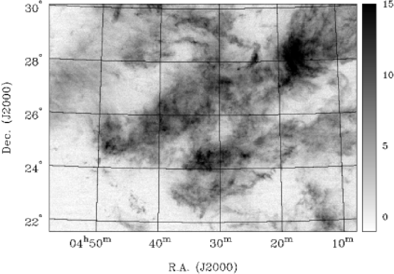
Figure 1: An image of ¹²CO J=1-0 integrated emission from the Taurus Molecular Cloud observed with the Five College Radio Astronomy Observatory 14m telescope and SEQUOIA focal plane array. The high spatial dynamic range reveals varying textures across the cloud and clues to the prevailing physical processes.

2 Velocity Structure Function

A primary goal in the study of ISM physics is to determine the degree of spatial correlation of velocities from observational data. The velocity structure function, $S_{q}(\tau$), defined as

$$S_{q}(\tau)=<|v(r)-v(r+\tau)|^{q}>$$

provides a statistical measure of the q^th order of velocity differences of a field as a function of spatial displacement or lag, $\tau$. For q=2, $S_{2}(\tau)$, the autocorrelation function, $C(\tau)$, and the power spectrum are equivalent statistical measures of the velocity field. $S_{2}(\tau)$ is related to the autocorrelation function as

$$S_{2}(\tau)=2(C(0)-C(\tau))$$

and $C(\tau)$ is the Fourier transform of the power spectrum.

Within the inertial range of a gas flow, the structure function is expected to vary as a power law with spatial lag,

$$S_{q}(\tau)={\delta}v^{q}(\tau)\propto\tau^{\zeta_{q}}.$$

Taking the q^th root of the structure function, this expression can be recast into an equivalent linear form, $(S_{q}(\tau))^{1/q}=<{\delta}v>_{q}=v_{\circ}\tau^{\gamma_{q}}$ where $\gamma_{q}=\zeta_{q}/q$. The power law index, $\gamma_{q}$, measures the degree of spatial correlation and is predicted by model descriptions of turbulence (ex. $\gamma_{3}$=1/3 for Kolmogorov flow). The normalization, $v_{\circ}$, is the amplitude of velocity fluctuations at a fixed scale and offers a convenient measure of the energy density of a flow.

While the expression for the structure function of a velocity field appears straightforward, the construction of $S(\tau)$ from observational data is, in fact, quite challenging. Observers do not measure velocity fields, $v(r)$. Rather, the basic unit of data is a spectrum of line emission that represents a convolution and line of sight integration of density, velocity, and temperature. Furthermore, the effects of chemistry, opacity, and noise can mask or hide contributions to the line profile from features along the line of sight. Despite these limitations, there have been several demonstrated methods to recover the spatial statistics of GMC velocity fields from spectroscopic imaging data.
Analysis of Velocity Centroids: A spectroscopic data cube can be condensed into a 2 dimensional image of centroid velocities determined from the set of line profiles. The spatial statistics of velocity centroids can be formally related to those of the 3 dimensional velocity field (see Ossenkopf etal 2006). With the centroid velocity image, one can assess the power spectrum and hence structure function directly or apply a kernel to calculate the variance of centroid velocities over varying scales (Ossenkopf etal 2006). This method works best under uniform density conditions (Brunt & Mac Low 2004) or with an iterative scheme to account for density fluctuations within the measured power of the observed signal.
Velocity Channel Analysis: Lazarian & Pogosyan (2000) demonstrate a relationship between the power spectra of measured line emission and the respective spectra of the density and velocity fields. The relationship depends on the width of the velocity interval. By calculating the power spectra for both thick and thin velocity windows, one can estimate the power law indices for both the density and velocity fields.
Principal Component Analysis: The spectroscopic data cube is re-ordered onto a set of eigenvectors and eigenimages (Heyer & Schloerb 1997; Brunt & Heyer 2002). The eigenvectors describe the velocity differences in line profiles and the eigenimages convey where those differences occur on the sky. The structure function is constructed from the velocity and angular scales determined from the set of respective eigenvectors and eigenimages that are significant with respect to the noise of the data. To date, the results from PCA have been empirically linked to the velocity structure function parameters based on models under a broad range of physical and observational conditions (Brunt & Heyer 2002; Brunt etal 2003).

2.1 Universality of Turbulence

The three methods described in the previous section provide valuable tools to determine the velocity structure function for a singular interstellar cloud from a set of spectroscopic imaging data. However, for most observations, the statistical and systematic errors for the derived power law index for a given cloud is large ($\sigma_{\gamma}/\gamma\sim$ 10-20%) and preclude a designation of a turbulent flow type. Moreover, given the broad diversity of environments and physical conditions within the molecular ISM, any single measurement of a cloud is unlikely to characterize the complete population. Therefore, it is imperative to analyze a large sample of molecular clouds to assess the impact of local effects and to identify trends and differences.

For Velocity Centroid Analysis, Miesch & Bally (1994) analyzed a set of 12 clouds or sub-regions within giant molecular clouds. They determine a mean value of $\gamma$ to be 0.43$\pm$0.15. Using PCA, Heyer & Brunt (2004) studied 28 clouds in the Perseus and local spiral arms and found $\gamma$=0.49$\pm$0.15. This mean value for $\gamma$ is consistent with highly supersonic turbulence in which the velocity field is characterized by ubiquitous shocks from converging gas streams. The observed distribution of $\gamma$ would exclude a Kolmogorov description of incompressible turbulence unless the velocity fields are characterized by strong intermittency. Moreover, they identified the surprising result that the scaling coefficient, $v_{\circ}$, exhibits little variation from cloud to cloud, despite the large range in cloud sizes and star formation activity. Effectively, when the individual structure functions are overlayed onto a single plot, they form a nearly co-linear set of points (see Figure 2).

Figure 2: The velocity structure functions for 29 clouds derived from PCA of ¹²CO J=1-0 data cubes (Heyer & Brunt 2004). The nearly co-linear set of points attest to the near-invariant functional form of structure functions despite the large range in size and star formation activity. The filled circles are the upper endpoints for each structure function and are equivalent to the size and global line-width for each cloud.

A necessary consequence of this universality is the Larson (1981) cloud-to-cloud size-linewidth relationship. Basically, the upper endpoint of each individual structure function corresponds to the global size and line width of a cloud (filled points in Figure 2). This set of endpoints are correlated only by the fact that the individual velocity structure functions are described by similar values for $\gamma$ and $v_{\circ}$. If there were significant variations of these parameters, then the scatter of points on the cloud-to-cloud relationship would be much larger than is observed. Using Monte Carlo simulations to model the scatter of line-width and size for GMCs in the inner Galaxy, Heyer & Brunt (2004) constrain the variation of $\gamma$ and $v_{\circ}$ to be less than 10-15%.

3 Turbulent Driving Scales

The measurements of velocity structure functions in the molecular ISM point to supersonic turbulent flows in which energy is dissipated in shocks. Unless this energy is replenished within a crossing time, the velocity field would evolve into a Kolmogorov flow comprised exclusively of solenoidal or eddy-like motions. The fact that we observe supersonic turbulence demonstrates that such driving sources must be present in the molecular ISM. Miesch & Bally (1994) summarize candidate sources of energy that could sustain the observed turbulent motions. These include sources that may be resident within the molecular cloud such as protostellar outflows and intermediate and external sources such as HII regions, supernova remnants, and Galactic shear. While all such sources make some contribution, it is important to assess whether any one process is the dominant source.

As first noted by Larson (1981), the universality of velocity structure functions imply a common, external source of energy. Otherwise, those regions with significant localized sources would exhibit significant departures from the observed universal relationship. However, GMCs with rich young clusters, and OB stars show the same amplitude of velocity fluctuations as low mass star forming clouds or even those few clouds with negligible star formation activity (Heyer, Williams, & Brunt 2006). Either there are self-regulating processes independent of energy input scales that maintain this amplitude for most interstellar clouds or such internal energy sources contribute only a small fraction of the energy budget of a molecular cloud.

Large scale driving is also implied by the observation that most of the kinetic energy of a cloud is distributed over the largest scales (Brunt 2003). This is illustrated in Figure 3, which displays the first and second PCA eigenimages derived from ¹²CO J=1-0 emission from the NGC 7538 molecular cloud. The first eigenimage is similar to an integrated intensity image over the full velocity range of the cloud. The second eigenimage exhibits a dipole-like distribution that identifies the large scale shear across the cloud. All clouds studied by Heyer & Brunt (2004) exhibit this dipole distribution in the second eigenimage. For comparison, we show the first two eigenimages calculated from simulated observations of velocity and density fields produced by computational models that are driven at small, intermediate, and large scales. Using the ratio of characteristic scales determined from each eigenimage, one can quantitatively show that the observations are best described by a large scale driving force (Brunt 2003). Protostellar outflows can have a significant but localized impact on a sub-volume of a cloud and can redistributed energy and momentum to large scales (see Bally in these proceedings). However, it seems quite unlikely that an ensemble of widely distributed outflows within the cloud’s volume, can generate the large scale shear that is observed within all molecular clouds analyzed to date.

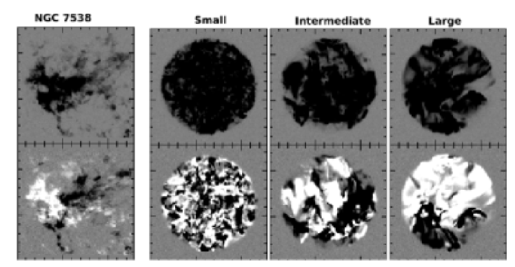
Figure 3: The first two eigenimages derived from ¹²CO J=1-0 emission from the NGC 7538 molecular cloud and model spectra from computation simulations driven at small, intermediate, and large scales (Mac Low 1999). Most observations of molecular clouds exhibit a dipole distribution in the second eigenimage that places most of the kinetic energy within the largest scales of a cloud. The observations are more congruent with computational simulations driven at scales larger than or equal to the size of the cloud.

4 Conclusions

Our understanding of turbulence in the molecular interstellar medium has greatly advanced over the last 10 years owing to more sophisticated computational simulations and ever improving observations. However, there are more critical questions to address to improve these descriptions of turbulence and the role it plays in the star formation process.

• Does the shape of the velocity structure function for a given region change at spatial scales smaller than current resolution limits?

• Does the universality of velocity structure functions extend to the extreme environment of the Galactic Center?

• Are velocity fields of interstellar clouds anisotropic as predicted by the theory of strong, MHD turbulence (Goldreich & Sridhar 1995)?

New telescopes, instrumentation, and analysis methods will be required to address these questions. ALMA will provide both sensitivity and angular resolution to investigate velocity structure functions at the smallest scales and for distant GMCs. The Large Millimeter Telescope will offer the capability to study the low surface brightness component of the molecular ISM to trace the transition from turbulent diffuse material to the dense proto-stellar and proto-cluster cores. These instruments, and others, offer exciting, scientific opportunities to advance our knowledge of interstellar turbulence.