Theory of current instability experiments in magnetic Taylor-Couette flows

Abstract

We consider the linear stability of dissipative MHD Taylor-Couette flow with imposed toroidal magnetic fields. The inner and outer cylinders can be either insulating or conducting; the inner one rotates, the outer one is stationary. The magnetic Prandtl number can be as small as $10^{-5}$, approaching realistic liquid-metal values. The magnetic field destabilizes the flow, except for radial profiles of $B_{\phi}(R)$ close to the current-free solution. The profile with $B_{\rm in}=B_{\rm out}$ (the most uniform field) is considered in detail. For weak fields the TC-flow is stabilized, until for moderately strong fields the $m=1$ azimuthal mode dramatically destabilizes the flow again. There is thus a maximum value for the critical Reynolds number. For sufficiently strong fields (as measured by the Hartmann number) the toroidal field is always unstable, even for $\rm Re=0$.

The electric currents needed to generate the required toroidal fields in laboratory experiments are a few kA if liquid sodium is used, somewhat more if gallium is used. Weaker currents are needed for wider gaps, so a wide-gap apparatus could succeed even with gallium. The critical Reynolds numbers are only somewhat larger than the nonmagnetic values, so such an experiment would require only modest rotation rates.

I Motivation

Taylor-Couette flows of electrically conducting fluid between rotating concentric cylinders are a classical problem of hydrodynamic and hydromagnetic stability theory. It is becoming increasingly clear that the stability of differential rotation combined with magnetic fields is also one of the key problems in MHD astrophysics. For uniform axial magnetic fields this phenomenon is called the magnetorotational instability (MRI). The Keplerian rotation of accretion disks with weak vertical magnetic fields becomes unstable, so that angular momentum is transported outward (star formation) and gravitational energy is efficiently transformed into heat and radiation (quasars). Galactic rotation profiles (approximately $\Omega\propto 1/R$) may also be MRI-unstable, resulting in interstellar MHD turbulence SB99 ; DER04 .

Due to the small size of laboratory experiments, and the extremely small magnetic Prandtl numbers of liquid metals, it is very difficult to achieve the MRI in the lab with a purely axial magnetic field. However, by adding a toroidal field $B_{\phi}\propto 1/R$ (which is current-free within the fluid), it was possible to obtain the MRI experimentally S06 ; R06 , with the most unstable mode being axisymmetric and oscillatory, just as predicted theoretically H05 .

If the field strength is sufficiently great, such a current-free toroidal field yields a magnetorotational instability even without an axial field; the instability is simply non-axisymmetric rather than axisymmetric. The simultaneous occurrence of a stable differential rotation and a stable toroidal field may therefore nevertheless be unstable, provided that the magnetic Reynolds number exceeds $O(100)$ H06 .

In contrast to these magnetorotational instabilities, in which the magnetic field acts as a catalyst, but not as a source of energy, toroidal fields that are not current-free may become unstable more directly, by so-called current or Tayler instabilities T73 ; S99 . Because the source of energy is now the current rather than the differential rotation, these (non-axisymmetric) instabilities can exist even without any differential rotation, provided only the current is large enough. The magnitude depends quite strongly on the precise radial profile of the associated magnetic field $B_{\phi}(R)$, but not on the magnetic Prandtl number. The topic of this paper is how Tayler instabilities interact with differential rotation, and whether it might be possible to realize some of the resulting modes in laboratory experiments. The combination of Tayler instabilities and differential rotation may also be relevant to a broad range of astrophysical problems, including the stability of the solar tachocline, the existence of active solar longitudes KS02 , the flip-flop phenomenon of stellar activity K01 , A-star magnetism BN06 , and even the possibility of ‘a differential rotation driven dynamo in a stably stratified star’ B06 .

II Equations

According to the Rayleigh criterion an ideal flow is stable against axisymmetric perturbations whenever the specific angular momentum increases outwards

$$\frac{{\rm{d}}}{{\rm{d}}R}(R^{2}\Omega)^{2}>0,$$ (1)

where ($R$, $\phi$, $z$) are cylindrical coordinates, and $\Omega$ is the angular velocity. The necessary and sufficient condition for the axisymmetric stability of an ideal Taylor-Couette flow with an imposed azimuthal magnetic field $B_{\phi}$ is

$$\frac{1}{R^{3}}\frac{{\rm{d}}}{{\rm{d}}R}(R^{2}\Omega)^{2}-\frac{R}{\mu_{0}\rho}\frac{{\rm{d}}}{{\rm{d}}R}\left(\frac{B_{\phi}}{R}\right)^{2}>0,$$ (2)

where $\mu_{0}$ is the permeability and $\rho$ the density M54 ; C61 . In particular, all ideal flows can thus be destabilized, by azimuthal magnetic fields with the right profiles and amplitudes. Any fields increasing outward more slowly than $B_{\phi}\propto R$, including in particular the outwardly decreasing current-free field $B_{\phi}\propto 1/R$, have a stabilizing influence though V59 .

Tayler T73 found the necessary and sufficient condition

$$-\frac{{\rm{d}}}{{\rm{d}}R}(RB_{\phi}^{2})>0.$$ (3)

for the non-axisymmetric stability of an ideal fluid at rest. Outwardly increasing fields are therefore unstable now (but $B_{\phi}\propto 1/R$ is still stable). If this condition (3) is violated, the most unstable mode has azimuthal wavenumber $m=1$. In this paper we wish to consider how these Tayler instabilities are modified if the fluid is not at rest, but is instead differentially rotating.

We will find that, depending on the magnitudes of the imposed differential rotation and magnetic fields, and also on the magnetic Prandtl number, a magnetic field may either stabilize or destabilize the differential rotation, and the most unstable mode may be either the axisymmetric Taylor vortex flow, or the non-axisymmetric Tayler instability. We focus on the limit of small magnetic Prandtl numbers appropriate for liquid metals, and calculate the rotation rates and electric currents that would be required to obtain some of these instabilities in liquid metal laboratory experiments.

The governing equations are

$$\frac{\partial\textbf{U}}{\partial t}+(\textbf{U}\nabla)\textbf{U}=-\frac{1}{\rho}\nabla P+\nu\Delta\textbf{U}+\frac{1}{\mu_{0}}{\textrm{curl}}\ \textbf{B}\times\textbf{B},$$ (4)

$$\frac{\partial\textbf{B}}{\partial t}={\textrm{curl}}(\textbf{U}\times\textbf{B})+\eta\Delta\textbf{B},$$ (5)

and

$${\textrm{div}}\ \textbf{U}={\textrm{div}}\ \textbf{B}=0,$$ (6)

where U is the velocity, B the magnetic field, $P$ the pressure, $\nu$ the kinematic viscosity, and $\eta$ the magnetic diffusivity.

The basic state is $U_{R}=U_{z}=B_{R}=B_{z}=0$ and

$$U_{\phi}=R\Omega=a_{\Omega}R+\frac{b_{\Omega}}{R},\qquad B_{\phi}=a_{B}R+\frac{b_{B}}{R},$$ (7)

where $a_{\Omega}$, $b_{\Omega}$, $a_{B}$ and $b_{B}$ are constants defined by

$$a_{\Omega}=\Omega_{\rm{in}}\frac{\hat{\mu}_{\Omega}-{\hat{\eta}}^{2}}{1-{\hat{\eta}}^{2}},\qquad b_{\Omega}=\Omega_{\rm{in}}R_{\rm{in}}^{2}\frac{1-\hat{\mu}_{\Omega}}{1-{\hat{\eta}}^{2}},$$

$$a_{B}=\frac{B_{\rm{in}}}{R_{\rm{in}}}\frac{\hat{\eta}(\hat{\mu}_{B}-\hat{\eta})}{1-\hat{\eta}^{2}},\qquad b_{B}=B_{\rm{in}}R_{\rm{in}}\frac{1-\hat{\mu}_{B}\hat{\eta}}{1-\hat{\eta}^{2}},$$ (8)

where

$$\hat{\eta}=\frac{R_{\rm{in}}}{R_{\rm{out}}},\;\;\;\hat{\mu}_{\Omega}=\frac{\Omega_{\rm{out}}}{\Omega_{\rm{in}}},\;\;\;\hat{\mu}_{B}=\frac{B_{\rm{out}}}{B_{\rm{in}}}.$$ (9)

$R_{\rm{in}}$ and $R_{\rm{out}}$ are the radii of the inner and outer cylinders, $\Omega_{\rm{in}}$ and $\Omega_{\rm{out}}$ are their rotation rates (we will in fact fix $\Omega_{\rm{out}}=0$ for all results presented here), and $B_{\rm{in}}$ and $B_{\rm{out}}$ are the azimuthal magnetic fields at the inner and outer cylinders. The possible magnetic field solutions are plotted in Fig. 1. Note though that – unlike $\Omega$, where $\Omega_{\rm{in}}$ and $\Omega_{\rm{out}}$ are the physically relevant quantities – for $B_{\phi}$ the fundamental quantities are not so much $B_{\rm{in}}$ and $B_{\rm{out}}$, but rather $a_{B}$ and $b_{B}$ themselves. In particular, a field of the form $b_{B}/R$ is generated by running an axial current only through the inner region $R<R_{\rm{in}}$, whereas a field of the form $a_{B}R$ is generated by running an axial current through the entire region $R<R_{\rm{out}}$, including the fluid. One of the aspects we will be interested in later on is how large these currents must be, and whether they could be generated in a laboratory experiment.

We are interested in the linear stability of the basic state (7). The perturbed quantities of the system are given by

$$u_{R},\;R\Omega+u_{\phi},\;u_{z},\;b_{R},\;B_{\phi}+b_{\phi},\;b_{z}.$$ (10)

Applying the usual normal mode analysis, we look for solutions of the linearized equations of the form

$$F=F(R){\rm{exp}}\bigl{(}{\rm{i}}(kz+m\phi+\omega t)\bigr{)}.$$ (11)

The dimensionless numbers of the problem are the magnetic Prandtl number Pm, the Hartmann number Ha, and the Reynolds number Re, given by

$${\rm{Pm}}=\frac{\nu}{\eta},\qquad{\rm{Ha}}=\frac{B_{\rm{in}}R_{0}}{\sqrt{\mu_{0}\rho\nu\eta}},\qquad{\rm{Re}}=\frac{\Omega_{\rm{in}}R_{0}^{2}}{\nu},$$ (12)

where $R_{0}=(R_{\rm{in}}(R_{\rm{out}}-R_{\rm{in}}))^{1/2}$ is the unit of length.

Using (11), linearizing the equations (4) and (5), and representing the result as a system of first order equations, we have

$$\frac{du_{R}}{dR}+\frac{u_{R}}{R}+{\textrm{i}}\frac{m}{R}u_{\phi}+{\textrm{i}}ku_{z}=0,$$

$$\frac{dP}{dR}+{\textrm{i}}\frac{m}{R}X_{2}+{\textrm{i}}kX_{3}+\left(k^{2}+\frac{m^{2}}{R^{2}}\right)u_{R}+$$

$$\qquad\qquad\qquad\qquad+{\textrm{iRe}}(\omega+m\Omega)u_{R}-2\Omega{\textrm{R}e}u_{\phi}-$$

$$\qquad\qquad\qquad\qquad-{\textrm{iHa}}^{2}\frac{m}{R}B_{\phi}b_{R}+2{\textrm{Ha}}^{2}\frac{B_{\phi}}{R}b_{\phi}=0,$$

$$\frac{dX_{2}}{dR}-\left(k^{2}+\frac{m^{2}}{R^{2}}\right)u_{\phi}-{\textrm{iRe}}(\omega+m\Omega)u_{\phi}+$$

$$\qquad\qquad\qquad\qquad+2{\textrm{i}}\frac{m}{R^{2}}u_{R}-\frac{{\textrm{Re}}}{R}\frac{d}{dR}\left(R^{2}\Omega\right)u_{R}+$$

$$+\frac{{\textrm{Ha}}^{2}}{R}\frac{d}{dR}\left(RB_{\phi}\right)b_{R}+{\textrm{iHa}}^{2}\frac{m}{R}B_{\phi}b_{\phi}-{\textrm{i}}\frac{m}{R}P=0,$$

$$\frac{dX_{3}}{dR}+\frac{X_{3}}{R}-\left(k^{2}+\frac{m^{2}}{R^{2}}\right)u_{z}-{\textrm{iRe}}(\omega+m\Omega)u_{z}-$$

$$\qquad\qquad\qquad\qquad\qquad-{\textrm{i}}kP+{\textrm{iHa}}^{2}\frac{m}{R}B_{\phi}b_{z}=0,$$

$$\frac{db_{R}}{dR}+\frac{b_{R}}{R}+{\textrm{i}}\frac{m}{R}b_{\phi}+{\textrm{i}}kb_{z}=0,$$

$$\frac{db_{z}}{dR}-\frac{{\textrm{i}}}{k}\left(k^{2}+\frac{m^{2}}{R^{2}}\right)b_{R}+{\textrm{PmRe}}\frac{1}{k}(\omega+m\Omega)b_{R}+$$

$$\qquad\qquad\qquad\qquad\qquad+\frac{1}{k}\frac{m}{R}X_{4}-\frac{1}{k}\frac{m}{R}B_{\phi}u_{R}=0,$$

$$\frac{dX_{4}}{dR}-\left(k^{2}+\frac{m^{2}}{R^{2}}\right)b_{\phi}-{\textrm{iPmRe}}(\omega+m\Omega)b_{\phi}+$$ (13)

$$\qquad+{\textrm{i}}\frac{2m}{R^{2}}b_{R}-R\frac{d}{dR}\left(\frac{B_{\phi}}{R}\right)u_{R}+{\textrm{PmRe}}R\frac{d\Omega}{dR}b_{r}+$$

$$\qquad\qquad\qquad\qquad\qquad\qquad+{\textrm{i}}\frac{m}{R}B_{\phi}u_{\phi}=0,$$

where $X_{2}$, $X_{3}$ and $X_{4}$ are defined as

$$X_{2}=\frac{du_{\phi}}{dR}+\frac{u_{\phi}}{R},\ \ \ \ X_{3}=\frac{du_{z}}{dR},\ \ \ \ X_{4}=\frac{db_{\phi}}{dR}+\frac{b_{\phi}}{R}.$$ (14)

Length has been scaled by $R_{0}$, time by $\Omega_{\rm{in}}^{-1}$, the basic state angular velocity by $\Omega_{\rm{in}}$, the perturbation velocity by $\eta/R_{0}$, and the magnetic fields, both basic state and perturbation, by $B_{\rm{in}}$.

An appropriate set of ten boundary conditions is needed to solve the system (13). For the velocity the boundary conditions are always no-slip,

$$u_{R}=u_{\phi}=u_{z}=0.$$ (15)

For the magnetic field the boundary conditions depend on whether the walls are insulators or conductors. For conducting walls the radial component of the field and the tangential components of the current must vanish, yielding

$$db_{\phi}/dR+b_{\phi}/R=b_{R}=0.$$ (16)

These boundary conditions are applied at both $R_{\rm{in}}$ and $R_{\rm{out}}$.

For insulating walls the boundary conditions are somewhat more complicated; matching to interior and exterior potential fields then yields

$$b_{\phi}={m\over kR}b_{z},$$ (17)

$$b_{R}+{{\textrm{i}}b_{z}\over I_{m}(kR)}\left({m\over kR}I_{m}(kR)+I_{m+1}(kR)\right)=0,$$ (18)

at $R=R_{\rm{in}}$, and

$$b_{\phi}={m\over kR}b_{z},$$ (19)

$$b_{R}+{{\textrm{i}}b_{z}\over K_{m}(kR)}\left({m\over kR}K_{m}(kR)-K_{m+1}(kR)\right)=0$$ (20)

at $R=R_{\rm{out}}$, where $I_{n}$ and $K_{n}$ are the modified Bessel functions RS02 .

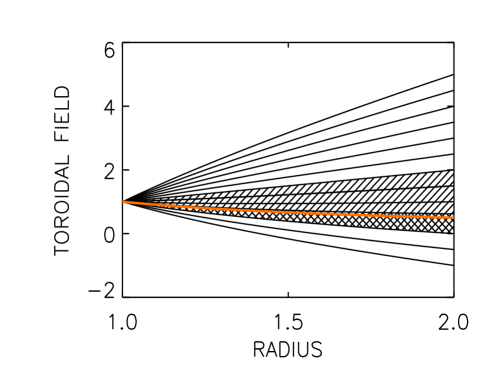
Figure 1: The basic state profiles of $B_{\phi}(R)$, for $\hat{\eta}=0.5$. Remembering that $B_{\phi}(1)$ has been normalized to 1, we find that $\hat{\mu}_{B}$ is given simply by $B_{\phi}(2)$, and can therefore be read off the right-hand axis. The stability domain for $m=1$ (see (21)) is cross-hatched; the cross-hatched and hatched domains together are the stability domain for $m=0$ (see (22)). The current-free solution $B_{\phi}=1/R$ is given by the gray line ($\hat{\mu}_{B}=0.5$). The electric currents inside and outside the inner cylinder are parallel above $\hat{\mu}_{B}=0.5$ and anti-parallel below $\hat{\mu}_{B}=0.5$, that is, the signs of $a_{B}$ and $b_{B}$ are the same above 0.5, and opposite below.

Given the basic state (7), Tayler’s stability condition (3) to nonaxisymmetric perturbations becomes

$$0<\hat{\mu}_{B}<\frac{4\hat{\eta}(1-\hat{\eta}^{2})}{3-2\hat{\eta}^{2}-\hat{\eta}^{4}}\equiv\hat{\mu}_{1}.$$ (21)

Note that $\hat{\mu}_{1}\to 1$ (but is always less than 1) if $\hat{\eta}\to 1$. For $\hat{\eta}=0.5$ we have $\hat{\mu}_{1}=0.62$. Similarly, the stability condition to axisymmetric perturbations becomes

$$0<\hat{\mu}_{B}<\frac{1}{\hat{\eta}}\equiv\hat{\mu}_{0}.$$ (22)

For $\hat{\eta}=0.5$ we have $\hat{\mu}_{0}=2$. For $0<\hat{\eta}<1$ we always have $\hat{\mu}_{1}<\hat{\mu}_{0}$, so that the stability interval (21) for $m=1$ is much smaller than the stability interval (22) for $m=0$, as shown in Fig. 1. The current-free solution $\hat{\mu}_{B}=0.5$ is of course always stable.

III Basic Results

Figure 2: Marginal stability curves for $m=0$ (dashed) and $m=1$ (solid). The hatched area is thus the region that is stable to both. Magnetic Prandtl numbers as indicated on each plot.

Figure 2 shows how the stability curves depend on $\rm Ha$ and $\rm Re$, for $\rm Pm=10$, 1, 0.1 and 0.01, with $\hat{\mu}_{\Omega}=0$ (stationary outer cylinder) and $\hat{\mu}_{B}=1$ ($B_{\phi}$ as uniform as possible). For $\rm Ha=0$ we find that $m=0$ goes unstable before $m=1$, at the critical Reynolds number $\rm Re_{crit}=68$; this is just the familiar value for the onset of nonmagnetic Taylor vortices (at this particular radius ratio). Being entirely nonmagnetic, this value obviously does not depend on $\rm Pm$. At the other limiting case, $\rm Re=0$, we find that only $m=1$ goes unstable, at the critical Hartmann number $\rm Ha_{crit}=150$. These Tayler instabilities also turn out to be independent of $\rm Pm$, despite being driven by the magnetic field.

We are interested in how these two limiting cases $\rm Ha=0$ and $\rm Re=0$ are connected, and how the two types of instabilities interact when neither parameter is zero. The two instabilities certainly are connected; the $m=1$ modes in the two limiting cases are smoothly joined to one another for all Prandtl numbers. The nature of the interaction is quite different though, depending on $\rm Pm$.

Turning to $\rm Pm=1$ first, we see that there is relatively little interaction between rotational and magnetic effects; instability simply sets in as long as either $\rm Ha>Ha_{crit}$ or $\rm Re>Re_{crit}$. For $\rm Pm=10$ the situation is very different. There we find a broad range of parameters, for example $\rm Ha=100$ and $\rm Re=50$, that would be stable if rotational or magnetic effects were acting alone, but which are now unstable, due to the interaction between the two (see also GF97 ). Finally, for $\rm Pm=0.1$ we have the opposite situation, namely a range of parameters, for example $\rm Ha=100$ and $\rm Re=100$, that would be unstable if rotational effects were acting alone, but which are now stable.

Small Pm are generally stabilizing. The opposite is true for $\rm Pm>1$. As shown in Fig. 2 (top) instability then also sets in for Hartmann numbers less than 150. In other words, for Hartmann numbers exceeding around 50, the critical Reynolds number for the onset of instability is much smaller than 68.

IV Liquid metals

Having explored the general behavior for a range of magnetic Prandtl numbers, we now focus attention on the limit of very small Pm, such as would apply for experiments involving liquid metals. We will here consider conducting and insulating boundary conditions separately.

IV.1 Conducting cylinder walls

Figure 3 shows results for various values of $\hat{\mu}_{B}$; $a_{B}$ and $b_{B}$ are the same sign for the values on the left, and the opposite sign for the values on the right. The profile that is closest to being current-free is $\hat{\mu}_{B}=0$, and indeed we find there that even for Ha=200 there is no sign of any destabilizing influence of the field, for either axisymmetric or nonaxisymmetric perturbations. For $0<\hat{\mu}_{B}<\hat{\mu}_{1}$ the magnetic field stabilizes the flow for both $m=0$ and $m=1$.

For $\hat{\mu}_{1}<\hat{\mu}_{B}<\hat{\mu}_{0}$ the $m=1$ mode should be unstable, while the $m=0$ mode should be stable. The values $\hat{\mu}_{B}=1$ and $\hat{\mu}_{B}=2$ are examples of this situation. There is always a crossover point at which the most unstable mode changes from $m=0$ to $m=1$. Note also how for $\hat{\mu}_{B}=1$, the critical Reynolds number increases for the $m=0$ mode, before suddenly decreasing for the $m=1$ mode (Fig. 3, left bottom plot). We have the interesting situation therefore that weak fields initially stabilize the TC-flow, before stronger fields eventually destabilize it, via a non-axisymmetric mode. Beyond $\rm Ha=150$ (the same value we saw previously in Fig. 2), the flow is unstable even for $\rm Re=0$.

Except for the almost current-free profile $\hat{\mu}_{B}=0$, all other values share this feature, that there is a critical Hartmann number beyond which the basic state is unstable even for $\rm Re=0$. Let Ha⁽⁰⁾ and Ha⁽¹⁾ denote these critical Hartmann numbers, for $m=0$ and 1 respectively. For the profiles with the largest gradients both modes are unstable. Strikingly, in these cases $m=0$ is always more unstable than $m=1$, that is, $\rm Ha^{(0)}<Ha^{(1)}$, see the plots for $\hat{\mu}_{B}=4$ and $\hat{\mu}_{B}=-2$ of Fig. 3.

Figure 3: The marginal stability curves for $m=0$ (dashed) and $m=1$ (solid). Pm$=10^{-5}$, $\hat{\eta}=0.5$, $\hat{\mu}_{\Omega}=0$, and $\hat{\mu}_{B}$ as indicated. Note also how the critical Reynolds numbers are always of the same order of magnitude as the nonmagnetic result 68, which is very easy to achieve in the laboratory.

IV.2 The required electric currents

Let $I_{\rm{axis}}$ be the axial current inside the inner cylinder and $I_{\rm{fluid}}$ the axial current through the fluid (i.e. between inner and outer cylinder). The toroidal field amplitudes at the inner and outer cylinders are then

$$B_{\rm{in}}=\frac{I_{\rm{axis}}}{5R_{\rm{in}}},\qquad B_{\rm{out}}=\frac{(I_{\rm{axis}}+I_{\rm{fluid}})}{5R_{\rm{out}}},$$ (23)

where $R$, $B$ and $I$ are measured in cm, Gauss and Ampere. Expressing $I_{\rm{axis}}$ and $I_{\rm{fluid}}$ in terms of our dimensionless parameters one finds

$$I_{\rm{axis}}=5{\rm Ha}\ \frac{\hat{\eta}^{1/2}}{(1-\hat{\eta})^{1/2}}(\mu_{0}\rho\nu\eta)^{1/2}$$ (24)

and

$$I_{\rm{fluid}}=\frac{\hat{\mu}_{B}-\hat{\eta}}{\hat{\eta}}I_{\rm{axis}},$$ (25)

in Ampere. Note also how the required currents depend on the radius ratio $\hat{\eta}$, but not on the actual physical dimensions $R_{\rm{in}}$ and $R_{\rm{out}}$. Making the entire device bigger thus reduces the current density, inversely proportional to the square of the size. By making the device sufficiently large one can thereby prevent Ohmic heating within the fluid from becoming excessive.

Table 1: Material parameters of liquid metals that might be used for magnetic TC-experiments.

	$\rho$ [g/cm3]	$\nu$ [cm2/s]	$\eta$ [cm2/s]	$\sqrt{\mu_{0}\rho\nu\eta}$
sodium	0.92	$7.10\cdot 10^{-3}$	$0.81\cdot 10^{3}$	8.15
gallium-indium-tin	6.36	$3.40\cdot 10^{-3}$	$2.43\cdot 10^{3}$	25.7

The results for the critical Hartmann numbers are now applied to two different conducting liquid metals, sodium and gallium-indium-tin S06 , whose material parameters are given in Table 1. We also wish to consider the effect of varying the radius ratio $\hat{\eta}$. Tables 2–4 give the values of the electric currents needed to reach the lesser of Ha⁽⁰⁾ and Ha⁽¹⁾, for the three values $\hat{\eta}=0.25$, 0.5 and 0.75, and for $\hat{\mu}_{B}$ ranging from $-10$ to 10 in each case. Note that for large $|\hat{\mu}_{B}|$, Ha⁽⁰⁾ scales as 1/$\hat{\mu}_{B}$, and $I_{\rm{fluid}}$ approaches a constant value. The calculated currents are lower for fluids with smaller $\sqrt{\mu_{0}\rho\nu\eta}$ (i.e. sodium is better than gallium).

In these Tables, the most interesting experiment, with the almost uniform field $\hat{\mu}_{B}=1$ (see Fig. 3, top-right) is indicated in bold. For a container with a medium gap of $\hat{\eta}=0.5$, parallel currents along the axis and through the fluid of 6.16 kA for sodium and 19.4 kA for gallium are necessary. Such sodium experiments should indeed be possible. Experiments with a wider $\hat{\eta}=0.25$ gap are even easier; in that case even gallium experiments should be possible, with a current of 9.29 kA required (see Table 2).

The Reynolds numbers that would be required to obtain not just these $\rm Re=0$ pure Tayler instabilities, but also the transition points from $m=0$ to $m=1$ are also not difficult to achieve; for $R_{\rm{out}}\sim 10$ cm, say, rotation rates of order $10^{-2}$ Hz are already enough.

Table 2: Characteristic Hartmann numbers and electric currents for a wide gap container ($\hat{\eta}=0.25$) with conducting walls, using either sodium or gallium-indium-tin (in brackets).

$\hat{\mu}_{B}$	Ha(0)	Ha(1)	$I_{\rm{axis}}$ [kA]	$I_{\rm{fluid}}$ [kA]
-10	2.29	2.05	0.0483 (0.152)	-1.98 (-6.24)
-5	4.23	3.98	0.0937 (0.296)	-1.97 (-6.21)
-4	5.14	4.93	0.116 (0.366)	-1.97 (-6.22)
-3	6.63	6.50	0.153 (0.483)	-1.99 (-6.27)
-2	9.69	9.71	0.228 (0.721)	-2.05 (-6.49)
-1	24.7	22.5	0.530 (1.67)	-2.65 (-8.35)
1	$\infty$	41.7	0.982 (3.10)	2.94 (9.29)
2	$\infty$	13.8	0.325 (1.02)	2.27 (7.17)
3	$\infty$	8.27	0.195 (0.614)	2.14 (6.75)
4	$\infty$	5.93	0.140 (0.440)	2.09 (6.60)
5	10.8	4.63	0.109 (0.344)	2.07 (6.53)
10	3.23	2.205	0.0519 (0.164)	2.02 (6.39)

Table 3: The same as in Table 2 but for $\hat{\eta}=0.5$

$\hat{\mu}_{B}$	Ha(0)	Ha(1)	$I_{\rm{axis}}$ [kA]	$I_{\rm{fluid}}$ [kA]
-10	3.96	5.02	0.161 (0.509)	-3.39 (-10.7)
-5	7.73	9.85	0.315 (0.994)	-3.47 (-10.9)
-4	9.61	12	0.392 (1.24)	-3.53 (-11.1)
-3	12.8	16.2	0.522 (1.65)	-3.65 (-11.5)
-2	19.8	24.8	0.807 (2.55)	-4.04 (-12.7)
-1	59.3	63.7	2.42 (7.63)	-7.25 (-22.9)
1	$\infty$	151	6.16 (19.4)	6.16 (19.4)
2	$\infty$	35.3	1.44 (4.54)	4.32 (13.6)
3	21.0	20.6	0.840 (2.65)	4.20 (13.2)
4	13.2	14.6	0.538 (1.70)	3.77 (11.9)
5	9.84	11.4	0.401 (1.27)	3.61 (11.4)
10	4.44	5.4	0.181 (0.571)	3.44 (10.8)

Table 4: The same as in Table 2 but for $\hat{\eta}=0.75$ (narrow gap container).

$\hat{\mu}_{B}$	Ha(0)	Ha(1)	$I_{\rm{axis}}$ [kA]	$I_{\rm{fluid}}$ [kA]
-10	9.27	12.2	0.655 (2.06)	-9.39 (-29.6)
-5	18.6	24.1	1.31 (4.13)	-10.0 (-31.5)
-4	23.3	30.1	1.65 (5.20)	-10.5 (-33.1)
-3	31.6	40.3	2.23 (7.03)	-11.1 (-35.0)
-2	50.4	63.4	3.56 (11.2)	-13.1 (-41.3)
-1	163.	177.	11.5 (36.3)	-26.8 (-84.5)
1	$\infty$	632	44.6 (141)	14.9 (47.0)
2	66.8	87.3	4.72 (14.9)	7.87 (24.8)
3	36.5	49.8	2.58 (8.14)	7.74 (24.4)
4	25.8	35.2	1.82 (7.89)	5.74 (24.9)
5	20.1	27.3	1.42 (4.48)	8.05 (25.4)
10	9.63	13.0	0.680 (2.14)	8.39 (26.5)

IV.3 Insulating cylinder walls

Table 5: The same as in Table 2 (wide gap, $\hat{\eta}=0.25$) but for insulating cylinders.

$\hat{\mu}_{B}$	Ha0	Ha1	$I_{\rm{axis}}$ [kA]	$I_{\rm{fluid}}$ [kA]
-10	3.63	1.79	0.0421 (0.133)	-1.73 (-5.45)
-5	6.65	3.55	0.0836 (0.264)	-1.76 (-5.54)
-4	8.04	4.42	0.104 (0.328)	-1.77 (-5.58)
-3	10.3	5.89	0.139 (0.437)	-1.81 (-5.68)
-2	14.7	8.91	0.210 (0.662)	-1.89 (-5.60)
-1	30.6	20.5	0.483 (1.52)	-2.42 (-7.60)
1	$\infty$	30.7	0.723 (2.28)	2.17 (6.84)
2	$\infty$	10.7	0.252 (0.794)	1.76 (5.56)
3	$\infty$	6.63	0.156 (0.492)	1.72 (5.41)
4	$\infty$	4.83	0.114 (0.359)	1.71 (5.39)
5	17.4	3.81	0.0897 (0.283)	1.70 (5.38)
10	5.18	1.86	0.0438 (0.138)	1.71 (5.38)

Table 6: The same as in Table 3 (medium gap, $\hat{\eta}=0.5$) but for insulating cylinders.

$\hat{\mu}_{B}$	Ha0	Ha1	$I_{\rm{axis}}$ [kA]	$I_{\rm{fluid}}$ [kA]
-10	6.09	4.66	0.190 (0.599)	-3.99 (-12.6)
-5	11.8	9.31	0.380( 1.20)	-4.18 (-13.2)
-4	14.6	11.7	0.477 (1.50)	-4.29 (-13.5)
-3	19.4	15.7	0.640 (2.02)	-4.48 (-14.1)
-2	29.3	25.2	1.03 (3.24)	-5.15 (-16.2)
-1	73.6	64.6	2.63 (8.31)	-7.89 (-24.9)
1	$\infty$	109.	4.44 (14.0)	4.44 (14.0)
2	$\infty$	28.1	1.15 (3.61)	3.45 (10.8)
3	32.6	17.2	0.701 (2.21)	3.51 (11.1)
4	20.5	12.5	0.510 (1.61)	3.57 (11.3)
5	15.3	9.81	0.400 (1.26)	3.60 (11.3)
10	6.86	4.78	0.195 (0.615)	3.71 (11.7)

Table 7: The same as in Table 4 (narrow gap, $\hat{\eta}=0.75$) but for insulating cylinders.

$\hat{\mu}_{B}$	Ha0	Ha1	$I_{\rm{axis}}$ [kA]	$I_{\rm{fluid}}$ [kA]
-10	14.2	13.8	0.975 (3.07)	-14.0 (-44.0)
-5	28.2	27.7	1.96 (6.17)	-15.0 (-47.3)
-4	35.4	34.9	2.46 (7.77)	-15.6 (-49.2)
-3	47.7	47.2	3.33 (10.5)	-16.7 (-52.5)
-2	74.8	74.7	5.28 (16.6)	-19.4 (-60.9)
-1	208.	205.	14.5 (45.7)	-33.8 (-107)
1	$\infty$	464.	32.8 (103.)	10.9 (34.3)
2	103.	80.3	5.67 (17.9)	9.45 (29.8)
3	56.2	49.1	3.47 (10.9)	10.4 (32.7)
4	39.7	35.9	2.54 (7.99)	11.0 (34.6)
5	30.9	28.4	2.18 (6.32)	12.4 (35.8)
10	14.8	13.9	0.982 (3.10)	12.1 (38.2)

Figure 4: The same as in Fig. 3 but for insulating cylinder walls.

Calculations were also done for insulating cylinder walls; the results are given in Fig. 4. They are generally similar as those for the conducting cylinders, but with one important exception. The $m=0$ and $m=1$ stability curves now almost always cross each other, as they do for conducting cylinders only for almost current-free $B_{\phi}$ profiles. One can again observe for not too steep profiles (for $\hat{\mu}_{B}\simeq\pm 1$) how for weak fields the $m=0$ mode stabilizes the rotation until beyond the cross-over point the $m=1$ mode strongly destabilizes the rotation.

V Conclusions

We have shown how complex the interaction of magnetic fields and differential rotation can be in Taylor-Couette flows, including also a strong dependence on the magnetic Prandtl number. For large Pm the field destabilizes the differential rotation, whereas for small Pm it stabilizes it. However, if the field (or rather the current) is too great, then the Tayler instabilities will always destabilize any differential rotation.

In order to prepare laboratory experiments, we also did calculations at values of Pm appropriate for liquid metals, for both conducting and insulating cylinder walls. In particular, we considered the almost uniform field profile $\hat{\mu}_{B}=1$. For both conducting and insulating boundaries, the field is initially stabilizing, but after the most unstable mode switches from $m=0$ to $m=1$ it is strongly destabilizing, until the pure Tayler instability sets in even at $\rm Re=0$.

For various gap widths and field profiles, we also computed the critical Hartmann numbers and the corresponding electric currents. Tables II–VII give the required currents for both conducting and insulating walls; note how insulating walls (Tables V–VII) typically require lower currents than conducting walls (Tables II–IV). The other clear trend is that the currents are lesser for wider gaps and greater for narrower gaps. An optimal experiment might therefore have $\hat{\eta}=0.25$, insulating walls, and $\hat{\mu}_{B}=1$, which would require only 6.84 kA even with gallium-indium-tin (Table V).

- (1) J. A. Sellwood and S. A. Balbus, Astrophys. J. 511, 660 (1999).
- (2) N. Dziourkevitch, D. Elstner, and G. Rüdiger, Astron. Astrophys. 423, L29 (2004).
- (3) F. Stefani, T. Gundrum, G. Gerbeth, G. Rüdiger, M. Schultz, J. Szklarski, and R. Hollerbach, Phys. Rev. Lett. 97, 184502 (2006).
- (4) G. Rüdiger, R. Hollerbach, F. Stefani, T. Gundrum, G. Gerbeth, and R. Rosner, Astrophys. J. 649, L145 (2006).
- (5) R. Hollerbach and G. Rüdiger, Phys. Rev. Lett. 95, 124501 (2005).
- (6) R. Hollerbach, G. Rüdiger, M. Schultz and D. Elstner, Phys. Rev. Lett. (submitted).
- (7) R. J. Tayler, Mon. Not. R. Astron. Soc. 161, 365 (1973).
- (8) H. C. Spruit, Astron. Astrophys. 349, 189 (1999).
- (9) N. A. Krivova and S. K. Solanki, Astron. Astrophys. 394, 701 (2002).
- (10) H. Korhonen, S. V. Berdyugina, K. G. Strassmeier, and I. Tuominen, Astron. Astrophys. 379, L30 (2001).
- (11) J. Braithwaite and Å. Nordlund, Astron. Astrophys. 450, 1077 (2006).
- (12) J. Braithwaite, Astron. Astrophys. 453, 687 (2006).
- (13) D. Michael, Mathematika 1, 45, (1954).
- (14) S. Chandrasekhar, Hydrodynamic and Hydromagnetic Stability (Clarendon, Oxford 1961).
- (15) E. P. Velikhov, Sov. Phys. JETP 9, 995 (1959).
- (16) G. Rüdiger and D. Shalybkov, Phys. Rev. E 66, 016307 (2002).
- (17) P. A. Gilman and P. A. Fox, Astrophys. J. 484, 439 (1997).