Population Synthesis in the Blue IV. Accurate Model Predictions for Lick Indices and UBV Colors in Single Stellar Populations

Abstract

We present a new set of model predictions for 16 Lick absorption line indices from $H\delta$ through Fe5335, and UBV colors for single stellar populations with ages ranging between 1 and 15 Gyr, and [Fe/H] ranging from –1.3 to +0.3, and variable abundance ratios. The models are based on accurate stellar parameters for the Jones library stars and a new set of fitting functions describing the behavior of line indices as a function of effective temperature, surface gravity, and iron abundance. The abundances of several key elements in the library stars have been obtained from the literature in order to characterize the abundance pattern of the stellar library, thus allowing us to produce model predictions for any set of abundance ratios desired. We develop a method to estimate mean ages and abundances of iron, carbon, nitrogen, magnesium and calcium that explores the sensitivity of the various indices modeled to those parameters. The models are compared to high S/N data for Galactic clusters spanning the range of ages, metallicities and abundance pattern of interest. Essentially all line indices are matched when the known cluster parameters are adopted as input. Cluster spectroscopic ages determined from different Balmer line indices are consistent to within $\sim$ 1 Gyr. The models can predict confidently the above elemental abundances to within $\pm$ 0.1 dex and ages to within $\pm$ 1 (0.5) Gyr for old (intermediate-age) stellar populations. Comparing the models to high-quality data for galaxies in the nearby universe, we reproduce previous results regarding the enhancement of light elements and the spread in the mean luminosity-weighted ages of early-type galaxies. When the results from the analysis of blue and red indices are contrasted, we find good consistency in the [Fe/H] that is inferred from different Fe indices. Applying our method to stacked SDSS spectra of early-type galaxies brighter than $L^{\star}$, we find mean luminosity-weighted ages of the order of $\sim$ 8 Gyr and iron abundances slightly below solar. Abundance ratios, [X/Fe], tend to be higher than solar, and are positively correlated with galaxy luminosity. Of all elements, nitrogen is the more strongly correlated with galaxy luminosity, which seems to indicate secondary nitrogen enrichment. If that interpretation is correct, this result may impose a lower limit of 50-200 Myr to the timescale of star formation in early-type galaxies. Unlike clusters, galaxies show a systematic effect whereby higher-order, bluer, Balmer lines yield younger ages than $H\beta$. This age discrepancy is stronger for lower luminosity galaxies. We examine four possible scenarios to explain this trend. Contamination of the bluer indices by a metal-poor stellar population with a blue horizontal branch cannot account for the data. Blue stragglers and abundance-ratio effects cannot be ruled out, as they can potentially satisfy the data, even though this can only be achieved by resorting to extreme conditions, such as extremely high [O/Fe] or specific blue-straggler frequencies. The most likely explanation is the presence of small amounts of a young/intermediate-age stellar population component. We simulate this effect by producing two-component models and show that they provide a reasonably good match to the data when the mass fraction of the young component is typically a few %. If confirmed, this result implies star formation has been extended in early-type galaxies, and more so in less massive galaxies, which seems to lend support to the “downsizing” scenario. Moreover, it implies that stellar population synthesis models are capable of constraining not only the mean ages of stellar populations in galaxies, but also their age spread.

1. Introduction

With the consolidation of the cold dark matter scenario for structure formation (e.g., Blumenthal et al. 1984), the study of galaxy evolution is entering an era of high precision, such that crucial questions can only be answered on the basis of accurate data and models. For instance, roughly half of all stellar mass in today’s universe inhabits early-type galaxies (Fukugita, Hogan & Peebles 1998) yet a definitive picture of the history of star formation in these systems is still lacking. That is one of the chief motivations for the construction of stellar population synthesis models. High accuracy is required for such models because the spectrophotometric evolution of stellar populations proceeds at a very slow pace after the first Gyr or so, which makes it very hard to extract reliable age information from the integrated light of galaxies when most of the stars are old.

Stellar population synthesis aims at discerning the stellar mix in galaxies from their integrated spectral energy distributions. With that intent, models are computed which predict the evolution of magnitudes, colors, and absorption line indices of stellar populations. Comparisons of these models with the observations should constrain the age and metal abundance distribution of stars in galaxies, thus yielding constraints on their histories of star formation and chemical enrichment. The problem is complicated, however, as the spectral energy distributions of stellar populations respond to variations of different parameters in degenerate ways. One popular example is the age-metallicity degeneracy (e.g., Faber 1972, 1973, O’Connell 1980, Rose 1985, Renzini 1986, Worthey 1994), whereby stellar population colors and most absorption line strengths respond similarly to variations of age and metallicity. Major improvement was brought by the introduction of the Lick/IDS system of equivalent widths (Burstein et al. 1984, Gorgas et al. 1993, Worthey et al. 1994), which systematized the measurements of absorption line strengths in the spectra of stars and galaxies. Later on, with the development of models to predict the strengths of these indices as a function of stellar population parameters (e.g., Worthey et al. 1994, Worthey 1994, Bressan, Chiosi & Fagotto 1994, Weiss, Peletier & Matteucci 1995, Borges et al. 1995), key aspects of the evolution of early-type galaxies were unveiled. Worthey, Faber & González (1992) showed that giant ellipticals are characterized by enhancement of the abundances of light elements (see also Peterson 1976, O’Connell 1980, Peletier 1989), which possibly indicates that the bulk of their stars were formed in a rapid ($\mathrel{\hbox{\raise 2.15277pt\hbox{$<$}\hbox to0.0pt{\hss\lower 2.15277pt\hbox{$\sim$}}}}$ 1 Gyr) star formation event. Later on, Worthey (1994) showed that the $H\beta$ index is more sensitive to age than to metallicity, thus allowing to break the age-metallicity degeneracy. Further extension of the models towards higher-order Balmer lines was accomplished by Worthey & Ottaviani (1997). Despite some controversy as to how clean an age indicator a given Balmer line is, this sparked a world-wide industry to estimate mean-ages and metallicities of stellar populations in galaxies. Until very recently, however, most of the work has been focussed on the “green” Lick indices: $H\beta$, Fe5270, Fe5335, Mg₂, and Mg $b$. The blue indices ($\lambda\mathrel{\hbox{\raise 2.15277pt\hbox{$<$}\hbox to0.0pt{\hss\lower 2.15277pt\hbox{$\sim$}}}}4500{\rm\AA}$) were for a while relegated to a relative ostracism due to problems in the calibration of original Lick/IDS data in the blue and to intrinsic modeling difficulties related to the higher crowding of lines in that spectral region, which renders a clean absorption line strength measurement extremely difficult.

But the integrated spectra of early-type galaxies in the blue contain a wealth of information for those who take the challenge, as demonstrated by the pioneering work of Rose (1985, 1994). Moreover, combining accurate models in the blue to those currently available for red indices adds the benefit of a wider baseline, which proves to be extremely advantageous for stellar population studies (O’Connell 1976). Another important benefit of constructing consistent models within a large baseline that includes the blue spectral region lies in the need to interpret the integrated spectra of remote galaxies. Ongoing surveys based on 8-10 m class telescopes are obtaining large amounts of high-quality spectroscopic data for galaxies at z $\sim$ 1 (e.g., DEEP survey, Davis et al. 2003; VIRMOS-VLT Deep Survey, Le Févre et al. 2001, K20, Cimatti et al. 2002, Gemini Deep Deep Survey, Abraham et al. 2004). Because of strong telluric emission lines in the far red/near infrared, only the blue spectral region is accessible from the ground for galaxies at the involved redshifts, using current instrumental capabilities. Therefore, models which are consistent from the blue to the red are crucial, so that the mean ages and metallicities of remote systems, which are necessarily based on blue spectra, can be safely tied to those measured in nearby galaxies.

In this paper, we present a new set of model predictions for line indices and UBV colors of single stellar populations. Our goal is to produce models that are accurate and consistent throughout the spectral range going from $\lambda\lambda$ 4000 to 5400 ${\rm\AA}$. This is the fourth paper of a series dedicated to the study of stellar populations in the optical, with emphasis in the blue spectral region. In Schiavon et al. (2002a,b, hereafter Papers I and II), we studied the integrated spectrum of the moderately metal-rich Galactic globular cluster 47 Tuc and in Schiavon, Caldwell & Rose (2004, hereafter Paper III) we constructed and analyzed the integrated spectrum of the metal-rich, intermediate-age Galactic open cluster, M 67.

Our models are based on a new set of fitting functions for indices in the Lick system. We omit on purpose the “IDS” part of the usual nomenclature of this system of equivalent widths because, as it will be seen in Section 2.2, our models are not in the Lick/IDS system, as they are not based on index measurements taken in the standard Lick/IDS stellar library (Burstein et al. 1984, Gorgas et al. 1993, Worthey et al. 1994). Instead, the index measurements that form the backbone of our models were taken in a much more recent spectral library, by Jones (1999). The spectra from that library are flux-calibrated, thus being unaffected by the response curve of the old Lick Image Dissector Scanner. However, for reasons that will become clear in Section 2.2, our line indices are measured at the relatively low resolution of the original Lick/IDS system. We are aware of the ongoing work on the construction of better spectral libraries with higher resolution than that of the Lick system, and spanning a wide range of stellar parameters (e.g., Le Borgne et al. 2003, Valdes et al. 2004). However, when this project started, these libraries were not available publicly. Moreover, our main goal is to apply these models to study distant giant early-type galaxies, whose spectra are irretrievably smoothed by their high velocity dispersions to resolutions that are comparable to that of the Lick system ($\sim$ 8 ${\rm\AA}$).

It is also important to justify here our reasons to adopt fitting functions, even though in Papers I and II we produced synthetic spectra of single stellar populations. The main reason is that the degree of accuracy needed for such model predictions cannot be achieved on the basis of the Jones (1999) library, because of its relatively limited coverage of stellar parameter space. Moreover, fitting functions are very convenient for a number of reasons. For instance, they can be easily implemented in any evolutionary synthesis code. In addition, models based on fitting functions can also be corrected to yield line index predictions for varying abundance patterns.

A key feature of our models is related to the stellar parameters adopted for the library stars. They have to be homogeneous, internally accurate, and free of important systematic effects. Accuracy is very important, for it allows a precise assessment of the behavior of stellar observables as a function of fundamental parameters. This aspect of our models was very carefully crafted.

One of the chief applications of stellar population synthesis is the estimation of mean elemental abundances of stars in remote systems from absorption line indices measured in their integrated spectra. Ratios of elemental abundances, such as that between magnesium and iron, hold important clues for the history of star formation and chemical evolution of galaxies (e.g., Matteucci & Tornambè 1987; Wheeler, Sneden & Truran 1989; Peletier 1989, Worthey, Faber & González 1992; Edvardsson et al. 1993; McWilliam 1997; Worthey 1998). Therefore, models that are able to convert, for instance, Mg $b$ and Fe4383 measurements into a mean [Mg/Fe] for a given galaxy are highly desirable.

This is unfortunately not very easy to achieve because of two reasons. First, the integrated spectra of galaxies are smoothed due to the intrinsic dispersion of the velocities of their member stars along the line of sight. As a result, all the absorption lines are blended, making it impossible to isolate absorption features that cleanly indicate the abundance of a given chemical species. Second, detailed abundance patterns for the majority of the stars used in the construction of the models—hence the abundance pattern of the models themselves—are unknown.

A method to address these difficulties was devised by Trager et al. (2000) and further developed by Proctor & Sansom (2002), Thomas, Maraston & Bender (2003a), and Thomas, Maraston & Korn (2004), and Korn, Maraston & Thomas (2005). The core of this method resides in the use of sensitivities of Lick indices to variations in the elemental abundances of all the relevant chemical species with absorption lines included in each index passband and pseudo-continuum windows. Trager et al. used the Tripicco & Bell (1995) tabulations of index sensitivities computed from spectrum synthesis adopting model atmospheres of stars with representative stellar parameters. The sensitivities were used to integrate the effect of abundance ratio variations of the main Lick indices in the green region. That allowed them to estimate by how much the mean [Mg/Fe] of the stellar populations of elliptical galaxies in their sample depart from that of the spectral library used as input in their models (which they assumed to be equal to solar). The method was extended by Thomas et al. (2003a) to include all the Lick/IDS indices in Worthey et al. (1994). Later on, Korn et al. (2005) computed new sensitivities that include also the higher order Balmer lines defined by Worthey & Ottaviani (1997).

It is vital for the success of this method that the abundance pattern of the models be well-known. As emphasized by Thomas et al. (2003a), models that are based on empirical stellar libraries are characterized by an abundance pattern that is equal to that of the stars that make up the adopted spectral library. Therefore, we decided to survey the literature for elemental abundance determinations of the stars in the spectral library adopted in our models. We provide mean abundance ratios as a function of [Fe/H] for several important chemical elements. This information is used in Section 4.3, in combination with our fitting functions and the Korn et al. (2005) sensitivity tables, to produce model predictions for varying abundance patterns. We present a detailed study of the response of line indices to age and elemental abundance variations, in order to explore ways in which our models can be used to constrain those parameters for intermediate-age and old stellar populations. On the basis of the insights gained in this study, we develop a new method to estimate the mean luminosity-weighted age of stellar populations, as well as their abundances of iron, magnesium, calcium, carbon, and nitrogen.

In a degenerate problem like that of stellar population synthesis, knowing the answers that are to be expected for a given set of input parameters is priceless. Therefore, a detailed comparison of our model predictions for single stellar populations with accurate data for well-known Galactic clusters is performed. Our goal is to match all 16 indices for a small sample of clusters which spans the entire range of stellar population parameters of interest. We hope to convince the reader that significant advance has been made towards meeting this initial goal. At the end of this exercise, we show that the ages and metal abundances derived from application of our models to the integrated light of stellar populations is meaningful in an absolute sense, i.e., they are consistent with metallicity and age scales defined by known local systems, such as Galactic clusters and stars in the solar neighborhood.

Once we are convinced that the comparison of the models with cluster data gives satisfactory results, we turn our attention to galaxies. In this paper, we refrain from pursuing a detailed analysis of the galaxy data and instead make more qualitative comparisons between data and models and discuss what can be learned therefrom. We first compare our models to the data from Trager et al. (2000a,b, henceforth simply Trager et al. 2000) in order to make sure that we reproduce some well established results, such as the $\alpha$-enhancement characteristic of massive early-type galaxies and the spread in the mean ages of their stellar populations. Next, we take advantage of the wide baseline covered by our models to compare them to measurements taken on stacked spectra of early-type galaxies from the Sloan Digital Sky Survey (Eisenstein et al. 2003). We determine the mean abundances of iron, magnesium, calcium, and, for the first time, those of carbon and nitrogen for the stars in early-type galaxies. The behavior of these abundances as a function of galaxy luminosity is studied. Of all abundance ratios studied, [N/Fe] is the one that seems to be the most strongly correlated with galaxy luminosity, perhaps indicating an important secondary source of nitrogen enrichment in these galaxies. If confirmed, this result may be telling us that there is a minimum duration for the star formation in early-type galaxies, which is set by the lifetimes of the stars contributing secondary nitrogen. If the characteristic masses of these stars, as proposed by Chiappini, Matteucci & Ballero (2005), range between 4 and 8 $M_{\odot}$, these timescales are of the order of 50-200 Myr. A more accurate prediction can be obtained on the basis of detailed chemical evolution modeling.

Regarding stellar ages, unlike what we found in the case of clusters, models do not match the data consistently throughout the spectral region considered. Specifically, bluer Balmer lines tend to indicate younger mean ages than $H\beta$. This might be one of the many instances in the field of stellar population synthesis where, when the models do not match the data, there might be something interesting to be learned. We argue that we are detecting an age spread in the stellar content of early-type galaxies.

This paper is organized as follows. In Section 2 we describe the stellar library used in the models and the determination of the stellar parameters and abundance pattern of its constituent stars. The fitting functions are presented in Section 3. Model construction is presented in Section 4. In Sections 5 and 6 the models are compared with cluster and galaxy data, respectively. Our conclusions are summarized in Section 7. The reader who is not interested in model construction details should go directly to Section 5.

2. Stellar Library

We adopted the library of stellar spectra by Jones (1999). It consists of spectra of 684 stars collected with the Coude-feed telescope at Kitt Peak National Observatory. The spectra cover the region that goes from 3820 to 5410 ${\rm\AA}$ with a gap between 4500 and 4780 ${\rm\AA}$, with a resolution of 1.8 ${\rm\AA}$. More detailed information about the spectral library can be found in Jones & Worthey (1995, hereafter JW95), Jones (1999), Vazdekis (1999), and Paper I). The Jones spectral library is very comprehensive, encompassing all spectral types and luminosity classes that contribute relevantly to the integrated light of early-type galaxies in the optical.

2.1. Photometric Data

UBV photometry for all the stars was taken from the SIMBAD database. Strömgren photometry for the dwarfs, which was used in the stellar parameter determinations, was taken from the compilation of Hauck & Mermilliod (1998).

Figure 1.— a. Comparison of the line indices measured in our spectra for Lick/IDS standards with the values tabulated by Worthey et al. (1994) and Worthey & Ottaviani (1997). For all indices only minor zero-point corrections are needed to convert our data to the Lick/IDS system. Crosses mark stars removed from the zero-point estimate (see text for details).

Figure 1.— b.

2.2. Absorption Line Indices

We measured the equivalent widths (EWs) of a number of absorption lines, following the definitions given by Worthey et al. (1994) and Worthey & Ottaviani (1997). The somewhat limited spectral coverage of the Jones spectral library prevented us from measuring several interesting line indices, such as Ca4455, Fe4531, C₂4668, and all indices redder than $\sim$ 5400 ${\rm\AA}$ (but see Section 2.2.1). Nevertheless, the remaining Lick/IDS indices that can be modeldeficiencyed on the basis of the Jones spectral library still provide us with a rich set of spectral indicators which are sensitive to the ages of old stellar populations, as well as to the abundances of key elements for the understanding of galaxy chemical evolution, such as iron, magnesium, calcium, carbon and nitrogen.

Another limitation of the Jones library refers to its coverage of stellar parameters, whereby some important loci of stellar parameter space are not represented with sufficient density. In order to address this deficiency, and enhance the robustness of our fitting functions in those stellar parameter regions, we decided to supplement our data with index measurements from Worthey et al. (1994) for stars hotter than 7000 K, M giants and K-M dwarfs. For that purpose, we need to determine the conversion between our EWs and the Lick/IDS system. A detailed recipe to perform this determination has been given by Worthey & Ottaviani (1997), and is followed here. The most important part of the conversion involves degrading the resolution of the Jones spectra (1.8 ${\rm\AA}$) to match the lower, variable resolution of Lick/IDS spectra (8.5–11 ${\rm\AA}$). This was achieved by gaussian-convolving the Jones spectra in order to match the Lick/IDS resolution. The resolution of the original Lick/IDS spectra at the central wavelength of each index was obtained from graphical interpolation in Figure 7 of Worthey & Ottaviani (1997). In Table 1 we provide the resolution FWHM assumed for each index.

Equivalent widths are somewhat dependent on the software used to perform the actual measurements. In the initial stages of this project, all index measurements were performed using a script based on the IRAF bplot routine (i.e., splot in batch mode). Unfortunately, however, we later realized that bplot did not consider fractionary pixels. That means that the wavelengths of the pseudo-continuum and passband definitions actually employed in the measurements were not the input numbers, but were instead the wavelengths of the pixels that were nearest to those of the original definitions. That error introduced in our EWs systematic effects that were a function of the actual grid of wavelengths defined by the dispersion solution for each spectrum and which, of course, were more severe for lower resolution spectra. As a result, the index measurements had to be retaken, this time using the LECTOR program, by A. Vazdekis, and all the numbers in this paper (in particular, the index fitting functions, see Section 3) had to be re-derived.

2.2.1 The C₂4668 Index

At a later stage in this project, we realized that carbon abundances affect the blue spectral region importantly enough that one would want to nail them down as tightly as possible. In order to improve our confidence in our carbon abundance determinations, we decided to add to our models the $C_{2}$4668 index, which is extremely sensitive to carbon abundances (Trippico & Bell 1995). This became possible when the Indo-US spectral library, by Valdes et al. (2004) became publicly available. This new spectral library covers the entire spectral range between $\sim$ 3500 and 9500 ${\rm\AA}$ (with a resolution of $\sim$ 1 ${\rm\AA}$, FWHM), without gaps such ast that in the Jones (1999) library. Most importantly, the set of 1273 stars in the Indo-US library contains almost all the Jones (1999) stars, for which we obtained accurate stellar parameters (see Section 2.3), so that incorporating the C₂4668 index in our models depended only on getting accurate measurements from Indo-US spectra. Such measurements were performed after convolving the Indo-US spectra into the Lick resolution (Table 1). Equivalent widths, fitting functions, and model predictions for other Lick indices not covered by the Jones (1999) library, such as Ca4455, Fe4531, and all indices redder than $\sim$ 5400 ${\rm\AA}$ will be presented elsewhere. Models for all the other indices presented in this paper are based on measurements taken on spectra from the Jones (1999) library.

2.2.2 Zero-points

In this Section we compare the index measurements taken in the smoothed Jones spectra with the standard Lick/IDS measurements from Worthey et al. (1994) and Worthey & Ottaviani (1997) for stars common to the two spectral libraries in order to derive zero-point transformations between the two index systems. Such comparisons are shown in Figures 1a-b, where the residual differences between measurements in the two sets of spectra are plotted as a function of index strength. These Figures are worthy of some contemplation and a few thoughts. First, we call attention to the large scatter found for all the indices (the standard deviations are listed in Table 1). This is a striking result, given the fact that the EWs were measured in very high S/N spectra of bright stars. In fact, such a large scatter should not come as a surprise, as any spectroscopist is acquainted with the fact that even EW measurements taken in repeat spectra of the same star, taken with the same instrumental setup, are also characterized by a sizable scatter, which is probably due to a combination of wavelength-calibration, background-subtraction, and flat-fielding errors, low resolution, poor determination of the latter, cosmic-ray residuals, bad pixels, variations in spectrograph focus along an observing night, and a myriad of other possible factors that can spoil the measurement of an equivalent width. Second, zero-point differences are found for some indices, most notably the wider-baseline molecular-band indices such as Mg₂, CN₂ and G4300. Zero-point differences are also found for some narrower indices, such as $H\delta_{A}$, $H\gamma_{A}$, and Mg $b$. Such differences, especially in the case of the wide-baseline indices, are mostly (but not only, see below) due to the fact that, contrary to case of the Jones spectra, those of the Lick/IDS standards are not flux-calibrated, so that wide-band indices measured in the latter are liable to be affected by the response curve of the Lick Image Dissector Scanner. Third, there is a hint of a systematic trend of the residuals as a function of index strength for some of the indices, like CN₂, Ca4227, G4300, and Mg₂. Such trends are not uncommon (see, for instance, Paper III), and Figures 1a-b highlight the importance, in any observational work dealing with Lick indices, to secure large amounts of standard star spectra, covering a wide range of index values, in order to guarantee a safe conversion into the Lick system.

Table 1Zero-point conversions between the equivalent width systems of this work and the original Lick/IDS (Worthey et al. 1994)

Index	$H\delta_{A}$	$H\delta_{F}$	CN1	CN2	Ca4227	G4300	$H\gamma_{A}$	$H\gamma_{F}$
Resolution (${\rm\AA}$)	10.9	10.9	10.3	10.3	10.3	9.7	9.5	9.5
Zero point2 (${\rm\AA}$)	+0.38	+0.16	–0.0027	–0.011	–0.11	+0.04	–0.45	–0.16
r.m.s. (${\rm\AA}$)	0.67	0.43	0.029	0.029	0.35	0.46	0.54	0.39
	Fe4383	C24668	$H\beta$	Fe5015	Mg2	Mg $b$	Fe5270	Fe5335
Resolution	9.3	8.7	8.4	8.4	8.4	8.4	8.4	8.4
Zero point2	–0.55	+0.45	+0.13	–0.20	–0.0095	+0.06	+0.059	+0.030
r.m.s.	0.96	0.93	0.24	0.73	0.010	0.29	0.25	0.30

It is very difficult, from the comparisons shown in Figures 1a-b alone, to have an idea of the true quality of our EW measurements, given that they are compared with lower quality measurements taken with the Lick/IDS instrument. In Figures 2a-b, our measurements are compared to those taken in high quality, flux-calibrated, spectra presented in Paper III for stars in common with this program. These were taken with the FAST spectrograph (Fabricant et al. 1998), attached to the 1.5 m telescope at the Fred Whipple Observatory. One can see that the residuals are much smaller than those between our index measurements and the original Lick/IDS standard values (Figures 1a-b). Comparison between Figures 1a-b and 2a-b should serve as an eloquent statement of the vast improvement in the quality of the equivalent widths upon which our models are based. The line indices of standard stars are of course in the very root of our models and, without such high quality measurements, the task of making accurate model predictions would be hopeless.

Figure 2.— a. Comparison of the line indices measured in the Jones (1999) spectra for Lick standards with those obtained in Paper III (see text). Compare the scatter of the residuals with that seen in Figure 1. The much lower scatter seen here provides an assessment of the much better quality of the index measurements upon which our models are based.

Figure 2.— b.

It is interesting to note, however, that even when flux-calibrated spectra are employed, there are zero-point differences between this work’s and FAST measurements, as clearly visible in the case of Fe5015 (Figure 2b) and, to a lesser extent, $H\delta_{A}$, $H\gamma_{A}$, and Fe4383. This serves as a demonstration that flux calibration alone cannot eliminate the need for zero-point determinations, based on extensive measurements taken on high quality standard star spectra. In other words, any equivalent width measurement necessarily depends on the instrumental set up and reduction techniques employed in obtaining the spectra, so that conversion into the equivalent system defined by a given set of standard values will always be necessary. While it is true that most zero-point differences in Figures 2a-b are very small, the increasing quality of both models and data will certainly push the need towards higher and higher accuracy measurements, thus requiring precise zero-point determinations.

In view of the above considerations we decided to maintain measurements taken on flux-calibrated spectra, like those of the Jones library, because they are more easily reproducible by observers using different instrumental setups. Therefore, we decided not to convert our EWs into the Lick/IDS system, but rather redefine it on the basis of the measurements performed on the Jones spectral library. To that effect, the EWs of all line indices are given in Table A1 in the Appendix. Observers wishing to compare their data to the models presented in this paper should seek to reproduce the EWs of the Jones standards provided in Table A1 with measurements performed in spectra obtained with their own instrumental setups.

Finally, in order to conform with the vast amount of previous work based on the Lick/IDS system, we estimate zero-point conversions between our EWs and the Lick/IDS standards. These conversions are listed in Table 1. Those wishing to compare the models presented here with measurements taken in the Lick/IDS system should first take those conversions into account.

2.3. Stellar Parameters

A fundamental aspect of the construction of stellar population models is the set of stellar parameters adopted for the library stars. Here we provide a brief summary of our method to determine the effective temperatures ($T_{\rm eff}$), iron abundances ([Fe/H]) and surface gravities ($\log g$) of F and G dwarfs, and G and K giants. A more detailed description can be found in Paper I. Since the main focus of that paper was reproducing the observations of a mildly metal-rich Galactic globular cluster (47 Tuc), we did not provide a detailed account of our procedure to determine the stellar parameters of stars outside the above range of spectra types. Therefore, we briefly summarize here the determination of stellar parameters for FG dwarfs and GK giants, and in the following subsections we describe the determinations for cooler and hotter stars.

For dwarf stars, $T_{\rm eff}$ and [Fe/H] were estimated from Strömgren photometry adopting the calibrations by Alonso et al. (1996) and Schuster & Nissen (1989, as revised by Clementini et al. 1999). For giants those parameters are based on the $T_{\rm eff}$ and [Fe/H] scales of Soubiran, Katz & Cayrel (1998), through the construction of a relation between absorption line features and stellar parameters for a sub-sample of the library stars in common with that study (see details in Paper I). For all the stars, $\log g$ was determined using Hipparcos parallaxes, bolometric corrections inferred from the calibrations by Alonso et al. (1995, 1999) and an assumed mass. A discussion of the uncertainties in these stellar parameter determinations can be found in Paper I.

2.3.1 M Giants

M giants dominate the integrated light of old stellar populations at wavelengths redder than $\sim$ 6500 ${\rm\AA}$ (Schiavon & Barbuy 1999, Schiavon, Barbuy & Bruzual 2000). In the optical, even though their total contribution to the integrated light is not dominant, they affect the equivalent widths of key absorption features, such as Mg $b$ and $H\beta$ (Paper III). Therefore, it is important to correctly estimate their stellar parameters in order to account for their contribution to the integrated light. However, this is not an easy task, because despite the tremendous progress made in the last decade or so towards the understanding of the atmospheres of these stars, fundamental stellar parameters are known for very few M giants (metallicities for virtually none of those in the field). Likewise, the representation of M giants in current stellar libraries is scarce.

Our procedure to determine the stellar parameters of M giants was the following. We searched the literature for determinations of $T_{\rm eff}$ of library stars from a fundamental method, such as angular diameter measurements (Ridgway et al. 1980, Dyck, van Belle & Thompson 1998, Perrin et al. 1998), or from the infrared flux method (Blackwell, Lynas-Gray & Petford 1991, Alonso et al. 1999), which is known to be fairly model (thus, metallicity) independent. This sample was further supplemented by stars for which $T_{\rm eff}$ determinations from any of those two methods were not available, but for which they could be determined from their $(V-K)$ colors, adopting the relation by Perrin et al. (1998).

The above stars were used to define a standard relation between $T_{\rm eff}$ and the equivalent width of a TiO band measured in our spectra. The latter was used to infer the $T_{\rm eff}$ of stars for which fundamental determinations are currently lacking.

The stars used to define the standard relation between $T_{\rm eff}$ and EW of TiO are listed in Table 2. In Table 3 we show the pseudo-continua and passbands adopted in the measurement of the EWs of the TiO bands in the library spectra. We fitted a 4th order polynomial to the relation between EW(TiO) and $T_{\rm eff}$, whose coefficients are given in Table 4. The latter was applied to infer the $T_{\rm eff}$ of the remaining library M giants.

TiO bands are known to be strongly sensitive to metallicity, especially when they are not saturated. Since the metallicities of all M giants in the library are unknown, we were forced to ignore this effect. Another caveat concerns the strong photometric and spectral variability characteristic of M giants, some of them possibly being variables of Mira type. As a consequence, a given $T_{\rm eff}$ determined either from photometry or from the strength of a TiO band is strongly dependent on the epoch of the observation. Therefore, the $T_{\rm eff}$ determined by our method should be taken with caution.

In order to improve the reliability of our fitting functions in the M giant regime, we enlarged our sample by inclusion of M giants from Worthey et al. (1994) but only in cases for which independent $T_{\rm eff}$ determinations from one of the methods above were available in the literature. These stars are listed in Table 5.

2.3.2 K and M Dwarfs

The stellar parameters for low mass dwarfs were determined as follows. Effective temperatures came from interpolation in the Baraffe et al. (1998) isochrones for given $(V-I)_{0}$ or $(V-K)_{0}$ colors, adopting metallicites from the Cayrel de Strobel et al. (1997) catalogue. Gravities were estimated from Hipparcos parallaxes adopting masses interpolated in the Baraffe et al. isochrones and the metallicities were taken from the Cayrel de Strobel et al. catalogue.

2.3.3 O, B, and A Stars

As in the case of F and G field dwarfs, stellar parameters of hotter stars were inferred from Strömgren photometry. We used a combination of the $\beta$, $a_{0}$, and $c_{1}$ indices. The $\beta$ index (Crawford 1958; Crawford & Perry 1966) provides a photometric measurement of the strength of $H\beta$ and therefore it is a good $T_{\rm eff}$ indicator for A and F stars. The calibration adopted in Paper I for F and G stars cannot be used here, though, as Alonso et al. did not extend to stars as hot as spectral type A. Therefore, for stars with $\beta>2.7$ we adopted a relation obtained from a polynomial fit to the data of Smalley & Dworetsky (1993). Metallicities for these stars were computed from the $m_{1}$ index (Strömgren 1966), adopting the relation by Smalley (1993) and the standard calibration from Perry, Olsen & Crawford (1987).

The $\beta$ index cannot be used along the entire BA sequence to determine uniquely $T_{\rm eff}$, because Balmer lines get weaker for stars hotter than A0. Therefore, the $T_{\rm eff}$s of stars with $-0.034\leq(b-y)\leq 0.066$ were determined from the $a_{0}$ parameter (Strömgren 1966), and for bluer stars, from the $c_{1}$ index (Strömgren 1966), in both cases adopting the calibrations by Ribas et al. (1997).

2.3.4 Comparison with Other Determinations

The final stellar parameters are listed in Table A1 in the Appendix. We compared these values with those obtained by JW95, who constructed fitting functions and SPS models based on the same spectral library we adopt in this work, so that the number of stars in common is maximum. Overall, there is no major systematic difference between the two sets of stellar parameters. The average differences (Ours – JW95) are as follows: $\Delta T_{\rm eff}$ = 19 $\pm$ 260 K, $\Delta\log g$ = –0.06 $\pm$ 0.4, and $\Delta$ [Fe/H] = –0.02 $\pm$ 0.2. Moreover, the 1$-\sigma$ error bars in $T_{\rm eff}$ and $\log g$ drop to $\sim$ 130 K and $\sim$ 0.2 dex when roughly 30 stars hotter than 7000 K, for which stellar parameters are more uncertain, are excluded from the statistics.

However, further scrutiny reveals the presence of systematic differences worthy of mention, for instance when we split the comparisons between dwarfs and giants. It makes sense to look into comparisons within these sub-samples, because different procedures are followed to determine stellar parameters for dwarfs and giants both in this work and by JW95.

Dwarfs

We first focus on dwarf stars. In Figure 3 differences between the two sets of stellar parameters (this work – JW95) are compared as a function of JW95 values. The most outstanding differences revealed by the comparisons in Figure 3 are those between the two sets of [Fe/H]s. Our values are on average 0.15–0.2 dex higher than those of JW95. While JW95 adopted [Fe/H]s from Edvardsson et al. (1993), ours are based on Strömgren photometry using the calibration from Schuster & Nissen (1989), as revised by Clementini et al. (1999). The latter explains the discrepancy, as Clementini et al. added an extra 0.15 dex to Schuster & Nissen’s [Fe/H] values.

There are also systematic differences, albeit more subtle, between the two sets of $T_{\rm eff}$’s. Our $T_{\rm eff}$s are hotter by up to 250 K (average $\sim$ 100 K) for stars hotter than 6200 K. JW95’s $T_{\rm eff}$s for dwarf stars are based on broadband color–$T_{\rm eff}$ calibrations from the literature, while ours come from Strömgren photometry, thus being consistent with the values estimated by Edvardsson et al. (1993). In fact, JW95 note that their $T_{\rm eff}$s were cooler than those of Edvardsson et al. by a similar amount, and they decided to use stars in common with Edvardsson et al. to convert the latter set of $T_{\rm eff}$ into their own. Since our $T_{\rm eff}$-scale is already consistent with that of Edvardsson et al. (1993), the difference found here is not surprising.

Table 2Standard stars defining the $T_{\rm eff}$ scale of the library M Giants

Star	$T_{\rm eff}$	$M_{V}$	$(B-V)_{0}$	$(V-I)_{0}$	$(V-K)_{0}$	EWTiO
HD  29139	3947	–0.68	1.53	2.150	3.630	19.25
HD  39853	3881	–1.33	1.51	…	…	17.75
HD  44033	3870	–0.61	1.55	…	…	21.85
HD  44478	3610	–1.42	1.60	2.950	4.740	40.92
HD  44537	3055	–5.53	1.91	2.620	4.340	25.07
HD  63302	4500	–3.03	1.80	…	…	19.02
HD  78712	3110	0.64	1.37	5.340	7.720	78.09
HD  99167	3890	–0.50	1.55	…	…	20.87
HD  99998	3891	–1.57	1.56	…	1.900	13.32
HD 102212	3844	–0.94	1.51	2.240	3.900	23.45
HD 110281	3950	0.55	1.70	…	8.700	8.885
HD 112300	3673	–0.62	1.57	2.840	4.560	41.46
HD 114961	2921	1.23	1.26	…	…	78.77
HD 120933	3681	–1.68	1.62	2.780	2.170	36.52
HD 123657	3506	–0.65	1.46	…	…	58.93
HD 126327	2786	1.91	1.24	…	…	77.16
HD 131918	3956	–0.67	1.50	…	…	11.74
HD 138481	3919	–2.22	1.58	2.160	…	18.41
HD 139669	3919	–2.04	1.58	…	…	18.34
HD 148783	3449	–0.41	1.25	4.580	6.79	69.23
HD 149161	3952	–0.17	1.47	2.010	3.57	16.55
HD 180928	4008	–0.13	1.34	1.860	3.38	12.39

Table 3TiO index used to estimate $T_{\rm eff}$ for library M giants not included in Table 2

Blue “continuum” (${\rm\AA}$)	Passband (${\rm\AA}$)	Red “continuum” (${\rm\AA}$)
4947.56 – 4952.65	4952.65 – 5046.85	5157.19 – 5163.97

Table 4Power Series Coefficients of the Relation between $T_{\rm eff}$ and EW${}_{TiO}^{1}$

$a_{0}$	$a_{1}$	$a_{2}$	$a_{3}$	$a_{4}$
3722.06	45.5016	–2.74143	5.23202$\times 10^{-2}$	–3.34287$\times 10^{-4}$

Table 5M Giants from Worthey et al. (1994)

Star	$(V-K)_{0}$	$T_{\rm eff}$	$T_{\rm eff}$ Source
HD   4656	3.53	4075	Richichi et al. (1999)
HD  17709	3.67	3921	(V–K)
HD  18191	6.80	3442	Dyck et al. (1998)
HD  47914	…	3975	Alonso et al. (1999)
HD  60522	3.78	3883	(V–K)
HD  62721	3.55	3961	Alonso et al. (1999)
HD  70272	3.61	3943	(V–K)
HD  94705	6.61	3299	(V–K)
HD 175865	6.23	3749	Dyck et al. (1998)
HD 218329	3.79	3879	(V–K)
HD 219734	4.18	3761	(V–K)

No substantial systematic effect is seen for $\log g$, but the scatter is higher for this parameter. This is not surprising. Uncertainties in $\log g$ are usually large because they are affected by uncertainties in $T_{\rm eff}$, adopted mass, distance and bolometric correction.

Giants

Figure 4 repeats Figure 3 restricting the plot to giant stars. While no systematic effect is found for $\log g$, our [Fe/H]s tend to be lower than those of JW95, especially in the high-[Fe/H] end, where the average residual reaches $\sim$ –0.25 dex. At [Fe/H] $\sim$ –0.5, the two scales are essentially the same. There is also a small systematic effect in the $T_{\rm eff}$ values in that ours are slightly lower (on average $\mathrel{\hbox{\raise 2.15277pt\hbox{$<$}\hbox to0.0pt{\hss\lower 2.15277pt\hbox{$\sim$}}}}$ 100 K) than those of JW95. It is natural to suppose that the two effects might be correlated, given the degenerate effects of $T_{\rm eff}$ and [Fe/H] on colors and absorption line features. However, there is no correlation between $\Delta T_{\rm eff}$ and $\Delta$ [Fe/H]. Our atmospheric parameters for giant stars are rooted in the Soubiran et al. (1998) scale (see Paper I for details), while the JW95 scale is based on that of Dickow et al. (1970), so we believe that our parameters, being based on updated stellar parameter determinations, are more reliable.

In summary, the differences found here are not unexpected, and we stress that they not only are not substantial but in fact are commensurate with the uncertainties associated with $T_{\rm eff}$ and [Fe/H] determinations from broadband colors.

2.3.5 Final Results

In spite of the overall agreement in Figures 3 and 4 and the numbers above, there is in all panels a significant number of stars that deviate significantly from the identity relations. This is not negligible, because the spectral library is somewhat sparse in some areas of stellar parameter space, where a few stars with badly wrong stellar parameters may have an important weight on the resulting fitting functions.

We tried to improve the quality of our determinations by inspecting significantly deviant stars on a case-by-case basis. In $T_{\rm eff}$ space, dwarf (giant) stars cooler than 7000 K were deemed significantly deviant, and thus worthy of further scrutiny, when our determinations differed from those of JW95 by more than $\sim$ 200 K (300 K). In $\log g$ space, and in the same $T_{\rm eff}$ range, dwarf (giant) stars were considered significantly deviant when differences were higher than $\sim$ 0.5 ($\sim$ 1.0) dex. In [Fe/H] space, we decided to further investigate the cases of all stars cooler than 7000 K, and for which discrepancies were larger than $\sim$ 0.4 dex. For approximately 1/3 of the hotter stars we needed to double-check our determinations, because there the uncertainties are significantly higher, and therefore agreement with JW95 is poorer.

Determining the best values of [Fe/H] was quite laborious, because iron abundance estimates from any method are subject to larger uncertainties than the other parameters. For the same reason, the scatter in the values found in the literature is likewise higher. Following the above criteria, we found 59 stars (almost 10% of the spectral library) for which our [Fe/H] estimates were significantly different from those of JW95, according to the criteria defined above. For each star, we performed a critical, non-exhaustive, revision of the available literature, in order to select those values which we regarded as more robust. Determinations based on classical abundance analyses of high-resolution spectra were given precedence, and amongst the latter, higher weight was given to those involving recent, high S/N CCD observations, and updated model atmospheres.

Deciding for the best values of $T_{\rm eff}$ and $\log g$ was relatively simple, as these determinations tend by themselves to be fairly robust, and besides it is possible to compare our values with estimates made using independent methods. According to the above criteria, 27 of our $T_{\rm eff}$ determinations were found to significantly disagree with those of JW95. In order to decide for the best value, we compared the two sets of $T_{\rm eff}$ with those inferred from photometry from the literature. Consistency with the observed spectra, and in particular with the measured EWs of key absorption features was also required in order to help choosing that which seemed the most reliable $T_{\rm eff}$ determination. For stars hotter than $\sim$ 8000 K, the lack of robust calibrations of $T_{\rm eff}$ against photometric indices other than the ones employed in our own estimates made us resort to spectroscopic determinations from the literature, based on the analysis of intermediate-to-high resolution spectra on the basis of model atmospheres.

Deciding for the best choice of $\log g$ is very important, as this is the parameter that, for a given $T_{\rm eff}$, discriminates between the giant or dwarf nature of a given star, thus deciding for its allocation as input for different sets of fitting functions (see Section 3). Luckily, our $\log g$ estimates were found to disagree strongly with those of JW95 for only 16 stars. In order to decide for the best value, we looked in the literature for spectroscopic $\log g$ determinations.

In most cases, our stellar parameter determinations, being based on recent, more robust calibrations and high S/N spectra, were found to be in better agreement with those from the literature and/or other methods, than those of JW95. In some cases we gave preference to the latter values, and for very few stars we chose to adopt values from the literature.

Figure 3.— Comparison of our stellar parameters with those determined by Jones & Worthey (1995) for dwarf stars. The systematic shift in [Fe/H] is due to a revision of the Schuster & Nissen (1989) metallicity scale by Clementini et al. (1999).

2.4. The Abundance Pattern of the Library Stars

As stressed in the Introduction, one can only use a stellar population synthesis model to estimate the abundance patterns of galaxies if the abundance pattern of the input model is known. The latter is dictated by the abundance pattern of the stars used in the construction the models. The latter probably mirrors the abundance pattern of the solar neighborhood and as such it should vary as a function of [Fe/H] (e.g., Edvardsson et al. 1993). This so-called “bias” of stellar population synthesis models was pointed out, and accounted for, by Thomas et al. (2003a). In this section we try to characterize the abundance pattern of our models. This information will make it possible to use these models to infer accurate abundance ratios from integrated spectra of galaxies through the method developed by Trager et al. (2000) and Thomas et al. (2003a).

We searched the literature for abundance determinations of our library stars. We found data for roughly one third of the entire library and assume that these stars are representative of the whole sample. The results are plotted in Figure 5, where abundance ratios of some key elements are plotted against [Fe/H]. The sources of the abundances plotted are as follows: Calcium abundances come from Thévenin (1998), Gratton et al. (2003), and Reddy et al. (2003). Magnesium abundances come from the latter works and also from Carretta, Gratton & Sneden (2000). Oxygen comes from Luck & Challener (1995), Thévenin (1998), Reddy et al. (2003), Gratton et al. (2003), Carretta et al. (2000), and Israelian et al. (2004). Titanium abundances were taken from Thévenin (1998) and Gratton et al. (2003). Most of the carbon abundances come from Carretta et al. (2000), but we also include data from Shi, Zhao & Chen (2002), Carbon et al. (1987), and Reddy et al. (2003). Nitrogen abundances were drawn from Shi et al. (2002), Israelian et al. (2004), Ecuvillon et al. (2004), Reddy et al. (2003), Carretta et al. (2000), and Carbon et al. (1987).

In Figure 5, giant stars are plotted as open squares and dwarfs as small dots. As expected, the abundance ratios of some elements do present a significant variation as a function of [Fe/H]. From this figure it is also clear that there are two groups of elements in terms of the behavior of their abundances as a function of evolutionary stage. For magnesium, calcium, titanium, and oxygen, the abundances in giants and dwarfs seem to be similar. The same is not true for carbon and nitrogen, though. The abundances of carbon are much lower in giants than in dwarfs. Nitrogen, on the other hand, is more abundant in giants than in dwarfs. These trends are not unexpected. They result from contamination, during the first dredge-up, of the atmospheres of giant stars by fresh material processed by the CNO-cycle (e.g., Iben 1964, Brown 1987, Carretta et al. 2000, Thorén, Edvardsson & Gustafsson 2004). As a consequence, the giant abundances for these elements do not reflect their original values, so that they will not be considered here. For the other elements, the data on giant stars are consistent with, but more scattered than, those of dwarfs, so that we decided to eliminate the giant abundances in the following derivation.

In order to estimate mean values for the abundance ratios of the various elements as a function of [Fe/H], we fitted low order polynomials to the relations [X/Fe] vs. [Fe/H]. The results are presented in Table 6 for a number of reference values of [Fe/H]. The 1-$\sigma$ error bars come from the r.m.s. of the polynomial fits at different [Fe/H] bins and probably reflect a combination of measurement errors and intrinsic spread. We chose to present these data in fine [Fe/H] bins, in spite of the relatively large error bars in the abundance ratios, in order to facilitate interpolation in the table values.

Figure 4.— Same as Figure 3, for giant stars. The systematic effects on [Fe/H] is due to updated stellar parameters by Soubiran et al. (1998)

Table 6The abundance pattern of the library stars

[Fe/H]	[O/Fe]	[N/Fe]	[C/Fe]	[Mg/Fe]	[Ca/Fe]	[Ti/Fe]
–1.6	+0.6 $\pm$ 0.1	0.0 $\pm$ 0.2	0.0 $\pm$ 0.1	0.4 $\pm$ 0.1	0.32 $\pm$ 0.05	0.3 $\pm$ 0.1
–1.4	+0.5 $\pm$ 0.1	0.0 $\pm$ 0.2	0.0 $\pm$ 0.1	0.4 $\pm$ 0.1	0.30 $\pm$ 0.05	0.3 $\pm$ 0.1
–1.2	+0.5 $\pm$ 0.1	0.0 $\pm$ 0.2	0.0 $\pm$ 0.1	0.4 $\pm$ 0.1	0.28 $\pm$ 0.05	0.3 $\pm$ 0.1
–1.0	+0.4 $\pm$ 0.1	0.0 $\pm$ 0.2	0.0 $\pm$ 0.1	0.4 $\pm$ 0.1	0.26 $\pm$ 0.05	0.21 $\pm$ 0.07
–0.8	+0.3 $\pm$ 0.1	0.0 $\pm$ 0.2	0.0 $\pm$ 0.1	0.29 $\pm$ 0.08	0.20 $\pm$ 0.05	0.18 $\pm$ 0.07
–0.6	+0.2 $\pm$ 0.1	0.0 $\pm$ 0.2	0.0 $\pm$ 0.1	0.20 $\pm$ 0.08	0.12 $\pm$ 0.05	0.14 $\pm$ 0.07
–0.4	+0.2 $\pm$ 0.1	0.0 $\pm$ 0.2	0.0 $\pm$ 0.1	0.13 $\pm$ 0.08	0.06 $\pm$ 0.05	0.11 $\pm$ 0.07
–0.2	+0.1 $\pm$ 0.1	0.0 $\pm$ 0.2	0.0 $\pm$ 0.1	0.08 $\pm$ 0.08	0.02 $\pm$ 0.05	0.08 $\pm$ 0.07
0.0	0.0 $\pm$ 0.1	0.0 $\pm$ 0.2	0.0 $\pm$ 0.1	0.05 $\pm$ 0.08	0.00 $\pm$ 0.05	0.04 $\pm$ 0.07
+0.2	–0.1 $\pm$ 0.1	0.0 $\pm$ 0.2	0.0 $\pm$ 0.1	0.04 $\pm$ 0.08	–0.01 $\pm$ 0.05	0.01 $\pm$ 0.07

A few caveats need to be kept in mind when using these numbers. The first one concerns the oxygen abundances of metal-poor stars, which are still very controversial (see the review by Kraft 2003). Different abundance analysis methods, relying on the forbidden lines at $\sim$ 6300 ${\rm\AA}$, the triplet at $\sim$ 7770 ${\rm\AA}$ or synthesis of OH bands in the near-UV and near-IR, yield abundances differing by up to 0.5 dex at [Fe/H] $\sim$ –1.5. Probably because our abundances were compiled from works employing different methods, our mean [O/Fe] values for [Fe/H] $\mathrel{\hbox{\raise 2.15277pt\hbox{$<$}\hbox to0.0pt{\hss\lower 2.15277pt\hbox{$\sim$}}}}$ –1.0 fall right in the middle of the range of current determinations (see Figure 1 of Fulbright & Johnson 2003). While that may leave us in a relatively safe position, we caution the reader that these values might need to be revised once oxygen abundances from different groups reach agreement.

There also is disagreement in the literature in determinations of carbon abundances of field stars. On one side, Shi et al. (2002) and Reddy et al. (2003) find carbon to be overabundant relative to iron in metal-poor stars and increasingly so with decreasing [Fe/H]. On the other hand, Carbon et al. (1987) and Carretta et al. (2000) found [C/Fe] $\sim$ 0 and essentially invariant as a function of [Fe/H]. Finally, Shi et al. (2002) agree with Carretta et al. for [Fe/H] $\mathrel{\hbox{\raise 2.15277pt\hbox{$>$}\hbox to0.0pt{\hss\lower 2.15277pt\hbox{$\sim$}}}}$ –0.7, but find carbon overabundances for more metal-poor stars. The [C/Fe] values displayed in Figure 5 and Table 6 are solar and constant with [Fe/H] because most of the carbon abundances come from Carretta et al. (2000). As for nitrogen, Shi et al. (2002), Ecuvillon et al. (2004), and Israelian et al. (2004) all find [N/Fe] $\sim$ 0 and constant within a very large [Fe/H] range. On the other hand, Reddy et al. (2003) find [N/Fe] $\sim$ +0.2, in a much smaller range of [Fe/H].

Figure 5.— Abundance pattern of the input stellar library. Dwarfs and giants are marked by small dots and open squares, respectively. Nitrogen and carbon abundances are affected by stellar evolution, therefore they differ between dwarfs and giants. Overall, dwarf abundances are more homogeneous and present less scatter than values for giants, so we decide to discard the latter.

There are three separate issues that should be highlighted here. The first is related to the uncertainties mentioned above. While we are not in a position to choose among the various abundance determinations, we alert the reader for the obvious fact that the numbers provided in Table 6 might need to be revised when future improvements in abundance determinations come about. The second regards the degree to which the spectral library in use here, and any other spectral library for that matter, can be safely assumed to replicate the abundance pattern of the solar neighborhood in detail. The selection of targets involved in the production of such spectral libraries is dictated by criteria that are very different from those involved in standard surveys of the abundance pattern of Galactic field stars. Therefore, it is not unlikely that the abundance pattern of the stars in the spectral library might be biased in different ways. An obvious example of a way in which this can happen is the inclusion of cluster stars (Worthey et al. 1994), whose detailed abundance patterns often differ from those found in the field. Last, but not least, there is the issue of whole regions in the stellar parameter space where detailed abundances (and sometimes even just [Fe/H]!) are unknown. That is the case in both ends of the $T_{\rm eff}$ spectrum, and is especially worrisome in the case of bright stars such as M giants and hot stars in general. Fortunately, we are working in a spectral region where the former contribute little light and are mostly concerned with an age/metallicity regime where the latter are not very important. But that should be a reason for concern for work on stellar populations younger than $\sim$ 1 Gyr, and for any attempt at studying stellar populations of any age longward of $\sim$ 6000 ${\rm\AA}$.

3. Fitting Functions

3.1. Procedure

The polynomial functions describing the relations between the various spectral indices and stellar parameters were computed through a general linear least squares method. The spectral library spans a vast range of stellar types, with $T_{\rm eff}$ varying from $\sim$ 3000 to $\sim$ 15000 K, and $\log g$ and [Fe/H] varying by 6 and 3 orders of magnitude, respectively. Photospheric structure, and with it the dependence of absorption line indices on stellar parameters, varies greatly within this large region of stellar parameter space. As a consequence, it is very hard to devise a single simple mathematical expression capable of accounting for line index behavior in the whole range of stellar parameters spanned by the spectral library. For that reason, we decided to split the library in five major stellar classes and perform the fits separately for each class. The five sub-regions of stellar parameter space we consider are roughly: G-K giants, F-G dwarfs, B-A dwarfs, M giants, and K-M dwarfs. The strict boundaries defining each sub-region vary from index to index, and are given in Table 7. Considerable inter-region overlap was adopted when performing the fits, in order to ensure a smooth transition between adjacent sub-regions.

The goal when determining index fitting functions is to find the simplest mathematical representation of the dependence of a given index on stellar parameters that yet is reasonably accurate. Very simple statistical tools come in very handy, but cannot be fully trusted, given the specific limitations of the spectral library in use. It is worth to describe two illustrative examples. The approach chosen by Worthey et al. (1994) was that of considering relevant the terms whose inclusion reduces the overall r.m.s. of the fit by a given fractional amount. The danger of this approach in our case resides in the fact that, for instance, for the giants, the majority of the stars have [Fe/H] $\mathrel{\hbox{\raise 2.15277pt\hbox{$>$}\hbox to0.0pt{\hss\lower 2.15277pt\hbox{$\sim$}}}}$ –0.7, so that the r.m.s. is not very sensitive to the quality of the fit for lower metallicity stars. Another approach is that followed by Cenarro et al. (2002), where an automatic routine searches, among a large collection of terms, those whose coefficients depart (according to a t-test) significantly from zero. The problem with that approach is that, again due to the low density with which the spectral library occupies certain regions of parameter space, it may happen that a given coefficient is statistically significant, but unphysical, which may introduce unrealistic high frequency features in the final fitting function.

Table 7Coefficients of the fitting function for $H\delta_{A}$

Const.	$\theta_{\rm eff}$	$\theta_{\rm eff}^{2}$	$\theta_{\rm eff}^{3}$	$\theta_{\rm eff}^{4}$	[Fe/H]	[Fe/H]2	[Fe/H]3	$\theta_{\rm eff}$ [Fe/H]	$\theta_{\rm eff}^{3}$ [Fe/H]
G-K Giants, 3600 $\leq T_{\rm eff}\leq$ 8000 K, $\log g\leq 3.6$, No.=390, r.m.s.=0.39
-166.6082	788.0336	-1219.6762	758.3718	-163.8285	28.2545	-1.3291	-0.1187	-45.0030	12.6246
F-G Dwarfs, 4500 $\leq T_{\rm eff}\leq$ 9000 K, $\log g\geq 3.0$, No.=259, r.m.s.=0.68
330.5350	-1431.6421	2460.9693	-1932.4266	568.7570	2.5741	-1.3796	-0.3409	-5.5392	…
B-A Dwarfs, 7000 $\leq T_{\rm eff}\leq$ 20000 K, No.=48, r.m.s.=1.29
11.0180	-119.9733	437.8068	-390.1295	…	…	…	…	…	…
M Giants, 2000 $\leq T_{\rm eff}\leq$ 4100 K, $\log g\leq 3.6$, No.=33, r.m.s.=0.86
-94.1659	95.3567	-9.4888	-8.3640	…	…	…	…	…	…
K-M Dwarfs, 2000 $\leq T_{\rm eff}\leq$ 4800 K, $\log g\geq$ 3.6, No.=21, r.m.s.=1.59
-61.4588	71.8074	-19.7836	…	…	…	…	…	…	…

We addressed this problem by trying to combine the best from each of the above approaches. We started by following the procedure of Cenarro et al. (2002) where a first fit was attempted adopting a polynomial with 25 terms involving products of different powers of $T_{\rm eff}$, $\log g$ and [Fe/H]. A t-test was then applied to verify and remove terms which were not statistically significant. Then a new fit based on the reduced set of terms was performed and the procedure iterated until only terms with t $\mathrel{\hbox{\raise 2.15277pt\hbox{$<$}\hbox to0.0pt{\hss\lower 2.15277pt\hbox{$\sim$}}}}$ 0.01 survived. This was all performed automatically. The next step was to examine the quality of the fits interactively, removing terms that seem unphysical or otherwise unnecessary, while monitoring how their removal affects the final r.m.s. of the fit. We also adopted a $\sigma$-clipping procedure, whereby stars departing by more than (typically) 2-3 $\sigma$ from the solution were removed from the sample and the fit redone. We adopted at most one $\sigma$-clipping iteration for each fit and typically more than 97% of the input stars were preserved at each fitting set. Automatic $\sigma$-clipping was turned off in regions of parameter space where poor statistics, due to the scarcity of input stars, prevented a robust estimate of $\sigma$. That was the case for the fits for dwarfs cooler than $\sim$ 5000 K, giants cooler than $\sim$ 4000 K, all stars hotter than $\sim$ 8000 K, and giants more metal-poor than [Fe/H] $\sim$ –1.0.

3.2. Results

The fitting functions obtained according to the procedure delineated above are presented in Table 7 and displayed in Figure 6. In the Figures we adopt a cosine-weighted interpolation to represent the plots in the boundaries between the different plotting regions, following Cenarro et al. (2002). The reader should keep in mind that the plots shown in Figure 6 are limited representations of the fitting functions presented in Table 7. Most indices depend on three variables, $T_{\rm eff}$ , [Fe/H], and $\log g$ through most of the parameter space. Yet, the plots only allow us to display the index variations as a function of the two most important parameters, $T_{\rm eff}$ and [Fe/H]. Therefore, we must assume a $\log g$ value for the indices that do depend on this parameter, which can vary by as much as 5 orders of magnitudes in the sample considered here. We did so by adopting a $T_{\rm eff}$ $\times$ $\log g$ relation interpolated in the isochrones from Girardi et al. (2000) for 5 Gyr and solar metallicity.

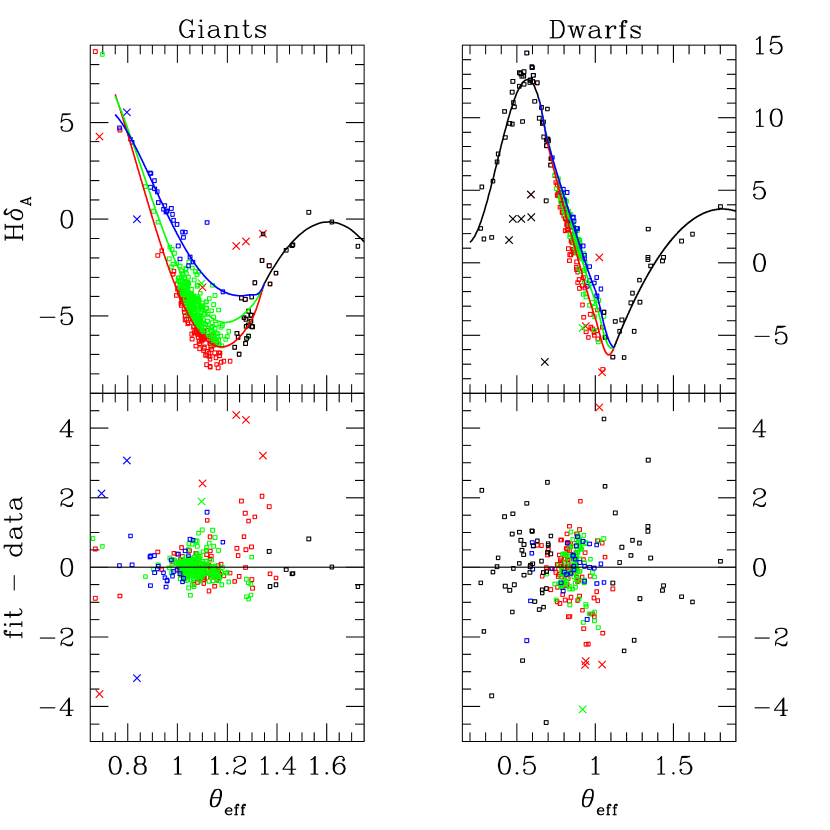
Figure 6.— a. Upper panels: fitting functions over-plotted on $H\delta_{A}$ measurements for dwarfs and giants, as indicated on top of each panel. The data are color-coded according to metallicity. Red dots correspond to [Fe/H] $\geq$ –0.1, green dots correspond to –0.6 $\leq$ [Fe/H] $<$ –0.1, and blue dots correspond to [Fe/H] $<$ –0.6. The red curves correspond to fitting functions computed for [Fe/H] = +0.1, the green to [Fe/H] = –0.35, and the blue to [Fe/H]=–1.0. A $T_{\rm eff}$ vs $\log g$ relation from Girardi et al. (2000)’s 5 Gyr old isochrone for solar metallicity is assumed. Black dots and lines are adopted for stars in regions of parameter space where the fits are [Fe/H]-independent. Bottom panels: Residuals of the fits. $\theta_{\rm eff}$ = 5040/$T_{\rm eff}$. In all plots crosses indicate stars that were rejected by the fitting routine. Similar figures for all the other indices are available electronically and will appear in the final version of the paper in the ApJS.

From the Figures and Tables it can be seen that the fits look fairly robust for G-K giants, and F-G dwarfs, which are the stellar types that are best represented in the spectral library. For these stars, reliable estimates of the behavior of the indices as a function of effective temperature, metallicity and surface gravity could be achieved. Outside these regions of parameter space, the low density of the spectral library (especially in the case of the very cool stars) and uncertainties in the stellar parameters made it very difficult to obtain estimates of the response of spectral indices to metallicity and surface gravity. Therefore, our fitting functions for all indices, except Fe5270 and Fe5335, are solely dependent on effective temperature for K-M dwarfs, M giants and B-A dwarfs. For those two indices we could not obtain fitting functions that would extend into the K-M dwarf regime without a moderately strong dependence on [Fe/H].

The boundaries listed in Tables7 are the ones adopted to produce the fits. Those attempting to reproduce our polynomial fits in Table 7 should adopt those boundaries as input in their programs. The latter boundaries should not be confused with those provided in Table 8 which specify the regions of parameter space within which the various fitting functions should be applied. Those are meant to be used by stellar population synthesis modelers wishing to adopt our fitting functions for the various Lick indices. The reader will notice that the boundaries in Table 8 are in general contained within those of Table 7, for a given index and stellar family. This is to ensure that application of our fitting functions be restricted to regions of parameter space where they are well constrained by the input stellar data. We strongly caution the reader against trusting extrapolations of the fitting functions away from the boundaries given in Table 8, as in many cases the functions behave in a strongly non-physical way outside the fitting region. In the case of the CN indices, we could not find polynomial functions capable of describing index behavior as a function of $T_{\rm eff}$and [Fe/H] in a satisfactory fashion in the metal-poor regime. Therefore we caution readers against trusting either the fitting functions or the single stellar population models for those indices below [Fe/H]=–1.0.

Blue indices tend to display a marked sensitivity to $\log g$ in stars hotter than $\sim$ 8000 K and for very low gravities ($\log g\mathrel{\hbox{\raise 2.15277pt\hbox{$<$}\hbox to0.0pt{\hss\lower 2.15277pt\hbox{$\sim$}}}}2$). All Balmer lines tend to be considerably weaker in the spectra of B-A super-giants than in that of dwarfs and giants of the same $T_{\rm eff}$. At such high $T_{\rm eff}$s Balmer lines are very strong, and their wings tend to be stronger for higher gravities. In the spectra of B-A dwarfs, the wings of the Balmer lines are so strong that they dominate the absorption at $\lambda\mathrel{\hbox{\raise 2.15277pt\hbox{$<$}\hbox to0.0pt{\hss\lower 2.15277pt\hbox{$\sim$}}}}4500$ K and have an impact on all other absorption line indices in that spectral region. As a result, indices like CN₁, CN₂, Ca4227, and G4300 present a dependence on $\log g$ that is similar in strength to that of the Balmer lines, but with opposite sign. Because the spectral library has just a handful of B-A super-giants, this effect could not be modelled in a reliable fashion, and we decided to exclude these very low surface gravity stars from our fits. Therefore, the fitting functions for hot stars should only be applied to stars with $\log g\mathrel{\hbox{\raise 2.15277pt\hbox{$>$}\hbox to0.0pt{\hss\lower 2.15277pt\hbox{$\sim$}}}}2$, for which no dependence of Balmer lines (and the other spectral indices) on $\log g$ could be perceived in our data.

Table 8Intervals of Applicability of the fitting functions

Index	$T_{\rm eff\,\,min}$ (K)	$T_{\rm eff\,\,max}$ (K)	$\log g_{\rm min}$	$\log g_{\rm max}$	[Fe/H]min	[Fe/H]max
$H\delta_{A}$ – G-K Giants	3790	6000	…	3.6	–1.3	+0.3
$H\delta_{A}$ – F-G Dwarfs	5100	7500	3.0	…	–2.0	+0.3
$H\delta_{A}$ – B-A Dwarfs	7500	18000	3.0	…	…	…
$H\delta_{A}$ – M Giants	2800	3790	…	3.6	…	…
$H\delta_{A}$ – K-M Dwarfs	3200	5100	4.0	…	…	…

4. Model Predictions for Single Stellar Populations

4.1. The Base Models

The fitting functions presented in Section 3 were combined with theoretical isochrones in order to produce predictions of integrated indices of single stellar populations. The isochrones employed were those from the Padova group for both the solar-scaled (Girardi et al. 2000) and $\alpha$-enhanced cases (Salasnich et al. 2000). There are several other groups producing state-of-the-art stellar evolutionary tracks and theoretical isochrones (e.g., Charbonnel et al. 1999, Yi et al. 2001, Kim et al. 2002, Pietrinferni et al. 2004, Jimenez et al. 2004) and it is very important to study the dependence of the results on the stellar evolution prescriptions. This will be discussed in a future paper. Absorption line indices and UBV absolute magnitudes were computed for the parameters listed in Table 9. In column (1) of Table 9 we list a model reference number, in columns (2) and (3) we list the mass fraction of elements heavier than He (Z) and that of He (Y). The iron abundance, overall metallicity, and mean $\alpha$-enhancement for the mixture adopted by the Padova group, given by [Fe/H], [Z/H] and [$\alpha$/Fe], are listed in columns (4) through (6). The mean $\alpha$-enhancement of the spectral library is listed in Column (7). Finally, column (8) contains the range of ages encompassed by each model set.

Throughout this paper we refer to the models summarized in Table 9 as our base models, which result from the mere combination of our fitting functions derived in Section 3 and the Padova isochrones. We note that, except for models 3 through 5, the $\alpha$-enhancement of the spectral library is inconsistent with that of the theoretical isochrones adopted (we assume here that a $\sim$ 0.1 dex mismatch is negligible). This condition is not unique to our base models. In fact, other well-known stellar population synthesis models in the literature (e.g., Worthey 1994, Vazdekis 1999, Bruzual & Charlot 2003, Le Borgne et al. 2004, Lee & Worthey 2005), which are based on similar combinations of theoretical isochrones and empirical stellar libraries, are afflicted by the same inconsistency. In principle, this issue can and has been addressed via adoption of the response functions of Tripicco & Bell (1995), Houdashelt et al. (2002), or Korn et al. (2005), as discussed above (e.g., Trager et al. 2000, Thomas et al. 2003a, Thomas et al. 2004, Lee & Worthey 2005). These models, however, are corrected for an assumed abundance pattern of the stars that make up the stellar library and therefore are also lacking in consistency. To our knowledge, the only attempts so far at full consistency between theoretical isochrones and stellar library are those of Coelho (2004) and this work. The former is based on synthetic spectra and the latter are discussed in Section 4.3.2.

Table 9Stellar Population Parameters of the Base Models

Model No.	Z	Y	[Fe/H]	[Z/H]	[$\alpha$/Fe]iso	[$\alpha$/Fe]lib	Age Range (Gyr)
1	0.001	0.23	–1.31	–1.31	0.0	+0.38	3.5–15.8
2	0.004	0.24	–0.71	–0.71	0.0	+0.20	3.5–15.8
3	0.008	0.25	–0.40	–0.40	0.0	+0.13	1.5–15.8
4	0.019	0.273	0.00	0.00	0.0	0.02	0.8–15.8
5	0.030	0.300	+0.22	+0.22	0.0	–0.02	0.8–15.8
6	0.008	0.25	–0.75	–0.40	+0.42	+0.20	3.5–15.8
7	0.019	0.273	–0.36	0.00	+0.42	+0.13	1.5–15.8
8	0.040	0.32	+0.01	+0.37	+0.42	0.02	0.8–15.8
9	0.070	0.39	+0.33	+0.68	+0.42	–0.02	0.8–15.8

Our computations were performed as follows. If $\Im$ is the line index in the integrated spectrum of a model single stellar population, it is given by

$$\Im=\sum_{i}^{N}\phi_{i}\,\,f_{i}\,\,I_{i}$$ (1)

when $\Im$ and $I_{i}$ are defined in terms of an equivalent width, and

$$\Im=-2.5\,\,\log\left(\sum_{i}^{N}\phi_{i}\,\,f_{i}\,\,10^{-0.4\,\,I_{i}}\right)$$ (2)

when $\Im$ and $I_{i}$ are defined in terms of a magnitude. In equations (1) and (2), $I_{i}$ is the index computed from our fitting functions for the stellar parameters corresponding to the $i$-th evolutionary stage. $N$ is the number of evolutionary stages in the theoretical isochrone adopted. $\phi_{i}$ is the relative number of stars at the $i$-th position in the isochrone, which is given by the initial mass function (IMF) of the stellar population. For simplicity, we adopt a power-law mass function, given by

$$\phi_{i}=\int A\,\,m_{i}^{1-x}dm$$ (3)

where $m_{i}$ is the mass at the $i$-th evolutionary stage in the isochrone and $A$ is a normalization constant which is chosen so that the entire stellar population has 1 $M_{\odot}$. The integration is performed within a narrow interval centered on $m_{i}$. For a Salpeter IMF, $x=1.35$.

The term $f_{i}$ in equations (1) and (2) gives the weight in flux for stars at the $i$th position of the isochrone. It is computed from interpolation between broad band absolute magnitudes to the index central wavelength. Absolute magnitudes in the U, B, and V bands were computed using the calibrations described in Paper I. Integrated magnitudes for single stellar populations in these bands were computed according to equation 2, with $f_{i}=1$ and making $I_{i}$ equal to the absolute magnitude of the $i$-th position in the isochrone. The results are provided in tables in the Appendix. Tables A2 and A3 provide Lick index predictions, and Tables A4 and A5 list predictions for UBV magnitudes/colors. In the following section we compare our predictions to those obtained when the fitting functions of Worthey et al. (1994) are employed.

4.2. New vs. Old Fitting Functions

Figure 7.— a. Comparison of model predictions based on our fitting functions (solid lines) and on those of Worthey et al. (1994, dashed lines), computed with the same set of isochrones. Metallicities are [Fe/H] = –1.3, –0.7, –0.4, 0.0, and +0.2. The arrows indicate the direction of increasing [Fe/H]. For the lowest metallicities, the Worthey et al. (1994) fitting functions are not defined for ages lower than 5 Gyr, but we decided to keep the comparisons for completeness.

Figure 7.— b.

Figure 7.— c.

Figure 7.— d.

We restrict our comparison to previous work on Lick/IDS fitting functions to those computed by G. Worthey and collaborators, because they are available for all the indices studied here and are based on a very comprehensive spectral library. Moreover, they are the most widely used fitting functions in stellar population synthesis work.

In order to assess the impact of our new fitting functions on model predictions we proceeded as follows. We computed integrated line indices for models 1 through 5 in Table 9 adopting our own fitting functions and those of Worthey et al. (1994) and Worthey & Ottaviani (1997) (henceforth simply Worthey et al.). In this way we isolate the effect on model predictions due only to the adoption of our new fitting functions.

The two sets of model predictions are compared in Figures 7a through 7d for all indices. The indices computed adopting the Worthey et al. fitting functions were brought into our system of EWs using the zero-points listed in Table 1. In each panel arrows indicate in which sense model metallicity varies, to help the reader identify the models with different [Fe/H].

The overall agreement between the two sets of computations is good. Not unexpectedly, most of the differences are found at low metallicity, where both sets of fitting functions are more uncertain. Amongst the Balmer lines, the most important differences are found for $H\beta$. This index is more metallicity-dependent when the Worthey et al. fitting functions are adopted. This is a very interesting result that serves to illustrate how improvements in the accuracy of stellar data (both stellar parameters and spectra) can cause a noticeable improvement in model predictions. In Figure 8 we compare the input data used in the computation of both sets of fitting functions. In the upper panel, $H\beta$ and $T_{\rm eff}$ from the Worthey et al. (1994) are plotted against each other for G and K giants and the same plot is repeated in the lower panel using our data. Stars in two ranges of metallicity are plotted in order to highlight the dependence of $H\beta$ on this parameter. Stars with [Fe/H] $>$ 0 are plotted with solid squares and stars with [Fe/H] $<$ –0.3 with open squares. A dependence of $H\beta$ on metallicity, whereby at fixed $T_{\rm eff}$ the index becomes stronger for higher [Fe/H], can be seen in both data-sets, but is far more clear-cut in our data than in those of Worthey et al. (1994). As a result, we can estimate the dependence of $H\beta$ on metallicity in stellar spectra more accurately. We find that $H\beta$ in the spectra of GK giants responds to variations in [Fe/H] roughly twice as strongly than predicted by Worthey et al. (1994) in the sense that, we repeat, $H\beta$ becomes stronger for higher metallicity. On the other hand, we know that higher metallicity systems tend to have cooler turn-offs, which tends to produce weaker $H\beta$. Therefore, the two above effects tend to cancel out, with the net result that the index in integrated spectra of stellar populations becomes less sensitive to [Fe/H] than predicted by former models. As a result, the new fitting functions show that $H\beta$ is a better age indicator (i.e., less sensitive to [Fe/H]) than previously thought.

Figure 8.— Top panel: $H\beta$ against $T_{\rm eff}$ for giant stars in the Worthey et al. (1994) database. Bottom panel: Same for our data. Open squares: stars with [Fe/H] $<$ –0.3. Filled squares: stars with [Fe/H] $>$ 0. The improvement on both index measurements and stellar parameters allows us to estimate the dependence of the index on [Fe/H] more accurately.

The Fe indices are extremely important because they are mostly sensitive to the abundance of iron (Tripicco & Bell 1995), thus providing a close estimate of the mean [Fe/H] of an integrated stellar population. In Figure 7 we compare our model predictions to those based on the Worthey et al. fitting functions for all the Fe indices modelled here. Agreement between the two sets of fitting functions is good for Fe4383 and Fe5335. The most important differences are found for Fe5270 at metallicities below solar. In Figure 9 we compare the two sets of fitting functions for dwarfs with [Fe/H]=–0.4. Our data and fitting functions are represented respectively by the solid squares and thick solid line. The open squares and thin line indicate Worthey et al. data and fitting functions. Only dwarfs with [Fe/H] = –0.4 $\pm$ 0.15 are plotted. As in the case of Figure 8 the quality of the new stellar data is quite superior, as can be seen by the lower scatter in the solid squares. That of course makes it far easier to compute an accurate fitting function for the index. It can be seen that our new set of fitting functions provides a better description of the data for mildly metal-poor dwarfs. The latter accounts for roughly 2/3 of the mismatch seen in Figure 7. The rest of the mismatch is due to smaller differences in the fitting functions for giant stars.

Another interesting case is that of indices that are strongly sensitive to surface gravity, such as Mg₂, Mg $b$, and Ca4227, for which the Worthey et al. al fitting functions yield higher values for solar metallicity at all ages. This is because the line strengths in the spectra of giants are stronger according to the Worthey et al. fitting functions. This point is illustrated in Figure 10 where the two sets of fitting functions are compared with Mg₂ data for M 67 stars in an Mg₂-magnitude diagram. The data come from Paper III, whereas the isochrones were computed by combining the two sets of fitting functions with the Girardi et al. (2000) isochrone for an age of 3.5 Gyr and solar metallicity. The latter was shown to provide an excellent match to the color-magnitude diagram of the cluster (see Paper III for details). It can be seen from this Figure that, when the Worthey et al. fitting functions are adopted the index is over-predicted by $\sim$ 0.05 mag throughout most of the red-giant sequence and also at the horizontal branch (thick lines). A similar behavior is seen for Mg $b$ and Ca4227.

It is also important to point out that the two Mg indices have a markedly different sensitivity to IMF variations. While Mg₂ is strongly sensitive to the contribution of K dwarfs, Mg $b$ is nearly insensitive. This can be understood by looking at Figure 11, where we plot measurements of the two indices in our library star spectra as a function of $T_{\rm eff}$  for dwarf and giant stars. For K stars (5500 $\mathrel{\hbox{\raise 2.15277pt\hbox{$>$}\hbox to0.0pt{\hss\lower 2.15277pt\hbox{$\sim$}}}}$ $T_{\rm eff}$ $\mathrel{\hbox{\raise 2.15277pt\hbox{$>$}\hbox to0.0pt{\hss\lower 2.15277pt\hbox{$\sim$}}}}$ 4000 K), both indices respond to $T_{\rm eff}$ and $\log g$ in essentially the same way. In particular, they tend to be stronger in K dwarfs, because both the Mg II lines and the MgH band-head included in the Mg₂ passband are stronger for higher surface gravities (Barbuy, Erdelyi-Mendes & Milone 1992). At lower $T_{\rm eff}$, presumably because the Mg II lines saturate, the indices cease to increase for lower temperatures and its dependence on $\log g$ also becomes weaker. In the M-star regime ($T_{\rm eff}$ $\mathrel{\hbox{\raise 2.15277pt\hbox{$<$}\hbox to0.0pt{\hss\lower 2.15277pt\hbox{$\sim$}}}}$ 4000 K) the two indices behave in drastically different ways. While Mg $b$ becomes much stronger in giants than in dwarfs, Mg₂ is very little dependent on surface gravity. The reason for this behavior is that, as pointed out in Paper III, Mg $b$ is severely affected by a TiO band, which is so strong in the spectra of M giants that Mg $b$ becomes essentially a TiO indicator (see Figure 3 in Paper III, for details). Because TiO bands are very strongly sensitive to $\log g$  being stronger in giants than in dwarfs of the same $T_{\rm eff}$ (Schiavon & Barbuy 1999, Schiavon 1998), the Mg $b$ index becomes much stronger in the former than in the latter. The Mg₂ index, on the other hand, is far less influenced by TiO lines, because they affect both the pseudo-continuum and index passband in similar ways. This result has an interesting ramification, namely, that Mg₂ is an IMF-sensitive index, and Mg $b$ is nearly unaffected by IMF variations. This can be understood by looking at Figure 11. The Mg₂ index is IMF-sensitive because it is much stronger in dwarf stars, so that it tends to be stronger for dwarf-enriched IMFs. The same is not true for Mg $b$, because the index is so strong in cool giants that its sensitivity to the contribution by K-dwarfs is washed away. As a result, when used in combination, the Mg₂ and Mg $b$ indices can be used to constrain both the magnesium abundance and the shape of the IMF in the low-mass regime. We return to this topic in Section 5.2.2.

There is a caveat here that needs to be highlighted. When we first computed the model predictions with our fitting functions we obtained too weak Mg₂ values for stars in the lower giant branch ($12.5\mathrel{\hbox{\raise 2.15277pt\hbox{$<$}\hbox to0.0pt{\hss\lower 2.15277pt\hbox{$\sim$}}}}$ V $\mathrel{\hbox{\raise 2.15277pt\hbox{$<$}\hbox to0.0pt{\hss\lower 2.15277pt\hbox{$\sim$}}}}11.5$ in M67, cf. Figure 10). That region of the diagram is inhabited by K stars with intermediate surface gravities ($3.0\mathrel{\hbox{\raise 2.15277pt\hbox{$<$}\hbox to0.0pt{\hss\lower 2.15277pt\hbox{$\sim$}}}}\log g\mathrel{\hbox{\raise 2.15277pt\hbox{$<$}\hbox to0.0pt{\hss\lower 2.15277pt\hbox{$\sim$}}}}3.6$), which are scarce in our spectral library. Therefore, our fitting functions are poorly constrained in this region of stellar parameter space. For that reason, we decided to interpolate our predictions for gravity-sensitive indices, using index-magnitude diagrams such as the one shown in Figure 10 to check the quality of the interpolations.

In Summary, we conclude that our fitting functions are generally in good agreement with those of Worthey et al. (1994). The differences found are mostly due to the better quality of our data and the higher accuracy of our stellar parameters. The latter validates our efforts to refine the stellar parameter determinations, as described in Section 2.3.

4.3. Abundance-Ratio Effects

Absorption-line strengths in the integrated spectrum of a single stellar population are affected by its abundance pattern for two main reasons: i) the effective temperatures and, potentially, the luminosities of two stars with same mass, age, helium abundance, and metallicity, but different abundance patterns, are different, and as a result the spectra of these two stars are different; ii) the spectra of two stars that occupy the same position on the HR diagram and have the same metallicity are different if they have different abundance patterns. The effect of the abundance mix on the effective temperature of a given star is due to the relative contribution of different elements to the overall opacity of the stellar interior. Oxygen is the most important metallic source of opacity at the high temperatures prevalent in the stellar interiors (Vandenberg & Bell 2001). In the outer layers, iron is the predominant metal source of opacity for FGK stars, which dominate the light of single stellar populations in the spectral region of relevance for this study. It is therefore fair to say that the effect of abundance ratios on the positions of stars in the HR diagram is dictated by the relative abundances of oxygen and iron. Line strengths, on the other hand, can be strongly affected by the individual abundances of elements which are not optically active enough to produce a substantial change in the star’s structure. Two stars with the same mass, age, metallicity, and helium abundance, and whose abundance patterns are the same except, for instance, for their calcium abundances, have virtually the same temperature and luminosity, and their spectra will be essentially the same, except for differences in the strengths of lines due to atomic calcium or due to molecules involving calcium, such as calcium hydride.

Since the realization that the chemical composition of stars in giant early-type galaxies is enhanced in light elements (e.g., Peterson 1976, O’Connell 1980, Peletier 1989, Worthey et al. 1992), a great deal of effort has been invested into producing realistic models with an $\alpha$-enhanced abundance pattern. These efforts branch out in two major directions, aimed at accounting for the two major effects listed above: i) computation of stellar evolutionary tracks for metal-rich stars incorporating an $\alpha$-enhanced mixture (e.g., Weiss et al. 1995, Salasnich et al. 2000, Kim et al. 2002) in order to assess the impact of $\alpha$-enhancement on model predictions, and ii) estimating the effect of the abundance pattern onto stellar spectra and line indices (e.g., Barbuy 1994, Tripicco & Bell 1995, Paper I, Barbuy et al. 2003, Coelho 2004, Mendes de Oliveira et al. 2005, Korn, Maraston & Thomas 2005), using spectrum synthesis from model stellar atmospheres.

Figure 9.— $T_{\rm eff}$ against Fe5270 for K-F dwarfs. Our data are shown as filled squares, and Worthey et al. data as open squares. Our fitting function is shown as a thick line and that of Worthey et al. as a thin line. Only stars with [Fe/H] = –0.4 $\pm$ 0.15 are displayed and the fitting functions were computed for [Fe/H] = –0.4.

Before comparing model predictions with data in Section 5, it is interesting to discuss the impact of abundance ratios on model predictions. For simplicity, throughout this paper we refer to i) above as evolutionary abundance-ratio effects and to ii) as spectroscopic abundance-ratio effects. In Section 4.3.1, we examine evolutionary abundance ratio effects, which are those stemming from the influence of the abundance mixture on the luminosity and effective temperature of a star of given mass, metallicity and evolutionary stage. Spectroscopic abundance-ratio effects are considered in Section 4.3.2.

4.3.1 Evolutionary Abundance-Ratio Effects

In Figure 12 our models for single stellar populations are displayed in the $H\beta$ vs. $<Fe>$ (upper panel) and $H\delta_{F}$ vs. $<Fe>$ planes. These indices illustrate very well the general effect of $\alpha$-enhanced isochrones on Balmer and metal lines. In both panels, black lines indicate models computed with the $\alpha$-enhanced Padova isochrones (Salasnich et al. 2000) and gray lines those with the solar-scaled isochrones (Girardi et al. 2000). The ages of the models displayed are, from top to bottom, 1.2, 1.5, 2.5, 3.5, 7.9, and 14.1 Gyr. For clarity, we restrict the comparison to those amongst the two sets of models computed with similar [Fe/H] values (2 through 4 and 6 through 8 in Table 9). Solid lines connect same-[Fe/H] models, and dotted lines connect same-age models. The models for 3.5 Gyr are plotted with a long-dashed line, for clarity.

Figure 10.— An Mg₂-magnitude diagram for stars from M 67. The thin line shows computations adopting the Girardi et al. (2000) isochrone for 3.5 Gyr and solar metallicity and the Worthey et al. fitting functions. The thick lines were obtained using our fitting functions.

The main difference between models computed with solar-scaled and $\alpha$-enhanced isochrones is that the latter tend to predict weaker Balmer lines and slightly stronger metal lines, for the same age and [Fe/H]. This is because $\alpha$-enhanced turn-off stars are cooler and fainter than their solar-scaled counterparts at fixed [Fe/H], due to increased opacity, especially due to oxygen, in the stellar interior (e.g., Vandenberg & Bell 2001). In particular, the mixture adopted by Salasnich et al. in their $\alpha$-enhanced tracks is enhanced in [O/Fe] by +0.5 dex relative to solar. As a combination of the temperature effects on Balmer and metal lines, the models based on $\alpha$-enhanced isochrones appear to “slide” relative to the solar-scaled models along same-[Fe/H] lines, towards weaker $H\beta$. The final effect is that, for a given data point, $\alpha$-enhanced models predict younger ages but, interestingly, essentially the same [Fe/H]. For the mixture adopted by Salasnich et al. (Table 9) the age effect is of the order of $\sim$ 1 Gyr at intermediate ages ($\sim$ 4 Gyr), and as large as $\sim$ 3 Gyr for the ages of the oldest globular clusters ($\sim$ 14 Gyr). This effect, together with our improvement to the fitting function of the $H\beta$ index, leads to significantly younger ages for old stellar populations, thus ameliorating a long-standing problem, namely, that stellar population synthesis models tend to predict too old ages for the oldest stellar systems (e.g., Cohen, Blakeslee & Rhyzov 1998, Gibson et al. 1999, Vazdekis et al. 2001, Papers I and II, Proctor, Forbes & Beasley 2004, Lee & Worthey 2005). This issue is addressed further in Section 5.

We also note that $H\delta_{F}$ is substantially less affected than $H\beta$ especially for the oldest models. Comparing the two models for 14 Gyr in the bottom panel of Figure 12 we see that the variation in $H\delta_{F}$ corresponds to less than $\mathrel{\hbox{\raise 2.15277pt\hbox{$<$}\hbox to0.0pt{\hss\lower 2.15277pt\hbox{$\sim$}}}}$ 1 Gyr, compared to $H\beta$, whose variation amounts to $\mathrel{\hbox{\raise 2.15277pt\hbox{$<$}\hbox to0.0pt{\hss\lower 2.15277pt\hbox{$\sim$}}}}$ 3 Gyr.

Figure 11.— Comparison between the behavior of Mg $b$ (lower panel) and Mg₂ as a function of $T_{\rm eff}$ and $\log g$. In both panels, measurements taken in the spectra of the library stars are plotted as a function of $T_{\rm eff}$ for dwarf and giant stars, as indicated in the upper panel. For K stars (4000 $\mathrel{\hbox{\raise 2.15277pt\hbox{$<$}\hbox to0.0pt{\hss\lower 2.15277pt\hbox{$\sim$}}}}$ $T_{\rm eff}$ $\mathrel{\hbox{\raise 2.15277pt\hbox{$<$}\hbox to0.0pt{\hss\lower 2.15277pt\hbox{$\sim$}}}}$ 5500 K), the behavior of the two indices as a function of both stellar parameters is essentially the same. Both indices are strongly sensitive to temperature and tend to be stronger in dwarf stars. For cooler, M stars, Mg $b$ tends to be much stronger in giants, unlike Mg₂, which is less dependent on surface gravity. This is due to the effect of TiO bands on Mg $b$. See text for details.

We would like to call the reader’s attention to an important new development. After submission of the first version of this paper, Weiss et al. (2006) showed that there was an error in the opacity tables adopted in the calculation of the Padova $\alpha$-enhanced evolutionary tracks, by (Salasnich et al. 2000). This error is such that the temperatures at the red giant branch and turnoff were overestimated by 200 and 100 K, respectively, for solar metallicity. Even though new isochrones with the mixture adopted by Salasnich et al. are not available, we simulated the effect of the corrected opacity tables by artificially changing the temperatures of giant and turn-off stars uniformly by 200 and 100 K in Salasnich et al. isochrones with Z=0.04 (nearly solar [Fe/H]). As a result, Balmer lines get weaker and metal lines get stronger. The change in $H\beta$ ($H\delta_{F}$) is of the order of $\sim$ –0.15 (–0.1) ${\rm\AA}$. Because Balmer lines would tend to get weaker in the models, ages according to these “corrected” $\alpha$-enhanced isochrones would get younger, thus accentuating the differences seen in Figure 12. The effect would be of the order of $\sim$ 2.5 (1) Gyr for an 11 (3) Gyr-old stellar population, in the case of $H\beta$. Ages according to $H\delta_{F}$ would get younger by $\sim$ 1.2 (0.5) Gyr for 11 (3) Gyr-old stellar populations. The change in $<Fe>$ is of the order of $\sim$ +0.14 ${\rm\AA}$ and it is such that models change along a line of constant [Fe/H] in the $<Fe>$-$H\beta$ plane. More definitive numbers have to await publication of $\alpha$-enhanced theoretical isochrones computed on the basis of updated opacities.

According to Weiss (2006, private communication), adoption of new opacities has a less important impact for lower metallicities. For instance, in the case of the metallicity of 47 Tuc, changes in age would be of the order of $\sim$ 1.5 Gyr and essentially zero in [Fe/H], so that our discussion in Paper II remains entirely valid.

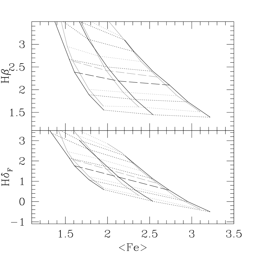
Figure 12.— Effect of adopting $\alpha$-enhanced isochrone (dark lines), as opposed to solar-scaled ones (gray lines) on predictions for $<Fe>$ and Balmer lines for single stellar populations. The ages shown are, from top to bottom, 1.2, 1.5, 2.5, 3.5, 7.9, and 14.1 Gyr. The values for [Fe/H] are –0.8 (–0.7 for solid lines), –0.4, and 0.0. The $\alpha$ enhanced isochrones yield weaker Balmer lines and slightly weaker $<Fe>$ for the same age and metallicity. Note that the effect is stronger on $H\beta$ than on $H\delta_{F}$.

4.3.2 Spectroscopic Abundance-Ratio Effects

In the previous section we studied how the adoption of $\alpha$-enhanced isochrones affects our model predictions. Here we show how the sensitivity of line indices to the various elemental abundances alters the model predictions. The method, first proposed by Trager et al. (2000) and further developed by Thomas et al. (2003a) and Korn et al. (2005), is based on estimates of how line indices in the spectra of three types of stars with relevant atmospheric parameters (a turnoff, a giant, and a lower main sequence star) change as a function of variations of the abundances of individual elements. Briefly, the method goes as follows. Initially, synthetic spectra are computed on the basis of model photospheres, for the three stellar types above, assuming a solar-scaled abundance pattern. For each stellar type, a new spectrum is then computed by varying the abundance of a single element. The impact of this sole elemental abundance on all spectral indices is assessed by comparing line indices measured in both the solar-scaled synthetic spectrum and that computed with the altered abundance pattern. The procedure is repeated for all the chemical abundances of relevance in the spectral region of interest and the final results are summarized in the form of sensitivity tables, such as those provided by Tripicco & Bell (1995) and more recently updated by Korn et al. (2005) and Serven, Worthey & Briley (2005). The sensitivity tables are used to estimate incremental changes in absorption line indices as a function of stellar parameters, which are integrated along the theoretical isochrone in order to produce integrated line strength predictions for any desired abundance pattern.

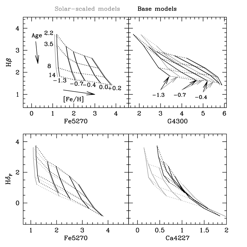
Figure 13.— Comparison between solar-scaled (gray) and base models (dark) on a few representative index-index plots. Upper Left: Both $H\beta$ and Fe5270 are essentially insensitive to abundance ratio variations. Upper Right: G4300 is stronger in solar-scaled than in the base models for [Fe/H] $\leq$ –0.4, because the latter have higher oxygen abundances (see text). Lower Left: $H\delta_{F}$ is weaker in solar-scaled than in the base models for [Fe/H] $\mathrel{\hbox{\raise 2.15277pt\hbox{$<$}\hbox to0.0pt{\hss\lower 2.15277pt\hbox{$\sim$}}}}$–0.4, because at these metallicities the base models have higher magnesium and calcium abundances, indicating that there are lines due to these two elements in the $H\delta_{F}$ index passband. Lower Right: The Ca4227 index is much weaker in solar-scaled than in the base models for [Fe/H]$\mathrel{\hbox{\raise 2.15277pt\hbox{$<$}\hbox to0.0pt{\hss\lower 2.15277pt\hbox{$\sim$}}}}$–0.4, having similar strength for [Fe/H]=0 and +0.2. This reflects the fact that the base models have higher calcium abundance than solar-scaled models for metallicities below solar (see Table 6).

In this section we discuss the behavior of all the line indices studied in this paper as a function of the most important elements affecting their strengths in the range of stellar population parameters considered. In order to study this effect in isolation from that discussed in the previous Section, we perform calculations based on the same set of isochrones (Padova, solar-scaled), but varying the line indices according to their sensitivity to abundance ratio variations. The sensitivity tables used are those by Korn et al. (2005).

Solar-scaled vs. Base Models

The starting point for this discussion are the base models, which are summarized in Table 9. Models for any abundance pattern can be calculated relative to the base models in a differential fashion. As a first step, we generate solar-scaled models, for which [X_i/Fe] = 0 for all elements X_i, and at all values of [Fe/H]. These models are generated by correcting the base models from the abundance pattern listed in Table 6 to a solar-scaled abundance pattern. Because metallicity in our models is cast in terms of [Fe/H], this parameter is kept fixed whenever we calculate a model with a new abundance pattern. For instance, according to Table 6, if one wants to compute solar-scaled models with [Fe/H]=–0.4, one needs to correct the indices in the [Fe/H]=–0.4 base models for abundance ratio variations of $\Delta$ [O/Fe]=–0.2, $\Delta$ [Mg/Fe]=–0.13, $\Delta$ [Ca/Fe]=–0.06, and $\Delta$ [Ti/Fe]=–0.11. Those are the elemental abundance variations needed to bring the abundance ratios in Table 6 to [X_i/Fe]=0 (no need to perform any correction for variations of [C/Fe] and [N/Fe], as these ratios are solar in the spectral library for all values of [Fe/H]). As a result, two models with same [Fe/H] and different abundance patterns have different total abundances [Z/H]. This is different from the procedure followed by Trager et al. (2000) and Thomas et al. (2003a), who cast their models in terms of [Z/H], so that their $\alpha$-enhanced models have lower [Fe/H] for fixed [Z/H].

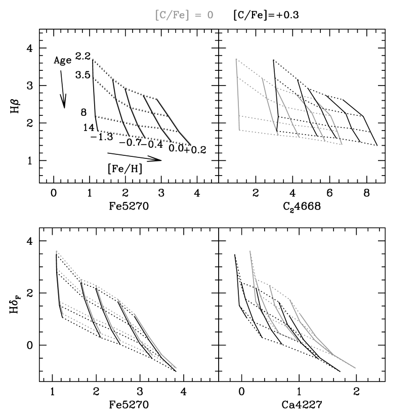
Figure 14.— Comparison between solar-scaled (gray) and carbon-enhanced (dark) models. Upper Left: This panel shows that $H\beta$ and Fe5270 are virtually insensitive to carbon abundance variations. Upper Right: As expected, C₂4668 is strongly sensitive to carbon abundance variations. It is the best carbon-abundance indicator modeled in this paper. Lower Left: $H\delta_{F}$ is very mildly sensitive to carbon abundance variations, in spite of its being surrounded by CN lines (see text). Lower Right: The Ca4227 index is very sensitive to carbon, being stronger in lower carbon-abundance models. This is due to the presence of a CN band-head on the index blue pseudo-continuum, as pointed out by Prochaska et al. (2005, see discussion in the text).

The result is illustrated in Figure 13, where base and solar-scaled models (dark and gray lines, respectively) are compared in four representative index-index planes. Because the abundance pattern characteristic of the base models only differs importantly from solar-scaled for [Fe/H]$\leq$–0.4, we only expect to find differences in this iron abundance interval. In the upper left panel, the two sets of models are compared in the Fe5270-$H\beta$ plane, where there is hardly any difference between solar-scaled and base models. The reason is that both indices are very little affected by variations of the abundances of any elements other than Fe. The only exception happens at [Fe/H]=–1.3, where the base models have slightly stronger Fe5270, due to the presence of titanium and calcium lines in the index passband. Because [Fe/H] is kept fixed when switching from base to solar-scaled models, the two model sets are virtually identical in the Fe5270-$H\beta$ plane. The same is not the case in the upper-right panel, where models are compared in the G4300-$H\beta$ plane, where the G4300 index appears to display a complex behavior as a function of [Fe/H]. As expected, the index is unchanged for models with [Fe/H]=0 and +0.2, but it becomes stronger in solar-scaled models for lower [Fe/H] values (same-[Fe/H] models are indicated with arrows, for clarity). The G4300 index is mostly a carbon abundance indicator, because of the presence of a strong vibrational band of the CH molecule in the index passband. However, Table 6 tells us that [C/Fe] is solar in the base models, so that it is the same for all [Fe/H] in both sets of models. However, the G4300 index is also affected, in an indirect way, by oxygen abundance variations, in the sense that the index tends to be weaker for higher oxygen abundances. Because the abundance of oxygen is lower in the solar-scaled than in the base models, the former have stronger G4300 for fixed [Fe/H]. One can also conclude from this plot that the G4300 index is very strongly sensitive to age, which can be seen by the fact that the model grids are very far from orthogonal. On the other hand its sensitivity to metallicity and/or carbon abundance is relatively weak, as can be seen by the fact that model lines for different values of [Fe/H] are packed very close together, especially for [Fe/H] $\geq$ –0.7. As a result, the G4300 index is a less than ideal carbon abundance indicator, which is the reason why we decided to include the C₂4668 index in our models. A more detailed discussion of this issue will be presented in Graves & Schiavon (2006, in preparation).

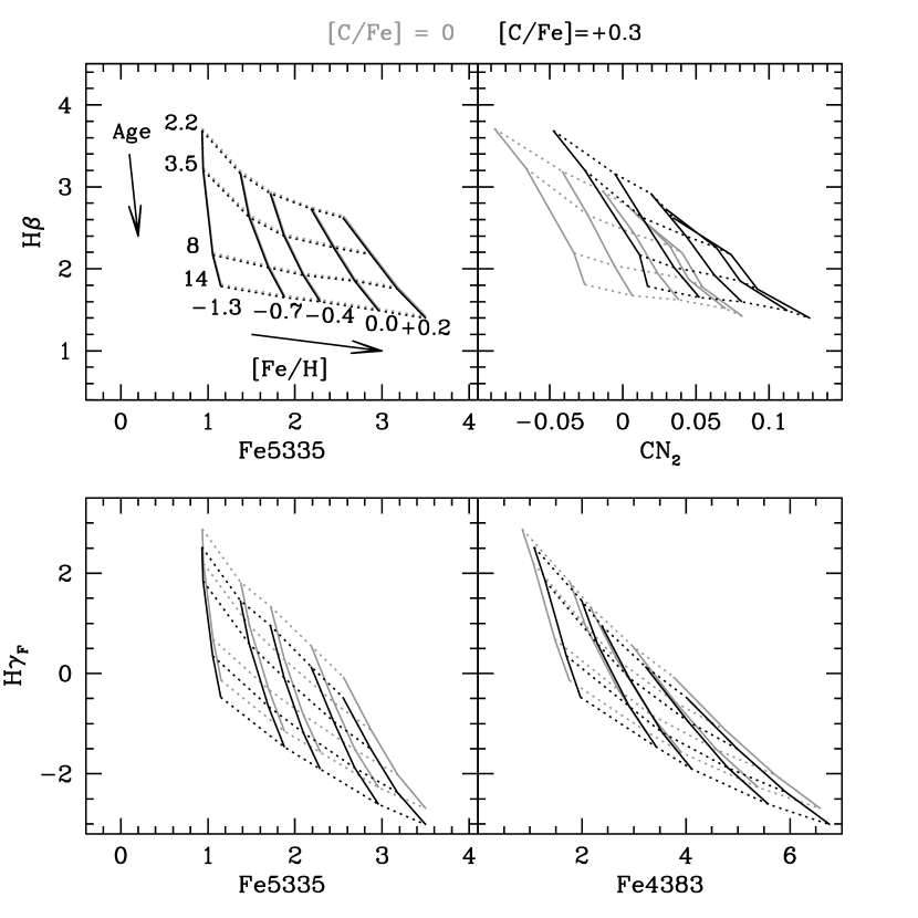
Figure 15.— Figure 14 continued. Upper Left: This panel shows that the Fe5335 index is also essentially insensitive to carbon abundance variations. Upper Right: As expected, CN₂ is very sensitive to carbon, being substantially stronger for higher carbon abundances. This index is also sensitive to nitrogen, but not as strongly as to carbon. Lower Left: This plot shows how $H\gamma_{F}$ is affected by carbon abundance variations. It gets weaker for higher carbon, due to contamination of the index pseudo-continuum by CH lines. Lower Right: The Fe4383 index is almost insensitive to carbon. The index becomes only slightly stronger for higher carbon abundances. This effect is also due to the presence of CH lines in the index passband.

In the lower left panel, models are compared in the Fe5270-$H\delta_{F}$ plane. It can be seen that $H\delta_{F}$ is slightly weaker in solar-scaled models for [Fe/H]$\leq$–0.4. This is because the passband of the index includes lines due to calcium and magnesium, whose abundances are higher in the base models at these lower values of [Fe/H]. Finally, in the lower-right panel, models are compared in the Ca4227-$H\delta_{F}$ plane, which allows us to investigate the behavior of the Ca4227 index as a function of abundance ratios. As expected, base models have stronger Ca4227 at [Fe/H]$\leq$–0.4 than solar-scaled models, given that the latter have lower calcium abundances. The effect is in fact enhanced by the strengthening of CN bands in the solar-scaled models, due to their lower oxygen abundances, for reasons that will be discussed in the next section.

Effects of Carbon Enhancement

The blue spectra of G and K-type stars is pervaded by weak to moderately strong absorption lines due to the CN and CH molecules. That is in fact one of the most important challenges for the reliable modeling of the spectra of old/intermediate-age stellar populations in the blue (e.g., Vazdekis 1999, Paper I, Prochaska, Rose & Schiavon 2005, Prochaska et al. 2006). For that reason, it is important to investigate the effects of variations of the abundances of carbon and nitrogen on blue spectral indices.

In Figures 14 and 15 we compare solar-scaled models with models where only the abundance of carbon is enhanced by +0.3 dex. In the upper left panel of Figure 14, the models are compared in the Fe5270-$H\beta$ plane, where it can be seen that the two indices are essentially insensitive to carbon abundance variations. In the upper right panel, on the other hand, one can see that the C₂4668 index is extremely sensitive to carbon abundance variations, indeed, far more sensitive than the G4300 index. This is not unexpected, given that the concentration of the C₂ molecule in stellar atmospheres depends quadratically on the abundance of carbon, while that of CH depends only linearly on that parameter. In the lower left panel, one can see that $H\delta_{F}$ is very little affected by carbon abundance variations, in spite of the fact that the index is immersed in a thick forest of CN lines. This has been discussed in Paper I, where it was shown that the small sensitivity of $H\delta_{F}$ to carbon abundance variations was due to the the fact that the effect of CN lines in both the index passband and pseudo-continuum regions is partially cancelled. For a detailed discussion of the impact of CN lines on $H\delta$ measurements, see Prochaska et al. (2006). In the lower right panel of Figure 14 the models are compared in the Ca4227-$H\delta_{F}$ plane, where it can be seen that the Ca4227 index is strongly sensitive to carbon abundance variations, in the sense that the index becomes substantially weaker for increasing carbon abundances. This effect has been studied in detail by Prochaska et al. (2005) and it is due to the contamination of the blue pseudo-continuum of the index by a CN band-head. An increase in carbon abundance leads to a depression of the blue continuum and, consequently, to an artificially lower Ca4227 index. Prochaska et al. (2005) defined a new index, Ca4227_r, which is far less affected by CN contamination. Analyzing a large sample of nearby early-type galaxies, they showed that this new index presents a correlation with velocity dispersion ($\sigma$) which is much stronger than that of the Lick Ca4227 index, resembling the behavior of other $\alpha$-elements, such as magnesium. In subsequent sections, we will show that when the effect of CN lines is accounted for, one can extract reliable calcium abundances from measurements of the Lick Ca4227 index.

Figure 15 illustrates the effect of carbon abundances on another set of relevant Lick indices. In the upper left panel, one can see that, like Fe5270, the Fe5335 index is unchanged when carbon is varied. The same is true of the Fe5015 index (not shown). In the upper right panel, on the other hand, one can see that the CN₂ index is very sensitive to carbon abundance, as expected. It is also sensitive to nitrogen abundance, to a lesser extent. In the lower left panel, the models are compared in the Fe5335-$H\gamma_{F}$ plane, where it can be seen that this Balmer line is somewhat affected by carbon, in the sense that $H\gamma_{F}$ is weaker for higher carbon abundances. This is due to contamination of the index pseudo-continuum by CH lines. Finally, in the lower right panel, one can see that the Fe4383 index is only very mildly affected by carbon abundances, in the sense that the index becomes stronger for higher carbon, due to contamination of the index passband by CH lines.

Nitrogen abundance variations affect CN lines and therefore indirectly affect a number of indices, most notably $H\delta_{F}$, $H\delta_{A}$, and Ca4227. Since the variation of CN lines as a function of carbon abundances and their impact on line indices has been discussed here and since CN lines respond similarly to carbon and nitrogen (see Korn et al. 2005), there is no need to show model variations as a function of nitrogen here.

In summary, we find that, among the Balmer line indices, the only ones that are affected by the abundance of carbon are the $H\gamma_{F}$ and $H\gamma_{A}$ indices. Application of a solar-scaled model to $H\gamma$ measurements taken in the spectrum of a carbon-enhanced stellar population would lead to an age overestimate. For a stellar population with [C/Fe]=+0.3 the effect would be of the order of $\sim$ 5 (1) Gyr for ages of $\sim$ 10 (2) Gyr. Amongst the metal line indices, the ones that are the most sensitive to carbon are C₂4668, G4300, CN₁, CN₂, and Ca4227 (the latter due to a spurious contamination of the index blue pseudo-continuum). The cleanest carbon abundance indicator studied in this work is C₂4668, as it is solely dependent on the abundances of carbon and iron, and (very weakly) on age. The CN indices are also very strongly dependent on carbon, but are also sensitive to nitrogen, as expected. The iron indices Fe5270, Fe5335, and Fe5015 are free of the influence of carbon abundance variations, while the Fe4383 index is slightly affected by them.

Effects of $\alpha$-Element Enhancement

The abundance of $\alpha$ elements relative to that of iron provides some of the most fundamental clues available on the history of star formation and chemical enrichment of galaxies (e.g., Matteucci & Tornambé 1987, Wheeler et al. 1989, Peletier 1989, Worthey et al. 1992, Edvardsson et al. 1993, McWilliam 1997, Worthey 1998, Trager et al. 2000). Therefore, it is crucially important to understand how indices respond to variations of $\alpha$-element abundances, so that the latter can be estimated from index measurements taken in the integrated spectra of galaxies. In Figures 16 and 17 we contrast solar-scaled and $\alpha$-enhanced models in a number of index-index diagrams. The $\alpha$-enhanced models are computed by increasing by +0.3 dex the abundances of oxygen, magnesium, calcium, sodium, silicon, and titanium. We emphasize again that these computations do not take into account the effect of oxygen abundances in the stellar interiors (see Section 4.3.1), but only their spectroscopic effect, which is mostly due to changes in the strengths of carbon-based molecules, due to the impact of oxygen abundances on the concentration of free carbon atoms via the dissociation equilibrium of the CO molecule. As another caveat, we note that indices capable of constraining the abundances of sodium, silicon, or titanium are not modelled in this work. However, these abundances only have a small impact on the strengths of some of the indices modelled here (see Korn et al. 2005 for details), so we choose to force these abundances to track those of the other $\alpha$-elements.

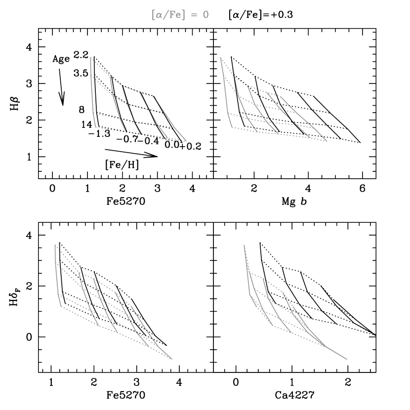
Figure 16.— Comparison between solar-scaled and $\alpha$-enhanced models. Upper Left: This panel shows that $H\beta$ is insensitive to spectroscopic $\alpha$-enhancement, while Fe5270 is only very mildly sensitive, and only at very low [Fe/H]. Upper Right: As expected, the Mg $b$ index is very sensitive to variations of [Mg/Fe]. It is the chief magnesium abundance indicator in our models. Lower Left: The $H\delta_{F}$ index is sensitive to $\alpha$-enhancement, being slightly stronger for higher $\alpha$-element abundances. This is due to contamination by magnesium and silicon lines in the index passband. Lower Right: The Ca4227 index is extremely sensitive to [Ca/Fe]. It is the only calcium abundance indicator in our models.

In the upper left panels of Figures 16 and 17, the models are compared in the Fe5270-$H\beta$ and Fe5335-$H\beta$ planes, respectively. In these plots it can be seen that $H\beta$ is free of any influence due to the enhancement of $\alpha$-element abundances. This result, combined with that of Figure 14 confirms the finding by other authors (e.g., Korn et al. 2005) that $H\beta$ is the cleanest age indicator within the Lick index family, given its very low dependence on metallicity, and its virtual independence on any abundance-ratio effects. These figures also show that Fe5270, Fe5335, and, to a lesser extent, Fe4383 (lower right panel of Figure 17) are only very mildly sensitive to $\alpha$-enhancement. This result, combined with those of Figures 14 and 15, implies that the Fe5270 and Fe5335 indices are essentially only dependent on iron abundance and (mildly) on age. Therefore, they are all very reliable [Fe/H] indicators. The case of Fe4383 is interesting. According to the Korn et al. (2005) tables, this index is mostly affected by the abundance of iron, followed by that of magnesium, in the sense that the index becomes weaker when [Mg/Fe] increases. Supposedly, this is due to the presence of magnesium lines in one of the index pseudo-continuum windows. However, inspection of the Moore, Minnaert & Houtgast (1966) table of absorption lines identified in the solar spectrum reveals no such lines. Also according to Korn et al. (2005), the Fe5015 index (not shown) is very strongly sensitive to titanium and magnesium, being stronger (weaker) for higher (lower) [Ti/Fe] ([Mg/Fe]). Presumably this is due to the presence of a large number of MgH lines in the index red pseudo-continuum, and strong TiI lines in the index passband (Moore et al. 1966). Therefore, we caution against using this index in a situation where the abundances of magnesium and titanium are unconstrained.

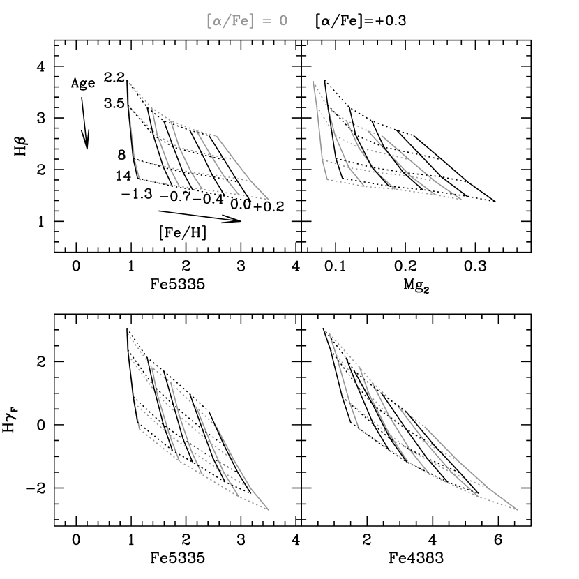
Figure 17.— Figure 16 continued. Upper Left: The Fe5335 index is shown to be only very mildly sensitive to $\alpha$-enhancement, only for high [Fe/H]. Upper Right: As expected, Mg₂ is very sensitive to [Mg/Fe], but not as strongly as Mg $b$. Lower Left: The $H\gamma_{F}$ index shows some sensitivity to $\alpha$-enhancement, mostly because of the decreased strength of CN lines, due to enhanced oxygen abundances. Lower Right: The Fe4383 index is mildly sensitive to $\alpha$-enhancement, being weaker for higher $\alpha$-element abundance, mostly due to the presence of magnesium and calcium lines in the index pseudo-continua.

In the upper right panels of Figures 16 and 17, the models are compared in the Mg $b$-$H\beta$ and Mg₂-$H\beta$ planes, respectively. One can see that the Mg $b$ and Mg₂ indices are very strongly sensitive to [Mg/Fe], as expected, with Mg $b$ being a little more sensitive than Mg₂. For this reason, these indices have been used in the literature as the chief $\alpha$-enhancement indicators. For reasons that will be discussed in Section 5.2.2, we will adopt Mg $b$ as our main indicator of magnesium abundance.

The lower left panels of Figures 16 and 17 illustrate how the Balmer line indices $H\delta_{F}$ and $H\gamma_{F}$, respectively, respond to variations of $\alpha$-element abundances. In both cases, a mild response to $\alpha$-enhancement is seen, in the sense that the indices tend to be stronger for higher $\alpha$-element abundances, so that non-consideration of $\alpha$-enhancement effects could lead to age underestimates. The effect would be of the order of 4-5 Gyr for old ages and solar metallicity, and about 1 Gyr for ages around 2 Gyr, for a stellar population with [$\alpha$/Fe] $\sim$ +0.3. While in the case of the $H\delta$ indices this is, according to Korn et al. (2005), due to contamination of the index passbands by magnesium and silicon lines (though we failed to find any of the former in the Moore et al. 1966 catalogue), in the case of $H\gamma$ it is because of the weakening of CH lines in the index pseudo-continuum, due to enhanced oxygen abundances.

The lower right panel of Figure 16 shows a comparison of solar-scaled and $\alpha$-enhanced models in the Ca4227-$H\delta_{F}$ plane. This plot shows that the Ca4227 is very strongly sensitive to [Ca/Fe], so that it will be used here as our chief indicator of calcium abundances. However, as we pointed out in the previous subsection, this index is also very heavily influenced by carbon abundance, which needs to be accounted for if one wants to use the Ca4227 index for calcium abundance determinations. Finally, the lower right panel of Figure 17 compares solar-scaled and $\alpha$-enhanced models in the Fe4383-$H\gamma_{F}$ plane. This plot suggests that Fe4383 is mildly sensitive to $\alpha$-enhancement, in the sense that it is weaker in $\alpha$-enhanced models. This results from contamination of one of the index’s pseudo-continua by Mg lines.

The main conclusions of our investigation of the effects of $\alpha$-enhancement on the Lick indices studied in this work can be summarized as follows. Amongst the Balmer line indices, $H\beta$ is the only one that is not affected by $\alpha$-enhancement, or any other abundance-ratio effects. $H\gamma_{F}$, $H\gamma_{A}$, $H\delta_{F}$, and $H\delta_{A}$ are similarly affected in the sense that they are stronger in spectra of $\alpha$-enhanced stellar populations, for fixed age and [Fe/H]. Amongst the metal lines, the Fe5270, and Fe5335 indices are essentially insensitive to $\alpha$-enhancement, Fe4383 is only mildly affected by it, and Fe5015 is strongly affected by it. This is good news, telling us that a safe estimate of [Fe/H] is warranted. Our main indicators of $\alpha$-element abundances are Mg $b$, Mg₂, and Ca4227. While Mg $b$ is our cleanest indicator of an $\alpha$-element abundance (magnesium, in this case), Ca4227 can be used to estimate calcium, provided that carbon and nitrogen abundances are known, so that the CN effect on Ca4227 can be accounted for. The abundances of carbon and nitrogen can be inferred from the combined use of either G4300 or C₂4668 (both sensitive to carbon only, but C₂4668 is preferable, see Graves & Schiavon 2006, in preparation, for a discussion) and CN₁ and CN₂ indices (sensitive to carbon and nitrogen).

4.4. A Method for Determining Mean Ages and Metal Abundances of Stellar Populations

The understanding acquired in the last Section of the response of line indices to variations of age and elemental abundances can be used to establish a method to estimate both the age and abundance pattern of stars in clusters and galaxies, from the interpretation of Lick indices measured in their integrated spectra.

Initially let us suppose that measurements for all the line indices modelled in this work are available for a given stellar system. The method consists in constraining first the most influential parameters (i.e., those which affect the largest number of observables) and then descend hierarchically towards constraining less influential parameters. Inspection of Figures 14 through 17 tells us that the parameters that affect the largest number of Lick indices are age and metallicity, which in our models is cast in terms of [Fe/H]. Virtually all the Lick indices are affected by age and [Fe/H] variations, to various degrees. Therefore, the starting point of the method is the determination of age and [Fe/H]. According to our conclusions from Section 4.3.2, the best way of estimating age and [Fe/H] is by comparing data with models in a diagram involving an iron index (preferably Fe5270 or Fe5335, or some combination of these) and $H\beta$. Therefore, we assume that the Fe and $H\beta$ indices are only sensitive to [Fe/H] and age and estimate those parameters on the basis of solar-scaled models (the choice of models here is unimportant, provided our assumption that these indices are unaffected by abundance ratios is approximately correct). The second most influential parameter is the abundance of carbon, which affects a large number of line indices, though not all of them (for instance, $H\beta$, Fe5270, and Fe5335 are essentially not affected by carbon abundances), via the contamination of index pseudo-continua and passbands by lines due to CN, CH, or C₂, which pervade the spectral region under study. Of all the indices modelled in this paper, the C₂4668 index is best suited for carbon abundance determinations, so the next step in our method consists of searching the [C/Fe] value that best matches the $C_{2}$4668 index for the same age and [Fe/H] as estimated from the analysis of $H\beta$ and Fe indices. Once [C/Fe] is estimated, the next step consists of determining [N/Fe], as the abundance of nitrogen affects a large number of indices, because of its influence on the strength of CN lines. The best indicator of nitrogen abundances are the CN bands themselves, so the next step in the procedure consists of searching the [N/Fe] value for which the CN₁ and/or CN₂ indices are matched for the same age, [Fe/H], and [C/Fe] that match the measurements of $H\beta$, C₂4668 and Fe indices. The remaining parameters in the hierarchical sequence would be [Mg/Fe] and [Ca/Fe], as they influence only a very few line indices, such as Mg $b$, Mg₂, and Ca4227. Therefore, the final step of our procedure consists of estimating [Mg/Fe] and [Ca/Fe] by searching the values that match Mg $b$/Mg₂ and Ca4227, respectively, for the same age, [Fe/H], [C/Fe], and [N/Fe] as estimated from the match to all the previous indices. Once the latter is achieved, a first estimate of age, [Fe/H], [C/Fe], [N/Fe], [Mg/Fe], and [Ca/Fe] has been reached. The process now needs to be iterated, given that we initially supposed that $H\beta$ and the Fe index/indices of choice were essentially independent of any parameters other than age and [Fe/H], which is not entirely correct. Experience shows that, for most applications and depending on the degree of internal consistency aimed, one iteration is good enough.

Table 10Cluster Parameters

Cluster ID	Age (Gyr)	[Fe/H]	[O/Fe]	[N/Fe]a	[C/Fe]a	[Mg/Fe]	[Ca/Fe]	[Ti/Fe]	[Na/Fe]	[Si/Fe]
M 5 (catalog M5)	11	–1.3$\pm$0.1	+0.3$\pm$0.2	+1.2/0.0	–1.0/–0.3	+0.3$\pm$0.1	+0.3$\pm$0.1	+0.2$\pm$0.1
47 Tuc (catalog 47 Tuc)	12	–0.7$\pm$0.05	+0.5$\pm$0.1	+1.1/+0.3	–0.2/0.0	+0.4$\pm$0.1	+0.2$\pm$0.1	+0.3$\pm$0.1	+0.2$\pm$0.1	+0.3$\pm$0.1
NGC 6528 (catalog NGC6528)b	11	–0.15/+0.1	+0.15/+0.07			+0.07/+0.14	–0.40/+0.23	–0.10/+0.23	+0.43/+0.40	+0.08/+0.36
M 67 (catalog M67)	3.5	0.0$\pm$0.1	0.0$\pm$0.1	0.0$\pm$0.1	0.0$\pm$0.1	0.0$\pm$0.1	0.0$\pm$0.1	0.0$\pm$0.1	+0.2$\pm$0.1	+0.1$\pm$0.1

4.4.1 Caveats

Two important caveats are worthy of mention. First of all, one of the single most important parameters influencing the integrated properties of stellar populations has been left out of the procedure outlined above: the abundance of oxygen. Oxygen abundances affect the stars’ interior opacities, thus having a strong impact on their structure and evolution. In our case, the abundance of oxygen therefore affects the choice of theoretical isochrones adopted in the model synthesis. Unfortunately, oxygen abundances for non-resolved, old and intermediate-age, stellar populations are unknown and very difficult to constrain. It has become standard practice in the literature to address this problem by adopting not only the assumption that oxygen tracks magnesium, but also the more far-reaching corollary that [Z/H] can be determined once Fe and Mg indices (or a combination therefrom) are matched by the models. The former, more fundamental, assumption, while grounded on the theoretical expectation that magnesium and oxygen have a similar nucleosynthetic origin (e.g., Matteucci & Tornambé 1987, Wheeler et al. 1989, Woosley & Weaver 1995) has recently been challenged by the finding that metal-rich Galactic bulge stars, which have strongly super-solar [Mg/Fe], appear to have [O/Fe] below or around solar (Fulbright, Rich & McWilliam 2005, Cunha & Smith 2006). Therefore, we emphasize that, while the assumption of oxygen tracking magnesium might be, if not entirely reasonable, the only possible way out of this quandary, it is no more than an assumption, which still awaits confirmation from a compelling observational result. For the time being, any results coming from the method proposed here should be taken with caution. A good way of dealing with this uncertainty would be to adopt two widely different values of [O/Fe] and carrying out the procedure to the end, so that the final impact of an [O/Fe] assumption on the final results can be assessed.

Another important caveat regards the uncertainties in the outputs of this method. Except for age and [Fe/H], error propagation should lead to very large error bars in the abundances of the elements at the bottom of the hierarchy devised above. Therefore, the uncertainty in the abundance of calcium, for instance, should be the highest, as the Ca4227 index is strongly influenced by the abundances of carbon and nitrogen, whose uncertainties in turn depend on the uncertainties in [Fe/H] and age. The case of magnesium is less serious, as the Mg $b$ index is strongly affected only by age, [Fe/H], besides the output parameter, [Mg/Fe]. Nitrogen stands in between those two cases, as the CN band is affected by age, [Fe/H], and [C/Fe], besides [N/Fe]. In view of these difficulties, we strongly recommend the reader to restrict application of this method to only very high S/N data, so as to prevent the very large uncertainties inherent to the method from rendering the results meaningless.

This method has been implemented by G. Graves, from Lick Observatory, as an IDL routine which will soon be made available publicly. The routine, called “EZ_Ages”, and the mathematical algorithm used to search the best solutions for a given set of index measurements are described in detail in Graves & Schiavon (2006, in preparation).

5. Comparison with Cluster Data

A fundamental test to which every stellar population synthesis model must be submitted is the comparison to Galactic clusters. If the models cannot reproduce the data for these well-known resolved systems, using the right set of input parameters, their application to galaxy evolution can be rightly called into question. It is not surprising, therefore, that there is a vast literature dedicated to such comparisons (e.g., Rose 1994, Bruzual et al. 1997, Schiavon & Barbuy 1999, Gibson et al. 1999, Vazdekis et al. 2001, Schiavon et al. (2002a,b), Maraston et al. 2003, Schiavon et al. 2004b, Proctor et al. 2004, Schiavon et al. (2004a,b), Lee & Worthey 2005, Lilly & Fritze-v. Alvensleben 2006, and references therein). In this section, we show that our models match the data of four well-known Galactic clusters to high accuracy. Our discussion is focussed on a few well known representative clusters for which very high quality CMD data and abundance analyses of cluster members are available in the literature. The absorption line indices for our globular clusters of choice were measured in the very high S/N integrated spectra collected by Schiavon et al. (2005) and, in the case of M 67, they were taken from Paper III and converted to our system of equivalent widths (but see Section 5.1). While essentially all results presented here are valid for the entire sample of 40 globular clusters observed by Schiavon et al. (2005), we defer an in-depth discussion of the whole sample to a forthcoming paper.

The clusters examined here are M 5 (=NGC 5904), 47 Tuc (=NGC 104), NGC 6528, and M 67 (=NGC 2682). Relevant data for these clusters are summarized in Table 10. Ages come from analyses of CMD data by Salaris & Weiss (2002, M 5), Paper II (47 Tuc), Ortolani et al. (2001, NGC 6528), and Paper III (M 67). The iron abundance for M 67 comes from the compilation in Paper III. Abundances for M 5 come from Cohen, Briley & Stetson (2002, [C/Fe] and [N/Fe]) and Ramírez & Cohen (2003, other ratios). Carbon and nitrogen abundances for 47 Tuc stars come from Briley et al. (2004), while for other elements abundances come from Carretta et al. (2004) and Alves-Brito et al. (2005). Oxygen abundances in 47 Tuc dwarfs come from Carretta et al. (2005). Abundances for NGC 6528 are averages of the determinations by Carretta et al. (2001), Zoccali et al. (2004), and Origlia, Valenti & Rich (2005) (but see discussion below and in Section 5.3). Regarding the abundances of carbon and nitrogen, we note that stars in M 5 and 47 Tuc (and perhaps in all globular clusters) are known to present a bimodal distribution of the abundances of these elements (e.g., Dickens, Bell & Gustafsson 1979, Norris & Freeman 1979, Smith, Bell & Hesser 1989, Cannon et al. 1998, Cohen et al. 2002, Briley et al. 2004, Carretta et al. 2005, Lee 2005, Smith & Briley 2006). For these elements, we list the extremes of the range of values spanned by cluster main sequence stars. Unfortunately, no such study is available for the C and N abundances of main sequence stars in NGC 6528. Origlia, Valenti & Rich (2005) determined carbon abundances in four bright NGC 6528 giants, reporting [C/Fe]=–0.4. This value probably reflects the workings of internal mixing, and we choose not to consider it. For M 67, the abundance ratios were taken from the compilation in Paper III, except for oxygen, calcium and titanium, which were taken from Tautvaisiene et al. (2000) and Shetrone & Sandquist (2000). Finally, because different groups disagree as to the metal abundances of NGC 6528 (Carretta et al. 2001, Barbuy et al. 2004, Zoccali et al. 2004), abundances by these two different groups are listed for this cluster. This issue is further discussed in Section 5.3.

Figure 18.— Data on M 67 (star) and NGC 6528 (filled square) compared to solar-scaled model predictions. Same-age models are connected by dotted lines, except for the 3.5 Gyr models, which are connected by dashed lines, for clarity. Same-[Fe/H] lines are solid. The ages of the models displayed are, from top to bottom, 1.2 (barely visible), 1.5, 2.5, 3.5, 7.9, and 14.1 Gyr. The values for [Fe/H] are, from left to right, –0.7, –0.4, 0.0, and +0.2. The best-fitting model for M 67 has an age of $\sim$ 3.8 Gyr and [Fe/H]=–0.08. Note the consistency with which all indices are matched by the models at essentially the same position on the grid.

Comparison of the data on elemental abundances shown in Tables 6 and 10 suggests that the overall abundance pattern of the cluster stars is mostly quite similar (to within 0.1 dex) to that of our library stars with the same [Fe/H]. In fact, in the case of M 67 there is an almost perfect match between cluster and field star abundance patterns. For the globular clusters, though, there are a few important exceptions that need to be kept in mind. The relative abundances of carbon and nitrogen in globular-cluster stars deviate strongly from those of field stars. The main consequence is that, in integrated light, globular clusters tend to show strongly enhanced CN lines and slightly weaker CH lines when compared to models based on spectra of field stars (see Paper I for a detailed discussion). This should mainly affect the comparison of our model predictions to data on the CN₁, CN₂, G4300, and C₂4668 indices but can also disturb other indices whose passband and/or pseudo-continua contain lines due to these molecules (for instance, Ca4227, see below, or the $H\gamma$ indices). Another important difference is the one between the abundance pattern of NGC 6528 and that of library stars of near-solar metallicity. This bulge cluster has higher [O/Fe] by $\sim$ 0.1 dex and [Ca/Fe] (potentially) lower by $\sim$ 0.4 than field stars of the same metallicity. Its relative magnesium abundance seems to be slightly higher as well. These few exceptions aside, it is fair to say that the abundance patterns of the clusters and the field stars employed in our model construction are a relatively good match. Therefore, we first compare our base-model predictions with cluster data without performing any correction to bring the models into the cluster abundance pattern (except in the case of M 67, for which such comparisons were discussed in Paper III and will not be repeated here). Confrontation between cluster data and models tuned to the clusters abundance patterns are discussed in Sections 5.2.3 and 5.3.

5.1. M 67

Figure 19.— Figure 18 continued. Model age and [Fe/H] are the same as in Figure 18. Note the outstanding consistency with which all the indices from M 67 are matched by the models (i.e., same age and [Fe/H] everywhere). Due to a spectral blemish in the Schiavon et al. (2005) data, the Fe5015 is not available for NGC 6528.

The open cluster M 67 has an age of $\sim$ 3.5${}^{+1.0}_{-0.5}$ Gyr and nearly solar metallicity ([Fe/H] = 0.0 $\pm$ 0.1). Therefore, it inhabits a region of parameter space that is very important for studies of the integrated light of galaxies, both nearby and at large distances, where early-type galaxies are often found to have similar mean ages and metallicities (e.g., Trager et al. 2000, Kelson et al. 2001, Caldwell et al. 2003, Denicoló et al. 2005a,b, Gallazzi et al. 2005, Schiavon et al. 2006).

5.1.1 The Integrated Spectrum of M 67

In Paper III an integrated spectrum of M 67 was obtained from coaddition of individual spectra of cluster members, weighted according to their luminosities and relative numbers, assuming a Salpeter IMF. Since publication of that work a few revisions have been made to the cluster integrated spectrum and Lick indices measured in it, so that an update on these observables is made necessary here. The first important change relative to the values published in Paper III refers to the EW measurements, which had to be retaken, for the reasons exposed in Section 2.2. The second important revision relates to star #6472 (ID from Montgomery, Marschall & Janes 1993), which has been erroneously included in the coaddition as a first-ascent giant star. Inspection of Figure 1 in Paper III suggests that this star is too blue (by $\mathrel{\hbox{\raise 2.15277pt\hbox{$>$}\hbox to0.0pt{\hss\lower 2.15277pt\hbox{$\sim$}}}}$ 0.2 mag in B–V) to be on the red giant branch of M 67, which is confirmed by its warm spectrum. It is also too bright and too blue to be an early-AGB star. Because of its uncertain evolutionary stage, we decided to remove this star from the coaddition to produce the cluster integrated spectrum. In the third relevant change, we performed a test which showed that main sequence M 67 stars fainter than V $\sim$ 15 (the magnitude limit in Paper III sample) contribute significantly to the integrated Lick indices of the cluster. In order to correct for this effect, we used the Padova isochrones that best matched the cluster color-magnitude diagram (Girardi et al. 2000, solar-scaled, solar metallicity, 3.5 Gyr-old) to compute model predictions including and excluding stars less massive than $\sim$ 0.85 $M_{\odot}$. The difference between these two model predictions was used to correct the Lick indices measured in the cluster integrated spectrum for the contribution of low-mass stars. Both corrected and uncorrected Lick indices for M 67 are listed in Table 11. Comparison between the two sets of indices shows the corrections are small, but not negligible for some indices. These numbers supersede the values provided in Paper III and will be used throughout this paper in our comparison with model predictions.

Table 11Revised Lick Indices for M 67

	$H\delta_{F}$	$H\delta_{A}$	CN1	CN2	Ca4227	G4300	$H\gamma_{F}$	$H\gamma_{A}$	Fe4383	C24668	$H\beta$	Fe5015	Mg2	Mgb	Fe5270	Fe5335
M67	1.0	–0.1	–0.005	0.019	0.82	4.7	–0.21	–4.0	3.8	4.5	2.4	4.7	0.161	2.8	2.6	2.2
M67–Corr1	1.0	–0.3	–0.007	0.018	0.93	4.7	–0.32	–4.2	3.8	4.4	2.2	4.7	0.175	2.9	2.6	2.3
Error	0.1	0.2	0.006	0.007	0.08	0.1	0.07	0.2	0.2	0.1	0.1	0.4	0.006	0.2	0.1	0.1

5.1.2 Confronting Models with M 67 Data

Figure 20.— Figure 18 continued, now showing comparisons between models and data for indicators of carbon, nitrogen, and magnesium abundances. Again, data for M 67 are matched consistently for the same age and [Fe/H] as for indices in the previous figures.

In Paper III we presented a detailed comparison between our solar-scaled models and Lick indices for M 67. We showed that our models match the Balmer line indices $H\beta$, $H\gamma_{F}$, and $H\delta_{F}$ for the same age that is inferred from the fit of the cluster’s color-magnitude diagram, to within $\sim$ 0.5 Gyr. Moreover, we showed that the indices $<Fe>$ (the average of indices Fe5270 and Fe5335), Mg $b$, CN₁, and CN₂ were matched for the known cluster elemental abundances to within $\pm$ 0.1 dex. Here we extend these comparisons to include the remaining indices modelled in this paper. In order to find the model that best matches the data for M 67, we applied the method described in Section 4.4 and found the following best-fitting parameters, using the Padova solar-scaled isochrones and assuming solar [O/Fe]: age $\sim$ 3.8 Gyr, [Fe/H]=–0.08, [Mg/Fe]=0.01, [C/Fe]=–0.03, [N/Fe]=+0.02, and [Ca/Fe]=–0.03. The models computed for this abundance pattern are provided in Table A6 in the Appendix. Inspection of Table 10 shows that these results agree with the known cluster values to within 0.3 Gyr and 0.08 dex in age and metal abundances, respectively. In Figures 18 through 21 these best-fitting models are compared with Lick indices for M 67 in a number of relevant index-index diagrams. The model ages and metallicities plotted are as follows: 1.2, 1.5, 2.5, 3.5, 7.9, and 14.1 Gyr, and [Fe/H] = –0.7, –0.4, 0.0, and +0.2. The filled squares represent data for NGC 6528, which will be discussed in Section 5.3.

Figure 21.— Figure 18 continued, now showing comparisons between models and data for indices sensitive to iron, calcium and carbon. The G4300 index is the one for which the models are the poorest match to the data (almost 0.2 dex too metal-rich, according to the models).

Figures 18 and 19 compare data to models in metal vs. age-sensitive-index plots. For almost all indices, the data for M 67 fall within 1-$\sigma$ of our model prediction for a solar-metallicity, 3.5 Gyr-old, single stellar population. In Figures 20 and 21 the data for indices sensitive to carbon, nitrogen, magnesium, and calcium are compared with the models, using $H\beta$ as age indicator. Again, the models are a satisfactory match to the data for the correct age and metal abundances. We call attention for the very good match obtained for Ca4227, which was not discussed in Paper III. We note that in that paper we could not match the M 67 data for G4300. The match here is slightly improved, though still not entirely satisfactory. The G4300 index is matched for a model with [Fe/H]$\sim$+0.1, which is almost 0.2 dex too metal-rich compared with the value obtained from the match to the C₂4668 index, which is in much better agreement with the cluster known carbon abundance. This result should serve as a warning against use of the G4300 index for carbon abundance determinations in metal-rich stellar populations (see Graves & Schiavon 2006, in preparation).

In summary, the models match the age of M 67 and its abundances of iron, carbon, nitrogen, magnesium and calcium to within 1 Gyr and 0.1 dex. Most importantly, the ages according to all Balmer line indices are consistent to within 0.5 Gyr. This is a very encouraging result that ratifies the application of our models for estimation of mean ages and metal abundances of stellar systems in a very important age/metallicity regime. To some extent, this is not surprising, given that the integrated light of the cluster over most of the spectral interval involved in this study is dominated by turnoff stars which, in the case of M 67, are characterized by mid-F spectral types of solar metallicity, for which most of the physical input and calibrations underlying the models are very well established. The fact that the abundance pattern of our models for solar metallicity are a close match to that of the cluster is also very helpful. In the next sections we focus on the more challenging task of matching the data for Galactic globular clusters, which depart considerably from the regime where such favorable conditions are enjoyed.

5.2. 47 Tuc and M 5

Figure 22.— a. Data for M 5 (left) and 47 Tuc. The arrow indicates how the predictions for M 5 change when the contribution due to blue HB stars is “removed” from the cluster data. Ages are 1.2, 1.5, 2.5, 3.5, 7.9, and 14.1 Gyr, and metallicities are [Fe/H]=–1.3, –0.7, –0.4, 0.0, and +0.2. The models for 3.5 Gyr are connected by a dashed line, to guide the eye. The models for [Fe/H]=–1.3 are not shown in Figure 22e. See detailed discussion in the text.

In this Section, we compare our model predictions to data for two of the best studied Galactic globular clusters, 47 Tuc and M 5. It is very interesting to test our models in the region of stellar population parameter space occupied by metal-poor to mildly metal-rich old globular clusters, in view of the on-going efforts to constrain the history of merging/star-formation of external galaxies through the determination of the spectroscopic ages and metallicities of their globular clusters (e.g., Cohen et al. 1998, Cohen, Blakeslee & Côté 2003, Larsen et al. 2003, Burstein et al. 2004, Beasley et al. 2005, Puzia et al. 2005, Brodie & Strader 2006, and references therein).

The data for these two clusters are compared to the models in Figures 22a through 22f. The abundance patterns of 47 Tuc and M 5 are $\alpha$-enhanced (Table 10), in particular with [O/Fe] = +0.5 and +0.3, respectively. We recall from Section 4.3.1 that the $\alpha$-enhanced Padova isochrones were computed assuming [O/Fe]=+0.5. However, they do not extend to low enough metallicities for a comparison with M 5 data. Moreover, Weiss et al. (2006) showed that the Padova $\alpha$-enhanced isochrones need to be revised (see discussion in Section 4.3.1) so that we choose to compare the data with models generated using the solar-scaled Padova isochrones (models 1–5 in Table 9). This set of theoretical isochrones does not match the oxygen abundances of the two clusters. However, based on our discussion in Section 4.3.1, the evolutionary $\alpha$-enhancement effects are well-understood, so that we can use models based on solar-scaled isochrones, while keeping in mind the effect of that inconsistency. In particular, we expect to predict slightly too old ages, regardless of the Balmer line used.

5.2.1 Fe vs Balmer Lines

Figure 22.— b.

As in the previous Section, we first focus on plots between Fe and Balmer lines, because these indices are mostly sensitive to age and [Fe/H] (see discussion in Section 4.3.2). We first consider the case of 47 Tuc. In all the panels in Figures 22a through 22c the models predict the correct [Fe/H] of the cluster to within $\pm$ 0.05 dex. The spectroscopic age for this cluster according to the models is $\sim$ 14 Gyr, which is older by $\sim$ 2–3 Gyr than the age based on analysis of the cluster CMD using the $\alpha$-enhanced Padova isochrones (Paper II). Roughly half of this mismatch is due to our adoption of solar-scaled isochrones in the current calculation. The rest of the discrepancy is due to an effect pointed out in Paper II, where it was shown that it is motivated by a mismatch between the observed luminosity function of the cluster and theoretical predictions, which underestimate the number of giant stars brighter than the horizontal branch (HB), relative to main sequence stars. While it is not clear whether this mismatch between data and theory in the luminosity function space is restricted to 47 Tuc and a few other clusters (e.g., Langer, Bolte & Sandquist 2000) Zoccali & Piotto (2000) found an apparent trend according to which models seem to under-predict the relative number of giants in more metal-rich clusters. Zoccali & Piotto point out that uncertainties in the bolometric corrections for metal-rich cool giants might be responsible for the mismatch, but to our knowledge this hypothesis has not yet been tested. Clearly, more work is needed to clarify this matter.

The case of M 5 is very interesting. The Balmer lines in this cluster’s spectrum are too strong for its age. In Figures 22a through 22c, the spectroscopic age of M 5 according to the models is somewhere between 4 and 6 Gyr (probably even a little younger, if the [Fe/H]=–1.3 models were based on $\alpha$-enhanced isochrones). This is in stark contrast with the known CMD-based age of the cluster ($\sim$ 11 Gyr). This effect has been pointed out before (Freitas Pacheco & Barbuy 1995, Lee, Yoon & Lee 2000, Maraston & Thomas 2000, Schiavon et al. 2004b) and is due to the influence of blue HB stars which are not accounted for by the theoretical isochrones adopted in our models. These old and bright A-F-type stars have very strong Balmer lines which can mimic a young turnoff if not properly accounted for by the models. Schiavon et al. (2004b) studied this problem and devised a method to disentangle this degeneracy between age and HB-morphology, which explores the differential sensitivity of $H\delta$ and $H\beta$ to the influence of blue HB stars.

Figure 22.— c.

The theoretical isochrones adopted in our models do not produce blue HB stars in the metallicity range considered here. The morphology of the HB is chiefly dictated by mass loss along the giant branch phase, a phenomenon for which a deterministic theory is still lacking. As a result, models for the mass loss along the giant branch rely on empirical calibrations of mass-loss rates as a function of stellar parameters, thus having limited predictive power. Therefore, we adopt a more conservative path and just correct the observations of M 5 for the effect of blue HB stars, on the basis of a high-quality CMD for the cluster (see details in Schiavon et al. 2004b). In this way we can at least check whether our models predict correctly the cluster properties in the absence of blue HB stars. The arrows attached to the data for M 5 indicate how the line indices change when the contribution from blue HB stars is removed. These arrows were computed by Schiavon et al. (2004b), from a combination of the color-magnitude diagram of M 5 (from Piotto et al. 2002) and the fitting functions presented here. For details, see Schiavon et al. (2004b). In all panels of Figures 22a–c we can see that the age predicted by the models for the HB-free version of M 5 is $\sim$ 10 Gyr and [Fe/H] $\sim$ –1.3, in outstanding agreement with the values listed in Table 10. Given the uncertainties involved in the model calibrations at the low metallicity end and in the correction for the effects of blue HB stars, we consider this a very satisfactory result.

Figure 22.— d.

5.2.2 Light-element Indices vs Balmer Lines

Figure 22.— e.

In Figures 22d–f we show the cluster data compared with the models in light-element-index vs Balmer-line planes. We first focus on the case of the the indices Mg₂ and Mg $b$, which are mostly sensitive to the abundance of magnesium. In the case of Mg $b$, the agreement between models and data is very good, especially for 47 Tuc, for which the 14 Gyr-old model for [Fe/H]=–0.7 falls right on top of the data points in all three panels. This is not surprising, given that [Mg/Fe] for both the models and the cluster (Tables 6 and  10) differ by only $\sim$ 0.1 dex. The same is not true for Mg₂, for which the model for the same age and metallicity is too strong by 0.03 mag, which would lead to an underestimate of roughly 0.3 dex in [Mg/H]. We suggest that this mismatch is due to the extreme mass segregation in the cluster cores. Because the core of 47 Tuc is strongly depleted of low-mass stars (e.g., De Marchi & Paresce 1995, Howell et al. 2001, Monkman et al. 2006), Mg₂ tends to be weaker than the value predicted for a Salpeter IMF, while Mg $b$, which is not so sensitive to the contribution by low mass stars, is less affected (see discussion in Section 4.2). The most recent determination of the mass function in the core of 47 Tuc was performed by Guhathakurta et al. (2006, in preparation, but see Monkman et al. 2006), who found that, within the cluster core, the mass function below the turn-off is well matched by a power law with $x\sim-4.0$. In Figure 23 we illustrate the effect of mass segregation by comparing calculations performed with a Salpeter IMF ($x=1.35$, bottom panels) and a dwarf-depleted mass function ($x=-4.0$). It can be seen that dwarf-depleted match Mg₂ considerably better than those based on a Salpeter IMF. The predictions for Mg $b$ change very little in comparison, with the models agreeing with the data to within 0.1 ${\rm\AA}$. Because both indices are subject to the influence of elemental abundances that may be somewhat uncertain, we only suggest that the initial inconsistency between the magnesium abundances based on Mg $b$ and Mg₂ might be due to mass segregation effects. In any case, the conclusion that a combination of these two indices can be used to constrain the low-mass end of the mass function is robust, provided other variables such as abundance ratios are tightly constrained.

Figure 22.— f.

We note that in Figure 23 the dwarf-depleted models have slightly stronger $H\beta$ than those computed with a Salpeter IMF. This can be understood in terms of the relative contribution to the integrated light at $\sim$ 4861 ${\rm\AA}$ by giant, turnoff, and lower main sequence stars. Comparing the numbers for dwarf-depleted and Salpeter-IMF models one finds that, because the initial masses of turnoff and giant stars are essentially the same, the (giant-to-dwarf) ratio between the contribution by these two types of stars to the integrated light varies only by a factor of 1.5 between the two models (being of course higher in dwarf-depleted models). On the other hand, the ratio between giants and lower main-sequence stars varies by roughly a factor of 6. Because giants have stronger $H\beta$ than lower main-sequence stars, the net result is that dwarf-depleted models have stronger $H\beta$. Of more interest to us is the fact that the dwarf-depleted models over-predict the value of $H\beta$ in 47 Tuc by $\sim$ 0.2 ${\rm\AA}$, so that the spectroscopic age of the cluster according to those models is a bit too old. This is not unexpected. As we mentioned in Section 5.2, the oxygen abundance of 47 Tuc is much higher than that adopted in the models of Figure 23. The effect of adopting the right oxygen abundance for 47 Tuc can be gauged by comparing the thick lines in Figure 23, which correspond to computations performed adopting the $\alpha$-enhanced Padova isochrones, for which [O/Fe]=+0.5. While agreement with $H\beta$ in 47 Tuc is improved, the discrepancy is not entirely removed. This is because, as discussed in Section 4.3.1, the $\alpha$-enhanced Padova isochrones overpredict the temperatures of turn-off and giant stars, as pointed out by Weiss et al. (2006). In Section 4.3.1, we estimated an approximate correction to our model predictions and found that $H\beta$ in old $\alpha$-enhanced models should be weaker by roughly 0.15 ${\rm\AA}$, which would bring our models into very good agreement with 47 Tuc data.

Figure 23.— Effects of mass function on the predictions for the Mg indices. Upper panels: a dwarf-depleted IMF is adopted, consistent with the clusters’ heavy mass-segregation. Lower panels: Same as the top panels of Figure 22d, where a Salpeter IMF is adopted in the computations. Note the improved agreement between model and data for Mg₂ in the upper panels.

In Figure 22e the data are compared in CN-index vs Balmer-line planes. It can be seen that the clusters have much stronger CN indices than predicted by the models. In the case of 47 Tuc, CN₁ (CN₂) is stronger by 0.06 (0.08) mag than the model for [Fe/H]=–0.7 and 14 Gyr, so that in all panels the cluster falls near the solar metallicity locus. This is not a new result (e.g., Vazdekis 1999, Paper I, Puzia et al. 2002) neither is it unexpected. As anticipated in the beginning of Section 5, the relative abundances of carbon and nitrogen of models and cluster are largely discrepant (Tables 6 and 10). In Figure 22f, model predictions for C₂4668 and Ca4227 are compared with the data. Interestingly, models overpredict the values of both indices. In the case of C₂4668, this probably indicates that the mean luminosity-weighted [C/Fe] is below solar, which is not surprising, given the abundances measured in individual stars (Table 10). The case of Ca4227 is interesting. Despite the fact that the relative abundance of calcium in the models is a very close match to that of the clusters, there is a very large mismatch with the data. In the case of 47 Tuc, the 14 Gyr-old, [Fe/H]=–0.7 model over-predicts Ca4227 by $\sim$ 0.6 ${\rm\AA}$, leading to an underestimate in [Ca/H] by more than 0.7 dex. We suspect that this might in part be due to the influence of CN lines on the Ca4227 index. These results clearly indicate that indices sensitive to carbon and nitrogen abundances need to be corrected for abundance-ratio effects. This is the topic of Section 5.2.3.

5.2.3 CN-Strong Models for Globular Clusters

We have seen in the previous section that the base models do an excellent job of reproducing the Balmer, Fe, and Mg indices for one metal-poor and one mildly metal-rich Galactic globular cluster. The same level of agreement was not reached, however, for the carbon, nitrogen and calcium-sensitive indices. In order to address this problem we computed a new set of models adopting the known abundance pattern of 47 Tuc, following the procedure outlined in Section 4.3.2, so as to generate CN-strong models for this cluster. Such models may be very useful given the fact that the CN-strong phenomenon in integrated spectra of globular clusters seems to be ubiquitous, being probably caused by very high nitrogen abundances (e.g., Burstein et al. 1984, Brodie & Huchra 1991, Papers I and II, Li & Burstein 2003, Beasley et al. 2004, Burstein et al. 2004).

The elemental abundances adopted for 47 Tuc are those listed in Table 10. Because carbon and nitrogen have a bimodal distribution, we computed two sets of models, corresponding to the CN-strong and CN-weak abundance patterns. These models were then combined, with weights determined by the relative numbers of CN-strong and CN-weak stars in the core of 47 Tuc, from Briley (1997), who found CN-strong/CN-weak $\sim$ 2. In view of the mass-segregation effects discussed in the previous section, we adopted a dwarf-poor IMF in these computations, with x=–4 (equation 3).

In Figure 24 these models are compared with our base models (1-5 in Table 9, in a few interesting index-index plots. Gray lines represent the base models, while dark lines represent the CN-strong models described above. Same-[Fe/H] models are connected by dotted lines. As expected, CN-strong models are characterized by stronger CN₂, and weaker carbon indices (G4300 and C₂4668). The behavior of Ca4227 is more complex. It is weaker in metal-poor models, where [Ca/Fe] and [O/Fe] in the CN-strong and base models are similar, so that the differences arise purely due to the stronger CN strengths in the former. At higher metallicities, Ca4227 becomes stronger in the CN-strong models because those have higher [Ca/Fe] and [O/Fe] than the base models, by 0.1 and 0.6 dex, respectively.

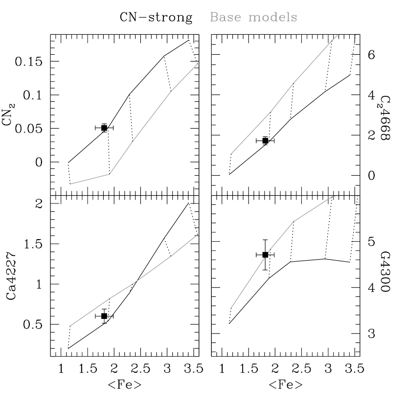
Figure 24.— Comparison, between data for 47 Tuc and models in iron vs. CN-sensitive data plots. Models shown are all for an age of 14.1 Gyr. Gray lines: base models from Table 9. Dark lines: models computed for the abundance pattern of 47 Tuc. Dotted lines connect same-[Fe/H] models (from left to right, [Fe/H]=–1.3, –0.7, –0.4, 0.0, +0.2). The models with [Fe/H]=–0.7 and the cluster abundance pattern reproduce very well all indices except for G4300. See text.

Also shown in Figure 24 are line indices in the spectrum of 47 Tuc. It can be seen that in all plots 47 Tuc is well matched by the 14 Gyr-old, CN-strong, models with [Fe/H]=–0.7 (the second dotted line from left to right), except for the case of G4300. For Ca4227, C₂4668, and CN₂ the CN-strong models are a vast improvement over CN-normal models (the same is true of CN₁, not shown). In the case of Ca4227, this result highlights an important fact, seldom appreciated in the literature: the Ca4227 index is very sensitive to the abundances of carbon and nitrogen, due to a contamination of its blue pseudo-continuum window by a CN band-head. In order to circumvent this problem, Prochaska et al. (2005) propose the definition of a new index, Ca4227r, which is far less sensitive to the CN contamination, thus being a more reliable indicator of the calcium abundances. See Prochaska et al. (2005) for details. Finally, we note that adoption of these CN-strong models only affects predictions of these carbon/nitrogen-sensitive indices, so that the quality of the match to all other indices is the same as in the previous plots. Models computed for both the CN-strong and CN-normal abundance patterns of 47 Tuc stars (Table 10) and a dwarf-depleted IMF ($x=-4$) are provided in Tables A7 and A8 in the Appendix.

5.3. NGC 6528

Figure 25.— Comparison of data for NGC 6528 with model predictions assuming the input parameters listed in Table 12. Note the consistency with which models match all indices for the same age and [Fe/H]. Ages plotted are 1.5, 2.5, 3.5 (dashed), 7.9, and 14.1 Gyr, and metallicities are [Fe/H] = –0.7, –0.4, 0.0, and +0.2.

The bulge cluster NGC 6528 is one of the most metal-rich Galactic globular clusters, with [Fe/H] determinations ranging between –0.15 and +0.1 (Carretta et al. 2001, Zoccali et al. 2004, Origlia et al. 2005). Besides, it is known to be old ($\sim$ 11 Gyr, Ortolani et al. 1995, Feltzing & Johnson 2002). The abundance pattern of NGC 6528 is still a subject of debate, as the three recent studies mentioned above quote significantly different abundances for some very important elements (Table 10). For instance, abundance determinations in these studies differ by as much as 0.2 dex in the case of iron, 0.3 dex in the case of oxygen, magnesium, and silicon, 0.4 dex for titanium, and 0.8 dex in the case of calcium. Moreover, the carbon and nitrogen abundances of main sequence stars are unknown. These uncertainties are probably due to difficulties associated to the cluster’s distance and severe reddening, which has made it so far impossible to obtain high-resolution spectra of unevolved stars, for which both the uncertainties involved in the abundance determinations and star-to-star variations are less important.

As a prelude to our effort towards matching the data on NGC 6528 with models based on the cluster abundance pattern, we show in Figures 18 through 21, the indices for NGC 6528 over-plotted on models with a nearly solar abundance pattern. The abundance pattern of these models (models 1–5 in Table 9, and Table 6) differs from that of the cluster (Table 10), so we do not expect a perfect match to the data, but the comparison might be nonetheless instructive. From these figures, it can be seen that: 1) the age of the cluster according to $H\beta$ is $\sim$ 14 Gyr, which is slightly too old, while it is a bit younger according to the $H\gamma$ and $H\delta$ indices (roughly 10 and 12 Gyr, respectively). This is not unexpected given that, while NGC 6528 stars seem to be at least slightly oxygen-enhanced, the isochrones adopted in the model computations are solar-scaled. Recall that different Balmer lines respond differently to $\alpha$-enhancement (Section 4.3) and therefore should change in different ways if we switched to $\alpha$-enhanced models. 2) The iron abundances, according to Fe4383, Fe5270, and Fe5335 range between –0.3 and –0.2 dex, in rough agreement with the lower value in Table 10; 3) relative to the models, the cluster looks too strong in the CN indices, which suggests the existence of CN-strong stars, just as in the case of 47 Tuc and M 5; 4) NGC 6528 looks mildly too strong in the Mg indices, which is consistent with its measured [Mg/Fe]; 5) as in the case of 47 Tuc and M 5, NGC 6528 is very weak in Ca4227 which, given its very strong CN indices, is hinting that the effect of CN lines on Ca4227 discussed in the case of 47 Tuc might be in operation also for NGC 6528.

Table 12Best Fitting Model for NGC 6528

Isochrone	Age	[Fe/H]	[O/Fe]	[N/Fe]	[C/Fe]	[Mg/Fe]	[Ca/Fe]	[Ti/Fe]	[Na/Fe]	[Si/Fe]
Girardi et al.	13	–0.2	+0.15	+0.5	–0.1	+0.1	–0.1	–0.1	+0.4	+0.1

Now we turn to the task of producing models that mirror the abundance pattern of NGC 6528. Ideally, we would perform an exercise similar to that of Section 5.2.3, but given the above mentioned uncertainties in the cluster elemental abundances, we have to proceed differently. Instead, we adopt the method discussed in Section 4.4 in order to search the age, metallicity, and abundance pattern that are a best match to the cluster data. We adopt solar-scaled Padova isochrones in this exercise, because they match more closely the abundance pattern of the cluster, particularly the abundance of oxygen. The $\alpha$-enhanced Padova isochrones were computed assuming [O/Fe] = +0.5, whereas the cluster, according to analyses of individual stars by Zoccali et al. and Carretta et al. has at most [O/Fe] $\sim$ +0.15. Other $\alpha$-elements, like magnesium and titanium, are roughly +0.4 dex more enhanced relative to iron in the $\alpha$-enhanced Padova isochrones, which is roughly +0.3 dex higher than measured in cluster stars. Moreover, as discussed in Section 4.3.1, Weiss et al. (2006) have shown that there is a problem with the metal-rich $\alpha$-enhanced Padova isochrones, so we refrain from adopting them in the analysis of NGC 6528. The input abundances of titanium, sodium, and silicon were taken from Zoccali et al. (2004, see Table 10).

Figure 26.— Figure 25 continued. Here the models are compared to data for indices sensitive to the abundances of calcium, carbon, nitrogen, and magnesium. Note that the best matching models have the same age and [Fe/H] as those in Figure 25 (except for G4300, which is matched for a slightly too young age—see text).

The parameters of the best-fitting model are listed in Table 12, and it is compared with cluster data in representative index-index diagrams in Figures 25 and 26 Comparing the numbers in Tables 10 and 12, one can see that the best-fitting spectroscopic age (based on $H\beta$, according to the method described in Section 4.4) is 2-Gyr older than the CMD-based age from Feltzing & Johnson (2002). While on one hand this difference is comfortably within the errors, given the error bars in both studies ($\pm$ 2 Gyr), on the other it can be traced to Feltzing & Johnson’s adoption of the $\alpha$-enhanced Padova isochrones for Z=0.04. According to Table 9, this model has [Fe/H] = 0.01 and [O/Fe] = +0.5, which are respectively $\sim$ 0.2 and 0.4 dex higher than found in this study and in spectroscopic abundance determinations of cluster stars (which mostly preceded Feltzing & Johnson’s study). Accounting for both [Fe/H] and [O/Fe] differences would bring the ages in both studies into agreement.

Consistency between age estimates based on the various Balmer line indices has also been largely achieved. Ages according to $H\gamma_{F}$, (10 Gyr), $H\delta_{F}$ (12 Gyr), and $H\gamma_{A}$ (13 Gyr, not shown) agree very well with the $H\beta$-based age. The only exception is that of $H\delta_{A}$ (not shown), according to which the spectroscopic age of the cluster is $\sim$ 8 Gyr. We recall that no such effect was seen for more metal-poor and younger clusters in Sections 5.2 and 5.1.2. Inspection of the Korn et al. (2005) tables reveals that the elemental abundance that affects $H\delta_{A}$ the most strongly (after iron) is that of silicon. If we adopt the [Si/Fe] determination by Carretta et al. (2001), which is higher than that of Zoccali et al. (2004) by $\sim$ 0.3 dex, the $H\delta_{A}$-based age becomes 10 Gyr, which is in much better agreement with the ages based on the other Balmer lines. That might also explain why no such discrepancy was found for the other clusters, for which the abundance of silicon used as input is well constrained. While this result could be construed as favoring a [Si/Fe] value at the higher end of the wide range allowed by abundance determinations from the literature, we prefer to wait for the matter to be settled by further detailed abundance studies. We therefore conclude that the Balmer line indices are indicating consistent ages for NGC 6528, the only exception being $H\delta_{A}$, which indicates mildly too young ages, possibly because the index is affected by the (poorly constrained) abundance of silicon. Finally, we note that, within the uncertainties, there is a trend of slightly younger ages towards higher-order Balmer lines. We speculate that this mismatch is partially due to the adoption of theoretical isochrones whose [O/Fe] is too low. While the Girardi et al. (2000) isochrones adopted in the mild-$\alpha$ models have [O/Fe]=0, spectroscopic determinations tell us that the cluster has at least [O/Fe] $\sim$ +0.1 and might be slightly higher. As discussed in Section 4.3.1, model predictions for $H\beta$ are substantially more affected by oxygen abundances than the higher order Balmer lines. In fact, it can be seen in Figure 12 that in the old, metal-rich, regime ($\sim$ 14 Gyr, [Fe/H] $\mathrel{\hbox{\raise 2.15277pt\hbox{$>$}\hbox to0.0pt{\hss\lower 2.15277pt\hbox{$\sim$}}}}$ 0) $H\delta_{F}$ is essentially unaffected by the oxygen abundance of the theoretical isochrones adopted. Therefore, adoption of theoretical isochrones with slightly higher [O/Fe] would decrease the $H\beta$-based ages and bring it into better agreement with those based on the higher order Balmer lines and analysis of the cluster CMD.

The best-fitting abundances of iron and magnesium are also in very good agreement with values from the literature, though in both cases our estimates fall at the low end of the range allowed by abundance determinations from the literature. We call attention for the remarkable consistency of the [Fe/H] estimates coming from Fe4383, Fe5270, and Fe5335 (Fe5015 is not available for NGC 6528), which agree with each other within 0.05 dex. Magnesium abundances according to Mg $b$ and Mg₂ differ by $\sim$ 0.2 dex, in the sense that the latter are higher. It is hard to understand the reason for this discrepancy. One possible explanation may be the existence of line opacity sources that are unaccounted in the Korn et al. (2005) sensitivity tables. A strong candidate would be the TiO molecule, which is very strong in cool giants which must be present in metal-rich systems such as NGC 6528. However, from the discussion in Section 4.2, we would expect Mg $b$ to indicate higher magnesium abundances than Mg₂, which is the opposite of what we are observing. While this issue certainly deserves further scrutiny, we believe that the Mg $b$-based abundance is more reliable, since this index is not affected by flux-calibration or IMF uncertainties (Sections 2.2 and 5.2.2, respectively).

The abundances of carbon and nitrogen in NGC 6528 stars were not determined in the studies summarized in Table 10, so that our estimates listed in Table 12 are a first attempt in that direction. We find that NGC 6528 follows a pattern that is similar to that 47 Tuc (Section 5.2), being slightly carbon-depleted and very strongly nitrogen-enhanced. It is reasonable to suppose that the same type of dichotomy in the abundances of carbon and nitrogen that is found in M 5, 47 Tuc, and many other clusters (e.g., Dickens et al. 1979 Norris & Freeman 1979, Smith et al. 1989, Cannon et al. 1998, Cohen et al. 2002, Briley et al. 2004, Carretta et al. 2005, Lee 2005, Smith & Briley 2006, and references therein) may also be present in NGC 6528, though this needs to be confirmed by spectroscopy of individual stars. We note that there is a slight disagreement between the carbon abundances obtained from matching the G4300 and C₂4668 indices, in that the latter are higher by $\sim$ 0.1 dex. While this discrepancy is minor it should be subject to further investigation in the future (Graves & Schiavon 2006, in preparation). Finally, we point out that our value for [Ca/Fe] falls within the range of abundance determinations from the literature, which is no great accomplishment, given the sizable disagreement between the estimates by the different groups. Clearly, more work is needed in this front.

We conclude that the data for NGC 6528 are very well matched for a mildly $\alpha$-enhanced abundance pattern and for an age that is in very good agreement with determinations based on analysis of the cluster color-magnitude diagram. Furthermore, we find that the cluster data are well matched for a [C/Fe]= $\sim$ –0.1 and [N/Fe] $\sim$ +0.5, which mirrors the abundance pattern of other Galactic clusters, indicating that NGC 6528 stars are liable to present similar bimodal distributions in their carbon and nitrogen abundances. We found outstanding consistency between the ages and iron abundances determined from different indices, but small discrepancies in the cases of carbon and magnesium.

The models computed for the abundance pattern given in Table 12 are provided in Table A9 in the Appendix.

5.4. Summary

We have performed a detailed comparison of our models with high quality data from a representative set of Galactic clusters. For the clusters with very well known ages, metallicities, and abundance ratios (M 67, 47 Tuc, and M 5), our models matched essentially all the line indices with a very high degree of consistency, for the right set of input parameters (even though for M 5 that was only possible once the contribution by blue horizontal branch stars to the integrated light of the cluster was removed). For NGC 6528, where the metal abundances are more uncertain and, in the case of carbon and nitrogen, unknown, we followed the procedure described in Section 4.4 in order to estimate the cluster age and metal abundances. The input parameters of the best-fitting model are well within the range allowed from previous work on stellar abundances and ages. In the process, we learned a few important lessons: 1) Outstanding consistency was reached for ages and iron abundances estimated on the basis of blue and red indices. We recall that one of the main goals of this modeling effort is to extend the accuracy and reliability of Lick index modeling into the blue, with an eye towards their application into distant galaxy work. The results of this Section positively qualify our models for such applications (for an initial effort, see Schiavon et al. 2006); 2) Use of C₂4668 in conjunction with the CN indices allows us to estimate carbon and nitrogen abundances reliably. While this is not surprising, previous attempts were hampered by difficulties in the modeling of these indices. Combining those indices with Ca4227 which is strongly influenced by contamination of the blue pseudo-continuum by CN lines, allows determination of calcium abundances; 3) Because Mg₂ can be strongly influenced by the contribution by stars in the lower main sequence, agreement between the magnesium abundances that are obtained from that index and Mg $b$ can only be achieved if the models include the correct input IMF; 4) Finally, the oxygen abundances are very important to help deciding what are the adequate theoretical isochrones used in the models. While this was known before, we showed that a substantial mismatch between the oxygen abundances of the input isochrones and that of the target stellar population can generate a small, but detectable, systematic effect in the ages that are inferred from the different Balmer lines.

We carry this newly acquired knowledge on to the next section, where we take a brief look at some galaxy data from the literature.

6. Comparison with Galaxy Data

The chief motivation behind our modeling efforts is to develop tools to constrain the history of star formation and chemical enrichment of galaxies from analysis of their integrated spectra. In this Section we briefly discuss the comparison between our models and a few high quality data sets of line indices measured in integrated spectra of galaxies. We are aware of the fact that matters become far more complicated when one makes the transition from clusters to galaxies, so we do not intend to discuss these comparisons exhaustively, to avoid lengthening what is already a very long paper. So we just discuss some general trends coming from a comparison of our models to data from the literature, as a prelude to a more in-depth analysis of very-high S/N data for nearby galaxies, which will be presented in a forthcoming paper.

Galaxies are complex systems that have undergone a more prolonged history of star formation than that of globular clusters. Therefore, they are liable to host a mixture of stellar populations of different ages and metallicities. Yet we are comparing them with models for single-burst stellar populations. Therefore, any time we refer to ages and metal abundances in this Section what we really mean is the luminosity-weighted mean ages and metal abundances.

6.1. The Trager et al. Sample: Intermediate ages and $\alpha$-Enhancement in Giant Early-Type Galaxies

We start by displaying in Figure 27 the data from Trager et al. (2000) for nearby early-type galaxies on top of our model grids in the $<Fe>$ vs. $H\beta$ and Mg $b$ vs $H\beta$ planes. In the lower panels we compare the data with solar-scaled models, computed adopting the solar-scaled Padova isochrones. Same-[Fe/H] lines are labeled according to the abundances of iron, [Fe/H], (left panel) and magnesium, [Mg/H], (right panel), which of course are the same for these [Mg/Fe]=0 models. Model ages are indicated in the lower left panel and are the same on all the other panels. As discussed in previous sections, both $<Fe>$ and $H\beta$ are very insensitive to abundance ratios, so they can be used to estimate the mean [Fe/H] and age of the stellar populations in galaxies. Therefore, according to the lower left panel of Figure 27, the bulk ($\sim$ 3/4) of the Trager et al. sample has roughly solar [Fe/H] and ages between $\sim$ 7 and 14 Gyr. The remaining 1/4 of the sample has mean ages lower than $\sim$ 7 Gyr, with some galaxies reaching ages of the order of 2.5 Gyr. We focus here on the 3/4 of the sample with ages older than $\sim$ 7 Gyr. In the lower right panel, the same models are compared with data on the Mg $b$-$H\beta$ plane. In this panel, we can see that the same models that match $<Fe>$ data under-predict Mg $b$ by $\sim$ 1 ${\rm\AA}$. This is a well-known result, which is telling us that stars in giant early-type galaxies are magnesium-enhanced ([Mg/Fe] $>$ 0). In the top panels we compare the same data with models computed adopting [Mg/Fe]=+0.3 and keeping all other abundance ratios solar. These models are computed adopting the solar-scaled Padova isochrones (see Section 6.1.1). Note that the models plotted in the upper panels have the same [Fe/H] values as in the lower panels, but the values for [Mg/H] are +0.3 dex higher in the upper panels. The plots in the upper panels show that the [Mg/Fe]=+0.3 models match the $<Fe>$ and $H\beta$ data for the same ages and [Fe/H] as the solar-scaled models, with the oldest 3/4 of the sample having roughly solar [Fe/H]. On the other hand, the Mg-enhanced models with [Fe/H]=0 are a much better match to the Mg $b$ data, indicating that the old galaxies in the Trager et al. sample have mean [Mg/Fe] ([Mg/H]) of the order of +0.3 (+0.3). Therefore, we reproduce the results by Worthey et al. (1992), who found that giant early-type galaxies have [Mg/Fe] higher than solar. The models employed in Figure 27 are presented in Tables A10 through A13 in the Appendix.

Figure 27.— Comparison of our models to data by Trager et al. (2000). Bottom panels: solar-scaled models; Upper panels: models with [Mg/Fe]=+0.3. The labels on the left (right) panels show [Fe/H] ([Mg/H]). The bulk (3/4) of the sample galaxies have mean ages between 7 and 14 Gyr (lower left panel). Solar-scaled models cannot match $<Fe>$ and Mg $b$ for the same age and metallicity (lower panels). The upper panels show that Mg-enhanced models are a much better match to the data, as they match both $<Fe>$ and Mg $b$ for the same age and [Fe/H] (roughly solar).

We also confirm previous results indicating that early-type galaxies have a large spread in mean ages, hinting at the presence of an intermediate age component in their stellar populations (e.g., Trager et al. 2000, Kuntschner 2000, Caldwell, Rose & Concannon 2003, Denicoló et al. 2005, Thomas et al. 2005, Mendes de Oliveira et al. 2005). We note that a pattern of younger galaxies having higher [Fe/H] and lower [Mg/Fe] is also found, which is also in agreement with the findings by previous authors. The latter result is more clearly seen in Figure 28 where models and data are compared in $<Fe>$-Mg $b$ space. In the left panel, all galaxies are over-plotted on solar-scaled and [Mg/Fe]=+0.3 models for 8 Gyr and older models. Galaxies with ages younger than $\sim$ 7 Gyr ($H\beta>2$ in Figure 27) are plotted with open squares, while older galaxies are represented by solid symbols. There is a clear trend in the sense that younger galaxies tend to be closer to the solar-scaled models, whereas older galaxies lie closer to the Mg-enhanced lines. In the right panel, only younger galaxies are compared with model predictions for single stellar populations with comparable ages, showing that the trend is confirmed.

Finally, we point out that there are no galaxies in Figure 27 with mean stellar ages older than $\sim$ 14 Gyr, which means no galaxies older than the universe (Spergel et al. 2003), demonstrating that stellar population synthesis models are reaching a state of maturity whereby mean stellar ages obtained from comparison with high quality data are meaningful in an absolute sense.

6.1.1 A Note on the Theoretical Isochrones Adopted

As discussed in Section 4.4.1, it has become standard in the literature to assume that not only magnesium, but all other $\alpha$-elements, including oxygen, are equally enhanced in massive early-type galaxies. However, there is mounting evidence that this might not be the case. For instance, calcium seems at least not to be as enhanced as magnesium (e.g., Vazdekis et al. 1997, Worthey 1998, Trager et al. 1998, Henry & Worthey 1999, Thomas et al. 2003, Prochaska et al. 2005, Section 6.2.4). Likewise, oxygen has been found not to track magnesium in Galactic bulge metal-rich stars (Fulbright et al. 2005, Cunha & Smith 2006). To our knowledge, there has been no compelling determination of oxygen abundances in the stellar populations of early-type galaxies to this date, so that it is fair to say that the abundance of that element in early-type galaxies is unknown. This is unfortunate because, as discussed in Section 4.3.1, of all $\alpha$ elements, oxygen is the most relevant for the interior structure and evolution of stars. In view of this uncertainty and the problems with the $\alpha$-enhanced theoretical isochrones adopted in this paper (Section 4.3.1), we feel justified in adopting solar-scaled theoretical isochrones in Figure 27 and in the remaining of this paper. We refer the reader interested in assessing the effect on our final results of adopting $\alpha$-enhanced isochrones to the discussion in Section 4.3.1, where it was shown that this effect is minor.

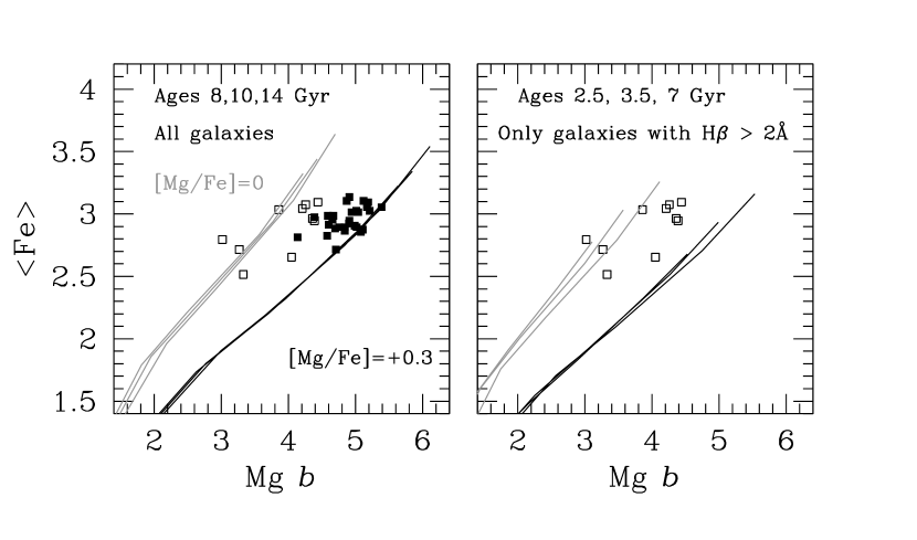
Figure 28.— Trager et al. data compared with our models in $<Fe>$–Mg $b$ diagrams. Left Panel: All galaxies are compared with solar-scaled (gray) and Mg-enhanced models. Galaxies with mean stellar ages younger than $\sim$ 7 Gyr ($H\beta>2{\rm\AA}$) are plotted with open symbols. Older galaxies (solid squares) tend to have higher [Mg/Fe] than their younger counterparts. Right panel: Same plot, comparing only galaxies with ages lower than $\sim$ 7 Gyr with models for younger single stellar populations with solar-scaled (gray) and Mg-enhanced abundance patterns. Galaxies with younger mean stellar ages in the Trager et al. sample tend to have lower [Mg/Fe].

6.2. Stellar Populations in the Blue

6.2.1 The Eisenstein et al. (2003) Sample

Finally, we get to the point of comparing our model predictions to galaxy data covering the full range of line indices considered in this paper. We are especially interested in contrasting the results based on blue and red indices. Until recently, high quality data for blue Lick indices were rare, if not entirely absent. The situation is changing quickly, as surveys of galaxies in the local and distant universe call for the need of a better understanding of the blue spectral region. A number of recent studies provided blue Lick index measurements based on moderate-to-high S/N spectra (e.g., Denicoló et al. 2005a,b, Rampazzo et al. 2005, Nelan et al. 2005, Sánchez-Blázquez et al. 2006a). We choose to analyze the stacked spectra from the Sloan Digital Sky Survey (SDSS) by Eisenstein et al. (2003). Our choice is chiefly motivated by the the fact that the stacked spectra are available publicly, so that we can perform our own index measurements and, most importantly, apply our own corrections for the effects of $\sigma$-broadening and Balmer line emission in-fill. Moreover, the stacked spectra have very high S/N ($>$ 400/${\rm\AA}$). Our procedure was described in Schiavon et al. (2006), but we briefly discuss the main aspects here.

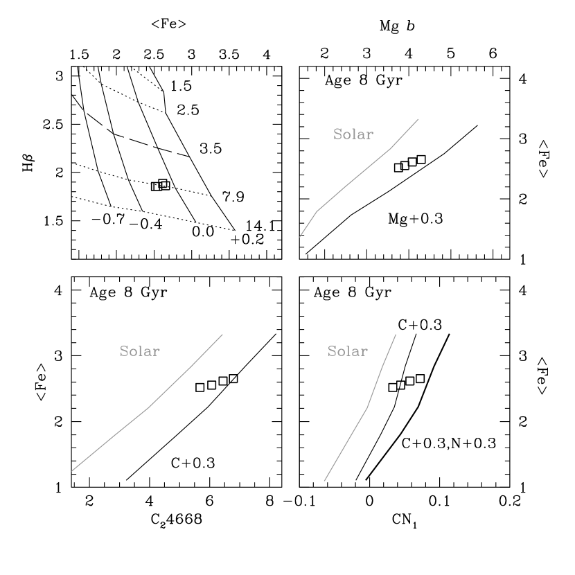
Figure 29.— Comparison of Lick indices measured in SDSS stacked spectra (“All” from Eisenstein et al. 2003) and our predictions for single stellar populations. Galaxy absolute luminosity increases from left to right (see $M_{r}$ values in Table 13). Errorbars are always smaller than symbol size. Upper left: The SDSS sample under study has a mean age of $\sim$ 8 Gyr (regardless of luminosity) and [Fe/H] just below solar (slightly dependent on luminosity) Upper right: In this and the remaining panels, galaxies are compared with solar-scaled (gray lines) and enhanced models (enhanced elements indicated in the labels). SDSS galaxies are Mg-enhanced, with more luminous galaxies being slightly more enhanced. Lower left: Galaxies are C-enhanced, with more luminous galaxies being more enhanced. Lower right: Three model predictions are shown: solar scaled (gray), C-enhanced (thin), and C,N-enhanced (thick). C-enhancement alone is not enough to match CN data, which require N-enhancement as well. More luminous galaxies are clearly more enhanced here.

The Eisenstein et al. (2003) sample consists of spectra of thousands of early-type galaxies from SDSS selected in terms of color (red) and morphology (bulge-dominated), with redshifts between $0.1<z<0.2$ (MAIN sample). The individual galaxy spectra sample a circular 3″ region centered on each galaxy and the spectral resolution is $\sim$ 170 km s^-1 (FWHM). Galaxies were assigned to bins according to luminosity and environment, and all individual spectra within each bin were coadded so as to generate very high S/N spectra as a function of luminosity and environmental density. The main properties of the Eisenstein et al. sample are summarized in their Table 1. We choose to analyze their “All” sample, which refers to galaxies binned only by luminosity, regardless of environmental density. Because each luminosity bin includes galaxies of all environments, the number of coadded spectra per bin is always in excess of 2,500, so that the S/N of each stacked spectrum is extremely high. Our sample therefore consists of 4 spectra, one for each of the 4 luminosity bins in Eisenstein et al. (2003) sample (Table 13 and Table 1 in Eisenstein et al. ). We note that $M_{r}^{\star}\approx-20.8$ for this sample (Blanton et al. 2001), so that our results refer to bright galaxies only. The spectra were downloaded from D. Eisenstein’s website (http://cmb.as.arizona.edu/^∼eisenste/).

6.2.2 Index Measurements

Figure 30.— Mean luminosity-weighted metal abundances and ages of the stellar populations in the SDSS galaxies from the Eisenstein et al. (2003) “All” sample, as a function of absolute magnitude in the SDSS $r$ band. Note that $M^{\star}_{r}\approx-20.8$ at the involved redshifts. All panels have a vertical scale of 0.5 dex. Iron abundances are slightly below solar for all luminosities, and abundance ratios are above solar for all elements in almost all luminosity bins. All abundances and all abundance ratios appear to be correlated with luminosity at different levels. Nitrogen is the most strongly enhanced element and also the one whose enhancement appears to be the most strongly correlated with galaxy luminosity. We find no correlation between mean age and luminosity (but see Figure 31).

Table 13Data for stacked SDSS spectra of early-type galaxies from Eisenstein et al. (2003)

$<M_{r}>$	[OII] $\lambda$3727	$H\delta_{A}$	$H\delta_{F}$	CN1	CN2	Ca4227	G4300	$H\gamma_{A}$	$H\gamma_{F}$	Fe4383	C24668	$H\beta$	Fe5015	Mg2	Mg $b$	Fe5270	Fe5335	$\sigma$ (km/s)
–20.78	1.73	–0.56	0.85	0.0332	0.0607	0.94	4.82	–4.58	–0.85	4.08	5.68	1.85	4.10	0.2288	3.76	2.63	2.41	190
–21.25	1.49	–0.79	0.76	0.0447	0.0725	0.94	4.89	–4.77	–0.95	4.20	6.07	1.85	4.32	0.2367	3.90	2.66	2.44	210
–21.73	0.82	–1.13	0.61	0.0575	0.0870	0.98	5.00	–5.10	–1.14	4.32	6.45	1.89	4.53	0.2464	4.08	2.72	2.51	240
–22.19	0.06	–1.45	0.47	0.0724	0.1046	1.04	5.17	–5.41	–1.33	4.57	6.79	1.86	4.85	0.2601	4.30	2.75	2.56	270
error	0.02	0.02	0.01	0.0005	0.0005	0.01	0.02	0.02	0.01	0.03	0.03	0.01	0.04	0.0002	0.01	0.02	0.02	20

Table 14Mean Ages (Gyr) and Metal Abundances from the Eisenstein et al. (2003) SDSS Stacked Spectra

$<M_{r}>$	Age($H\beta$)	Age($H\delta_{F}$)	[Fe/H]	[C/Fe]	[N/Fe]	[Mg/Fe]	[Ca/Fe]
–20.78	8.2	3.8	–0.17	0.08	0.12	0.19	0.02
–21.25	8.1	4.6	–0.15	0.12	0.17	0.21	0.06
–21.73	7.4	5.2	–0.10	0.13	0.28	0.22	0.10
–22.19	7.6	6.1	–0.08	0.15	0.38	0.26	0.17
error	0.3	0.2	0.01	0.03	0.04	0.02	0.05

All Lick indices of interest were measured in the stacked spectra using lick_ew, an idl routine written by G. Graves (for a description, see Graves & Schiavon 2006, in preparation). Before we can compare these measurements with our models, we need to correct the line indices for the effect of $\sigma$-broadening. That of course requires measuring first the velocity dispersions directly in the stacked spectra. We proceeded as follows. Velocity dispersions were measured through Fourier cross correlation using the IRAF rv.fxcor routine. The templates adopted were model single stellar population spectra calculated for a range of ages and metallicities, as described in Paper I. The choice of template is very important and can introduce important systematic effects if not carefully done. For each spectrum, a first guess of $\sigma$ is made, the indices are corrected and initial values of age and [Fe/H] are determined, if these values do not agree with those of the initial single stellar population template, a new template is adopted with the estimated age and [Fe/H] and the process is iterated until convergence is attained.

After velocity dispersions are determined, the indices can be corrected to their standard $\sigma=0$ values. These corrections were estimated again using model spectra of single stellar populations with appropriate ages and metallicities. Listings of such corrections for a set of representative ages and velocity dispersions are provided in Tables A14 through A17 in the Appendix.

The last step before we can compare models and data is the correction of Balmer line indices for the effect of emission line in-fill. Balmer line emission was estimated from the equivalent width of the [OII] $\lambda$ 3727 ${\rm\AA}$ line adopting a ratio between that line and $H\alpha$ given by EW[OII]/EW($H\alpha$) = 6. This value was taken from Yan et al. (2006), who studied the emission line properties of a large sample of SDSS galaxies. They found that most line-emitting red galaxies in SDSS tend to present LINER-like line ratios (see also, e.g., Phillips et al. 1986 and Rampazzo et al. 2005). Emission EWs for higher-order Balmer lines are obtained from EW($H\alpha$) by assuming standard values for the Balmer decrement (in the absence of reddening) and continuum fluxes measured in the stacked spectra. In this way, one obtains EW($H\beta$)/EW($H\alpha$)=0.36, EW($H\gamma$)/EW($H\alpha$)=0.19, and EW($H\delta$)/EW($H\alpha$)=0.13. Corrected indices and the velocity dispersions measured in the stacked spectra are listed in Table 13. The equivalent widths of the [OII] line, measured according to the definition of Fisher et al. (1998), are also provided in that Table

Before attempting quantitative estimates of mean ages and metal abundances of SDSS early-type galaxies, we compare the indices, measured as described above, with our model predictions in Figure 29. In all plots, error bars are smaller than symbol sizes and galaxy luminosity increases from left to right. In the upper left panel, data are compared with solar-scaled models in the $<Fe>$-$H\beta$ plane. Because these indices are essentially insensitive to abundance ratio effects, this plot allows us to obtain a first estimate of mean age and [Fe/H]. The result is that the stacked spectra indicate approximately the same mean age ($\sim$ 8 Gyr), regardless of luminosity. On the other hand, [Fe/H] is just below solar, and seems to be weakly correlated with luminosity.

In the remaining panels, SDSS early-type galaxies are compared with models in index-index planes that are sensitive to the abundances of magnesium, carbon, and nitrogen. In all these diagrams, solar-scaled (gray lines) models are plotted along with models computed with the abundances of a few key elements enhanced by +0.3 dex. In the upper right panel, the data are compared with solar-scaled and magnesium-enhanced models for an age of 8 Gyr, in the $<Fe>$-Mg $b$ plane. This plot suggests that early-type galaxies are enhanced in magnesium, with [Mg/Fe] slightly below +0.3. A slight correlation between Mg-enhancement and luminosity is apparent. In the lower left panel, data are compared with solar-scaled and carbon-enhanced models in the $<Fe>$-C₂4668 plane. Again in this case there is a clear indication of carbon-enhancement in early-type galaxies, with a more clear trend of carbon-enhancement as a function of luminosity than in the case of magnesium enhancement. Finally, in the lower right plot, data and models are compared in the $<Fe>$-CN₁ diagram. Because the CN₁ index is sensitive to both carbon and nitrogen enhancements, three models are displayed: solar scaled (gray) and carbon-enhanced (thin) models, plus models where both carbon and nitrogen are enhanced (thick). One can see that, while carbon-enhanced models do a good job of matching the C₂4668 index, the same is not true for CN₁ data, which are stronger than predicted by [C/Fe]=+0.3 models. In fact, matching CN₁ data requires that the abundance of nitrogen be also enhanced—thick lines do reach the high CN₁ values observed. One can also note that the correlation between enhancement and luminosity here is even stronger than in the case of the other plots.

Figure 31.— Mean ages of SDSS galaxies in the Eisenstein et al. (2003) sample, estimated from models including the abundance ratios from Figure 30 and Table 14. Upper panel: Ages according to $H\beta$ and $H\delta_{F}$. As expected from Figure 29, mean ages according to $H\beta$ are $\sim$ 8 Gyr, regardless of luminosity. On the other hand, ages according to $H\delta_{F}$ are substantially (2-4 Gyr) younger, with ages according to $H\gamma_{F}$ (not shown) lying somewhere inbetween. Lower panel: Differences between $H\delta_{F}$-based and $H\beta$-based ages, as a function of luminosity. The mismatch between $H\beta$ and $H\delta_{F}$-based ages is very luminosity dependent, being larger for lower luminosity galaxies.

Figure 32.— Data for the lowest luminosity bin ($<M_{r}>$ = –20.8) compared with single stellar population models in Balmer-metal line planes. Model ages are the same as upper left panel of Figure 29. To help guiding the eye, the 3.5 Gyr models are connected by dashed lines. The models were computed for the best-matching abundance pattern (Table 14), as can be seen by the good match to C₂4668 (see Section 6.2.4 and Figure 30). Therefore, abundance-ratio effects on $H\gamma_{F}$ and $H\delta_{F}$ are accounted for. The bluer the Balmer line, the younger the mean age that is estimated. The effect is independent of the metal index adopted.

With these qualitative results in mind, we apply our method described in Section 4.4 in order to obtain quantitative estimates of mean ages and metal abundances of the stellar populations of galaxies in the Eisenstein et al. (2003) sample, on the basis of the line indices measured in their spectra. The results are listed in Table 14 and shown in Figure 30, where resulting abundance ratios and mean ages are plotted as a function of mean $r$-band absolute magnitude. As expected from the discussion above, abundance ratios vary strongly as a function of mean luminosity. We will return to this issue in Section 6.2.4, but first discuss the mean ages of early-type galaxies in the next section.

6.2.3 Mean Ages and the History of Star Formation of Early-type Galaxies

We start by looking at the mean ages estimated from the different Balmer lines. According to Figures 29 and 30, early-type galaxies have luminosity-weighted mean ages of 8 Gyr, and no correlation is found between mean age and luminosity. The method described in Section 4.4 uses $H\beta$ as the only age indicator, due to its outstanding insensitivity to spectroscopic abundance ratio effects (Section 4.3.2). It is reasonable to expect, however, that other line indices should yield consistent ages when data are compared with models computed for the right abundance pattern. The latter is an important precaution, as the $H\delta$ and $H\gamma$ indices studied here are susceptible to spectroscopic abundance ratio effects, so that these indices can only be used for age estimates using models computed for the abundance pattern estimated above (Figure 30). In Figure 31, ages estimated from $H\beta$ and $H\delta_{F}$ are plotted against $<M_{r}>$. Ages according to $H\delta_{F}$ are consistently lower, with the difference ranging between 2 (25%) and 4 Gyr (50%). The differences are several times larger than the internal error bars (which are very small, thanks to the exceedingly high S/N of the stacked spectra).

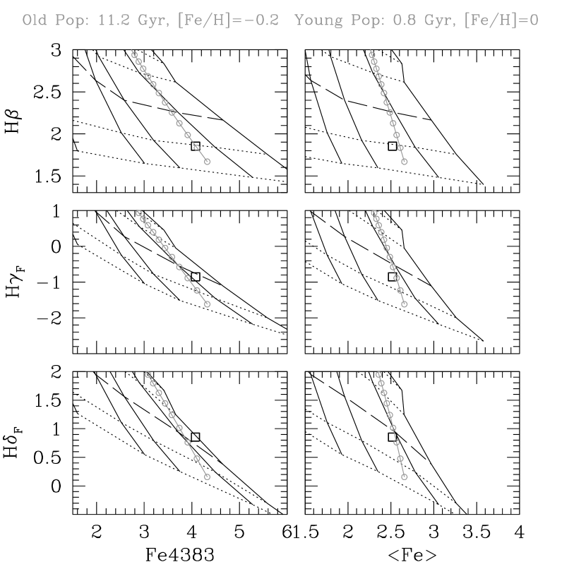
Figure 33.— Comparison between data for the lowest luminosity bin and a family of composite two-population models, consisting of an old single stellar population with an age of 11.2 Gyr and [Fe/H]=–0.2 combined with a young population with age 0.8 Gyr and solar metallicity. The contribution of the young population to the total mass budget is varied in steps of 0.5%, indicated by the gray open symbols. The largest the contribution of the young population to the mass budget, the stronger (weaker) the Balmer (metal) index for the composite population. A best match is obtained when the mass allocated in the young population is somewhere between $\sim$ 0.5 and 1% of the total mass. A similarly good match is obtained when the young component is $\sim$ 1 Gyr old, but in that case the mass fraction is an order of magnitude higher. See discussion in text.

It is interesting to verify how this effect manifests itself in index-index plots where Balmer and metal line indices are compared with models. Unfortunately, we cannot compare models and data for the different luminosity bins all in the same set of plots, as $H\delta$ and $H\gamma$ indices are strongly sensitive to abundance-ratio effects requiring different sets of single-stellar population models to be computed for each luminosity bin, so that plotting various sets of models in the same graph would make things look rather confusing. Therefore, we henceforth focus on the lowest luminosity bin, for which the age differences are the highest. In Figure 32, data for the $<M_{r}>=-20.8$ bin are compared to best-fitting models in $<Fe>$-Balmer and C₂4668 planes. From this figure, we learn that the age according to $H\delta_{F}$ is $\sim$ 4 Gyr (the data are just below the 3.5 Gyr dashed line), while that according to $H\beta$ is twice as old. The age according to $H\gamma_{F}$ lies somewhere in-between those values. In order for the $H\delta_{F}$-based age to agree with that based on $H\beta$, $H\delta_{F}$ would have to be $\sim$ 0.45 ${\rm\AA}$ weaker than the measured value which is entirely ruled out by the very small error bars of the measurements (Table 13). We note that the models are a very good match to the C₂4668 and CN (not shown) indices, so that in principle abundance-ratio effects on $H\delta_{F}$, which are mostly due to carbon and nitrogen abundances, are accounted for. While the focus of this discussion is on $H\delta_{F}$, we emphasize that this trend is quite general, in that bluer Balmer lines tend to indicate younger ages.

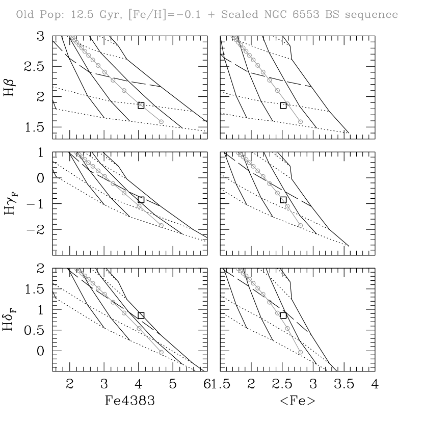
Figure 34.— Comparison between data for the lowest luminosity bin and a family of composite two-population models, consisting of an old single stellar population with an age of 11.2 Gyr and [Fe/H]=–0.2 combined with blue stragglers from the metal-rich Galactic globular cluster NGC 6553. The specific frequency of blue stragglers is varied in steps of 100 stars per 10⁴ $L_{\odot}$. Adding blue stragglers to an old population, one can match the data reasonably well, but only for extremely high blue-straggler specific frequencies. See details in text.

No such inconsistency was found when models were confronted with cluster data (Section 5), especially in the case of M 67, whose age and metallicity are comparable with those of SDSS early-type galaxies. Therefore, model inconsistencies cannot be blamed for the age differences apparent in Figures 30 through  32. We must seek other explanations. It is conceivable that the corrections for emission line in-fill are introducing a systematic effect in our Balmer line indices, since the relative corrections depend on assumptions on the size of the Balmer decrement and on the absence of reddening. However, it is very hard to attribute this discrepancy to errors in the Balmer in-fill corrections, for the following reason. The corrections for $H\beta$ and $H\delta_{F}$ were respectively $\sim$ 0.3 and 0.1 ${\rm\AA}$. Supposing we have overestimated the correction, the discrepancy between the two ages would be enhanced. In the extreme case, of no correction at all, the age according to $H\beta$ would be $\sim$ 14 Gyr and that according to $H\delta_{F}$ would be about 5 Gyr, which would increase the age discrepancy from a factor of two to a factor of three. Admitting that our in-fill corrections were instead underestimated, we can compute the size of the correction needed to bring the $H\beta$ and $H\delta_{F}$-based ages into agreement. The result is that the correction to $H\beta$ would have to be $\sim$ 0.7 ${\rm\AA}$, or more than twice the correction adopted. That is clearly ruled out by the small errors in the [OII] equivalent widths, and continuum measurements, as well as reasonable assumptions for the uncertainties in the Balmer decrement. Moreover, it would drive all the ages to much lower values, below 3.5 Gyr for ages according to $H\beta$, which would be in stark disagreement with all previous work on stellar age estimates in early-type galaxies. Therefore we conclude that systematic errors in our emission line in-fill corrections cannot account for the age discrepancies found.

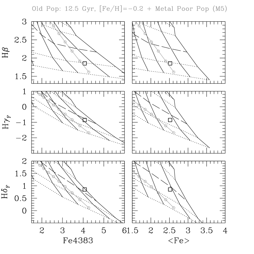
Figure 35.— Comparison between data for the lowest luminosity bin and a family of composite two-population models, consisting of an old single stellar population with an age of 11.2 Gyr and [Fe/H]=–0.2 combined with an old metal-poor population, represented by data from a Galactic globular cluster (M 5/NGC 5904). The contribution of the metal-poor population to the total mass budget is varied in steps of 5%, indicated by the gray open symbols. The match to the data is very poor, as these models cannot reproduce the strengths of all Balmer lines.

In the absence of systematic effects introduced by our in-fill corrections, another very likely possibility is that stellar populations that are unaccounted by the models may be affecting the line indices differentially. It is conceivable that the trend seen in Figure 32 may be caused by the contribution of warm stars (spectral types A to early-F), which are characterized by strong Balmer lines. The contribution by these stars to the integrated light peaks in the far blue, and falls steeply longward, so that they tend to affect more strongly higher order Balmer lines, located further into the blue. A similar effect was found by Schiavon et al. (2004b) in data for Galactic globular clusters. In that case, the warm star component was identified with blue HB stars, but young/intermediate-age stars are likely to have the same effect on the integrated light of galaxies. Abundance ratios that are not accounted for in our models could in principle also generate this type of systematic effect. In what follows we consider four possible explanations for this trend of mean ages with Balmer line: 1) Contamination of the integrated light by a small fraction, by mass, of a young/intermediate-age stellar population; 2) Contamination by blue stragglers; 3) Metal-poor stellar populations with a blue horizontal branch; and 4) Abundance-ratio effects. In what follows we examine briefly each one of these scenarios.

Young/Intermediate-age Stars: In order to test this possibility, we extended our model calculations to ages as low as 0.1 Gyr, for [Fe/H]=0 and +0.2. These computations should be taken with caution, because the fitting functions underlying our models did not take into account the effect of metallicity for stars hotter than $\sim$ 7500 K. The latter effect, however, is likely to be small, so we can adopt these calculations at least for a first examination of our working hypothesis. We generate families of two-component models, whose input parameters are the age and metallicity of the old component, the age of the young component and the fractional contribution of the latter to the total mass. The abundance pattern assumed for the old component is that listed in Table 14, and both the metallicity and abundance pattern of the young component are assumed to be solar. The input ages considered for the old component varied between 10 and 14 Gyr and [Fe/H] varied between –0.4 and 0. The age of the young component was varied between 0.1 and 1.2 Gyr. The fractional contribution of the young component to the total mass of the system was varied between 0 and 20%. A $\chi$-square minimization procedure was adopted to find the model that best matches the data for the Balmer and Fe indices. For simplicity, indices which are prime indicators of other abundances than iron were not included in the minimization, in order to avoid having to include the abundance ratios of the young component as another parameter in the two-component models. In Figure 33 the gray lines show the predictions of the family of two-component models, containing the best fitting model. The gray open circles indicate increments of the mass fraction allocated to the young component in steps of 0.5%. One can see that, as that fraction increases, Balmer lines get stronger and metal lines get weaker, due to the increasing contribution to the integrated light by hot stars. It is also apparent that the bluer indices are more strongly affected. For instance, when the young stars make up 2% of the total mass (fourth open circle from the bottom up) $H\delta_{F}$ indicates a single stellar population age lower than 3.5 Gyr, while the $H\beta$-based age would be $\sim$ 5 Gyr. The old component of the best fitting model has an age of 11.2 Gyr and [Fe/H]=–0.15, whereas the young component is 0.8 Gyr-old, contributing $\sim$ 0.5–1% of the total mass of the system. We note that this result is somewhat degenerate, as other families of models provide an equally good fit. If one increases the age of the young component, a good match can still be found to the data if its contribution to the total mass budget is increased by an adequate factor. This degeneracy is well known from studies of post-starbust galaxies and it can be broken by introducing age indicators further to the blue (Leonardi & Rose 1996). Most importantly, we note that the two-component model is a better match to the data than single stellar population models. It is also a better match to the data than the alternative models considered below. We note that a similar result was obtained by Sánchez-Blázquez et al. (2006a), who estimated younger ages from r.m.s. fitting of the blue part of their galaxy data. They interpreted their result as being due to a spread of stellar population ages in their sample galaxies. Interestingly, we find that the age discrepancy is larger for lower luminosity galaxies. If our interpretation is correct, this result tells us that star formation was more extended in lower mass galaxies, which is in agreement with findings by other authors (e.g., Caldwell et al. 2003, Bernardi et al. 2005, Gallazzi et al. 2006) and seems to lend support to the downsizing scenario (Cowie et al. 1996).

Blue Stragglers: Another family of warm stars which can potentially enhance Balmer lines in integrated spectra of galaxies are the blue stragglers. In paper III we showed that blue stragglers have a strong impact on the integrated spectrum of M 67, by markedly increasing the Balmer lines strengths in the cluster spectrum, which indicates substantially younger ages ($\sim$ 1.5 Gyr) than the known 3.5 Gyr age of the cluster. We also found that, as in the case of the galaxy spectra discussed here, the age of the cluster seems younger according to bluer Balmer lines. In order to test the blue straggler hypothesis, we perform the following test. We extracted colors and magnitudes of blue stragglers from the VI color-magnitude diagram of the metal-rich globular cluster NGC 6553 by Zoccali et al. (2001). Blue stragglers are known to be very abundant in this cluster (e.g., Beaulieu et al. 2001). We choose to use the Zoccali et al. data because these authors used observations at different epochs in order to measure the proper motion of the cluster, so that we can minimize foreground contamination of our blue straggler selection. Stars were considered as blue stragglers in NGC 6553 if they met the following criteria: $V>19.4$, $(V-I)<1.68$, and relative proper motion smaller than 0.1 arcsec (see Zoccali et al. for details). The resulting blue straggler sample consisted of 50 stars, whose colors and magnitudes were de-reddened and converted into absolute magnitudes adopting E(V–I) = 0.90 (Barbuy et al. 1998) and (m-M)₀=13.64 (Zoccali et al. 2001). The latter were used to compute effective temperatures and surface gravities using the Lejeune et al. (1998) calibrations and assuming [Fe/H]=–0.2 (Cohen et al. 1999, Barbuy et al. 2004) and 1$M_{\odot}$. The latter stellar parameters were used to generate line indices using the fitting functions presented in Section 3 for each blue-straggler star. The latter were integrated using the stars’ absolute magnitudes and colors in order to generate integrated indices of the blue straggler stars. The blue straggler indices were then used to generate a family of two-component models, by “contaminating” a reference old stellar population model with blue straggler light, assuming a range of blue straggler specific frequencies. The best match to the data was obtained when the old component was assumed to be 12.5 Gyr old, with [Fe/H]=–0.1. These models are compared with the observations in Figure 34, where the blue straggler specific frequency was varied from 0 to 1000 blue stragglers per 10⁴ $L_{\odot}$. The gray open symbols indicate steps of 100/10⁴ $L_{\odot}$. Figure 34 shows that adding blue stragglers to an old stellar population can also account for the trends observed in the data. However, the specific frequency needed to match the data is very high, ranging between 100 and 200 blue stragglers per 10⁴ $L_{\odot}$. As noted by Trager et al. (2000), typical specific frequencies found in Galactic globular clusters, whose characteristic core densities are much higher than those of early-type galaxies, range from a few to a few tens of stars per 10⁴$L_{\odot}$ (Ferraro, Fusi Pecci & Belazzini 1995). The case of M 67 is also definitely very extreme. In Paper III we saw that the spectrum of M 67 that includes blue stragglers has much stronger Balmer lines than the BS-free spectrum. But that spectrum includes star # 6481 (ID from Montgomery et al. 1993), with $T_{\rm eff}\mathrel{\hbox{\raise 2.15277pt\hbox{$>$}\hbox to0.0pt{\hss\lower 2.15277pt\hbox{$\sim$}}}}12,000K$ (Landsman et al. 1998) and several stars hotter than $\sim$ 8500 K. Such high temperatures are not expected to be found among lower mass blue stragglers characteristic of old, metal-rich, stellar populations. Moreover, M 67 has a specific blue straggler frequency that far exceeds that of other open clusters with the same central density (Landsman et al. 1998, Ahumada & Lapasset 1995), which is possibly the result of severe mass-segregation followed by evaporation of low mass stars (Hurley et al. 2001). In summary, while we cannot rule out the blue stragglers as the responsible for the apparent younger ages we are getting from higher-order Balmer lines, we deem this a less likely scenario, given the extreme conditions required to satisfy the data.

Old, Metal-Poor Populations: This scenario has been examined recently by Trager et al. (2005), so we will address it very briefly. It has been proposed by Maraston & Thomas (2000) that an old metal-poor stellar population component with a blue horizontal branch can account for the strong Balmer lines observed in integrated spectra of early-type galaxies. Moreover, their signature would be very similar to that found here, where higher order Balmer lines are more strongly affected (Schiavon et al. 2004b). In order to test this scenario, we adopt the line indices measured in the integrated spectrum of M 5, which were discussed in Section 5, and the integrated UBV colors of the cluster, taken from Van den Bergh (1967). The old, metal-poor, single stellar population thus produced is added to the old, metal-rich fiducial adopted in the previous exercises, to produce the two-component models shown in Figure 35. The open symbols indicate increments of 5% of the mass fraction of the metal-poor component, which is varied from 0 to 50%. While this model matches reasonably well the data for $H\beta$, it fails to satisfy the observations for $H\gamma_{F}$ and in particular those for $H\delta_{F}$. (see Trager et al. 2005 for a more detailed discussion). Varying the age of the prevalent old metal-rich population allows accommodating the data for one Balmer lines, at the expense of deteriorating the match to the others. We also tried using data for other globular clusters in the Schiavon et al. (2005) spectral library (NGC 2298 and 5986), but the quality of the match did not improve. The reason, we speculate, is that the temperature distribution of the warm stars in these old metal-poor stellar populations is not the one needed to match the data. We conclude that an old metal-poor component can not explain the behavior of Balmer lines in the data.

Abundance Ratios: Our models are a good match to the galaxy data for a number of spectral indices, which poses constraints on the abundances of iron, magnesium, carbon, nitrogen and calcium. Those are the elemental abundances that influence the most strongly the line indices studied in this paper. However, abundances of other elements such as oxygen, titanium, silicon, and sodium are largely unconstrained. Titanium, silicon, and sodium are spectroscopically active in the atmospheres of the stars that dominate the light in the systems under study, and the sensitivities of line indices as a function of these elements (Tripicco & Bell 1995, Korn et al. 2005) can be used as a guide to gauge the possible effects on the Balmer lines studied. These studies tell us that $H\beta$ is largely unaffected by abundance variations of elements other than iron, so we turn to $H\delta_{F}$. In order to bring the $H\delta_{F}$-based age into agreement with that based on $H\beta$, $H\delta_{F}$ would have to be decreased by roughly 0.45 ${\rm\AA}$. Of the three spectroscopically active elements, titanium is the one which affects $H\delta_{F}$ the most strongly. Inspection of the Korn et al. (2005) tables shows that a +0.3 dex variation in [Ti/Fe] causes $H\delta_{F}$ to drop by 0.31 ${\rm\AA}$ in the spectrum of a super-metal-rich giant star, 0.09 ${\rm\AA}$ for a turn-off star, and 0.22 ${\rm\AA}$ for a cool main sequence star. Therefore, in order to increase the model predictions to match $H\delta_{F}$ through a change in [Ti/Fe], the latter would have to be decreased by more than –0.7 dex (if we can trust linear extrapolations of the Korn et al. sensitivities). This sounds extreme. Similar reasoning poses even stronger lower limits on variations of silicon and sodium. Oxygen is more complicated, because it indirectly affects the line strengths via the dissociation equilibrium of CO and its impact on the strengths of more spectroscopically active carbon molecules, like CN and CH. This is accounted for in Korn et al.’s calculations, and consulting their tables we verify that only extreme variations of [O/Fe] can explain the $H\delta_{F}$ ages. However, oxygen can also play a role through its impact on stellar evolution. We saw in Section 4.3.1 that this effect is stronger on $H\beta$ than on $H\delta_{F}$ and found a slight, similar age trend on our comparisons with NGC 6528 data in Section 5.3, which we attribute to a slight mismatch between the oxygen abundances of the cluster and that of the isochrones. The trend is such that, in order to match $H\beta$ without affecting $H\delta_{F}$ substantially, [O/Fe] would have to be increased. Figure 12 shows how $H\beta$ changes when [O/Fe] varies from 0 to +0.5. Such a variation would account for about half of the effect seen in Figure 32, so that in order to account for the $H\delta_{F}$/$H\beta$ age mismatch [O/Fe] would probably need to be raised to $\sim$ +1.0 (again if linear extrapolations are to be trusted). While [O/Fe]=+1.0 may sound contriving, it cannot be ruled out. However, abundance determinations of stars in our closest proxy to the cores of early-type galaxies, the Galactic bulge field, seem to indicate much lower values for [O/Fe] (Fulbright et al. 2005). Therefore we conclude that, unless there is an important opacity source missing in the Korn et al. (2005) tables, and/or the effect of oxygen abundances on the evolutionary tracks of low-mass stars is quite substantially underestimated in the Padova isochrones, abundance ratio effects are a unlikely explanation for the differences we are finding between the ages determined from different Balmer lines.

In summary, while neither the blue straggler nor the abundance ratio scenarios can be completely ruled out, they seem to require extreme conditions in order to satisfy the observations. We conclude that contamination of the integrated light of the cores of galaxies by small mass fractions of young/intermediate-age stellar populations is the most likely scenario to account for the trends found. If this result is confirmed, the inference is that stellar population synthesis models are now able to constrain not only the mean ages of the stellar populations of galaxies from their integrated light, but also their distribution. This has been possible because the models adopted are extended to a wider baseline than previously considered and also because they match the data for known systems spanning the relevant range of stellar population parameters in an accurate and consistent fashion. This result also implies that the early-type galaxies studied have undergone a prolonged history of star formation, possibly with a small fraction of their stars being formed in the very recent past, as proposed in a number of previous works (e.g., O’Connell 1976, O’Connell 1980, Trager et al. 2000, to name a few). The ideal way of testing this scenario involves extending model and data accuracy towards an even wider baseline, preferably including the far blue and the ultraviolet.

6.2.4 Metal Abundances and the History of Chemical Enrichment of Early-type Galaxies

The abundance ratios obtained from application of our method described in Section 4.4 to estimate stellar population parameters from Lick indices are displayed in Figure 30. As expected from Figure 29, we find all galaxies to have iron abundances slightly below solar. There is a correlation between [Fe/H] and $M_{r}$, where [Fe/H] ranges between $\sim$ –0.15 for the faintest and just below solar for the brightest bin. Abundance ratios of all the elements studied relative to iron are solar or above solar, and are all correlated with luminosity to different degrees. That all elemental abundances are correlated with luminosity is an expected result, which derives from the more fundamental relation between mass and metallicity (e.g., Tinsley 1978). The interpretation of our results for abundance ratios is more subtle.

First and foremost, the most striking result in Figure 30 is the behavior of nitrogen abundances, both in absolute terms and as a function of luminosity. We caution that this result is sensitive to the abundance of carbon, which might be subject to systematics due to unknown oxygen abundances and/or theoretical uncertainties in the sensitivity of CN formation to carbon abundance variations (see Korn et al. 2005 for a discussion). Taking our results at face value, we find nitrogen to be enhanced in this SDSS sample, with [N/Fe] varying from just above solar, in the low luminosity end, to $\sim$ +0.2 for the highest luminosity bin. In the Galaxy, [N/Fe] is essentially solar for stars in a wide range of iron abundance (c.f. Figure 5). The only stellar systems known where [N/Fe] departs strongly from solar are globular clusters, where its mean value can be as high as $\sim$ +0.8. (e.g., Cannon et al. 1998, Cohen et al. 2002, Briley et al. 2004, Carretta et al. 2005, Lee 2005, Smith & Briley 2006). In fact, stars in globular clusters present a wide range of nitrogen abundances, and the distribution of this parameter seems to be bimodal. Globular clusters in M 31 seem to be even more nitrogen-rich than those in the Galaxy (Burstein et al. 1984, Li & Burstein 2003). However, the leading scenarios attempting to explain those nitrogen abundances tend to invoke conditions that are only met in globular clusters (e.g. Cannon et al. 1998, Beasley et al. 2004, Carretta et al. 2005).

Nitrogen is one of the elements whose history of enrichment is the most uncertain. The main source of nitrogen enrichment seems to be mass loss by intermediate and low mass AGB stars (e.g., Timmes et al. 1995, Henry & Worthey 1999, Chiappini, Romano & Matteucci 2003, Gavilán, Mollá & Buell 2006), but explosive nucleosynthesis in high-mass stars can also contribute nitrogen, especially at early times (e.g., Chiappini, Matteucci & Ballero 2005). The strong correlation of [N/Fe] with luminosity and (presumably) metallicity, seems to be indicating a strong secondary contribution to the enrichment of nitrogen in the sample studied (e.g., Tinsley 1979). If this interpretation is correct, nitrogen abundances may pose a novel constraint on the timescale for star formation in early-type galaxies. Secondary contribution to nitrogen enrichment is predominantly due to stellar winds from AGB stars with zero-age-main-sequence masses in the 4-8 $M_{\odot}$ range (Chiappini et al. 2003), whose lifetimes, according to the Geneva evolutionary tracks (Lejeune & Schaerer 2001), are of the order of 40-200 Myr. If the strong dependence of [N/Fe] on galaxy luminosity (and, presumably, mass) is a signature of secondary nitrogen enrichment, star formation in early-type galaxies must have lasted for at least 40-200 Myr in order for nitrogen contributed by these intermediate mass stars to be incorporated into new generations of stars. Therefore, our result for the run of nitrogen abundances as a function of galaxy luminosity may be setting a lower limit for the duration of star formation in early-type galaxies. This is a new constraint on the timescale of star formation in these systems. It is clearly possible to obtain tighter constraints on the basis of calculations from chemical evolution models, taking into consideration up-to-date stellar yields as a function of mass and a realistic IMF.

We find that all galaxies in the sample under study are magnesium-enhanced ([Mg/Fe]$>$0), and that more luminous galaxies are more enhanced than their fainter counterparts. As discussed in Section 6.1, this is a well known result, commonly interpreted as being due to the fact that the bulk of the stars in these galaxies were formed in a major event which lasted no longer than $\sim$ 1 Gyr, so that supernova type Ia could not contribute significantly to chemical enrichment (e.g., Wheeler et al. 1989). The correlation between [Mg/Fe] and luminosity has also been found by other authors (e.g., Trager et al. 2000, Denicoló et al. 2005, Thomas et al. 2005, Mendes de Oliveira et al. 2005) and is usually interpreted as being due to shorter star formation time-scales in more massive galaxies. This result is in sync with our finding that star formation in lower luminosity galaxies seems to have lasted longer than in their more luminous counterparts (Section 6.2.3), based on the $H\delta_{F}$-based ages. IMF variations as a function of galaxy mass could also account for these trends, but this hypothesis is more difficult to test.

As in previous studies (e.g., Vazdekis et al. 1997, Henry & Worthey 1999, Saglia et al. 2002, Thomas et al. 2003b, Prochaska et al. 2005) we find that calcium is not as enhanced relative to iron as magnesium. However, unlike most previous studies, we find that [Ca/Fe] seems to be well correlated with galaxy luminosity. As shown by Prochaska et al. (2005), and discussed in Section 4.3.2 the Ca4227 index is very strongly affected by CN. Once this effect is accounted for, either by redefining the index in order to minimize CN contamination (Prochaska et al. 2005) or by estimating the impact of CN lines on the index on the basis of spectrum synthesis calculations (this work), calcium is seen to be as correlated with galaxy luminosity as magnesium, which is the other $\alpha$-element in our analysis.

7. Conclusions

We presented a new set of models for the integrated absorption line indices and UBV magnitudes of single stellar populations. The models are based on the Jones (1999) spectral library, for which we determined a new set of homogeneous and accurate stellar parameters and a new set of fitting functions for Lick indices. Adopting theoretical isochrones from the Padova group, a set of reliable calibrations relating fundamental stellar parameters and colors, stellar abundances from the literature, which characterize the abundance pattern of the library stars, and sensitivity tables describing how line indices vary as a function of elemental abundance variations, we produced a new set of model predictions for Lick indices in single stellar populations. The models were extensively compared with superb data for Galactic clusters and nearby galaxies. Our main results can be summarized as follows:

1) Stellar parameters (effective temperature, surface gravity, and iron abundance) were determined for the 624 stars from the Jones (1999) library, based on semi-empirical calibrations of photometric and spectroscopic indices and fundamental stellar parameters. These parameters were contrasted with previous determinations from the literature and were found to be devoid of significant systematic effects. All stars for which substantial deviations from determinations by other groups were found were carefully examined and the best set of parameters was chosen. We show that accurate stellar parameters lie in the core of our ability to predict accurately the integrated indices of single stellar populations. The abundance pattern of the stellar library was characterized by surveying the literature for determinations of abundances of such key elements as iron, oxygen, carbon, nitrogen, magnesium, titanium, silicon, and calcium.

2) The above stellar parameters were combined with equivalent widths of line indices measured in the spectra of Jones library stars. This new equivalent width system is based on flux-calibrated spectra smoothed to the same resolution as that of the Lick/IDS system. Index measurements in the new system are substantially more accurate than those upon which the old Lick/IDS system is based. The two systems differ by small zero-point shifts. Polynomial fitting functions describing the behavior of 16 line indices as a function of effective temperature, surface gravity and iron abundance were computed. We compare our new fitting functions to those by Worthey et al. (1994) and found small but important improvements for some indices, which are mostly due to the best quality of the spectra and of the stellar parameters adopted.

3) The fitting functions are combined with theoretical isochrones from the Padova group in order to produce predictions of integrated line indices for single stellar populations. These are compared with high S/N data from four Galactic clusters spanning a representative range of ages, metallicities, and abundance patterns. We successfully match essentially all 16 line indices for the known input parameters (age, metallicity, abundance pattern, mass function) for each of the clusters considered. Our predictions for Fe indices, the Mg indices, C₂4668, the CN indices, and Ca4227 match the cluster data for [Fe/H], [Mg/H], [C/H], [N/H], and [Ca/H] within 0.1 dex of the known cluster values. Spectroscopic ages based on all Balmer line indices agree with those based on CMD analyses to within 1–2 Gyr for all clusters. We showed that the Ca4227 index is strongly influenced by CN lines. It is also shown that consistent results can only be obtained for Mg₂ and Mg $b$ if the appropriate (dwarf-depleted) mass function for the clusters is adopted, which means that a combination of these indices can potentially be used to set constraints on the IMF in the low mass regime.

4) Combining our single stellar population models with the abundance ratios for the library stars and the sensitivities of line indices to elemental abundances from Korn et al. (2005), we computed models for single stellar populations with several different abundance patterns. We devised a method that employs these models in order to estimate mean stellar ages and abundances of iron, magnesium, calcium, nitrogen and carbon. These models and method were tested against the observations of Galactic clusters with known abundance patterns with very satisfactory results. The models predict the cluster elemental abundances in agreement with the known values to within $\sim$ 0.1 dex. Spectroscopic ages agree with those based on analysis of cluster CMD data to within 1–2 Gyr, for all Balmer line indices considered. Using our model predictions for variable abundance ratios, we found that models with [Fe/H] = –0.1 $\pm$ 0.1 and a mild $\alpha$-enhancement, [$\alpha$/Fe] $\sim$ +0.1, are a better match to the data on NGC 6528 than those with higher enhancement. Matching the G band and CN indices, we found [C/Fe] $\sim$ -0.1 and [N/Fe] $\sim$ +0.5 as mean values for the stars in the core of NGC 6528. This mean abundance pattern resembles that of other well-known Galactic globular clusters such as 47 Tuc, M 71, and M 5, among others. This might suggest the carbon-nitrogen abundance dichotomy that characterizes these clusters is also present in NGC 6528.

5) The very good match obtained to data on Galactic clusters encouraged us to apply our models to observations of nearby galaxies. Initially, models were compared with the high quality measurements of $<Fe>$, Mg $b$, and $H\beta$ by Trager et al. (2000) for a sample of nearby galaxies. We reproduce their results, finding mean [Mg/Fe] $\sim$ +0.3, a spread in mean ages between 2.5 and 14 Gyr. We also found that [Fe/H] seems to decrease and [Mg/Fe] to increase when one goes from strong to low-$H\beta$ galaxies, in agreement with previous findings.

6) Our models were compared to high S/N measurements taken on stacked SDSS spectra of early-type galaxies from Eisenstein et al. (2003). Applying our method to determine mean ages and abundance ratios from Lick index measurements, we were able to estimate the abundances of iron, carbon, nitrogen, magnesium and calcium in these galaxies. We found that, while iron abundances are slightly below solar, the galaxies are enhanced relative to iron in all other elements. Iron abundances and all abundance ratios are shown to be positively correlated with luminosity. Unlike previous studies, we find that [Ca/Fe] is slightly enhanced in the sample studied. Among the elements studied, nitrogen is the one displaying the most conspicuous behavior, as it is the one whose enhancement is most strongly correlated with luminosity. This result might be subject to systematics due to uncertainties in the response of CN formation to carbon abundance variations, but we nevertheless speculate that it might be indicating the presence of a strong contribution by a secondary production mode. If this interpretation is correct, our result poses a constraint on the lower limit for the timescale for star formation in early-type galaxies (40–200 Myr). Magnesium is also seen to be enhanced and its enhancement is also correlated with luminosity, which is consistent with our finding that lower luminosity galaxies form stars for longer time periods (see below). More work is clearly needed to interpret these abundance ratio results.

7) Comparing the spectroscopic ages inferred from $H\beta$ and higher-order Balmer lines we found a systematic trend whereby the latter, especially $H\delta$, yield systematically younger ages than the former. Moreover, this discrepancy is stronger for lower luminosity galaxies. This is in strong contrast with the results from our analysis of cluster data, where we found that spectroscopic ages from all Balmer lines were remarkably consistent. We examined four possible scenarios to account for the observations: abundance-ratio effects, contamination by a small fraction of young/intermediate-age stars, by blue stragglers, and by metal-poor stellar populations with a blue horizontal branch. We argue that the metal-poor scenario cannot match the data and that the blue-straggler and abundance-ratio scenarios require extreme conditions to do so. Therefore, we conclude that the most likely explanation is a spread in the ages of the stellar populations in early-type galaxies. The implications are two-fold. On one hand, if this scenario is confirmed, stellar population synthesis will have evolved to a stage where it is now able to constrain not only the mean ages of stars in galaxies, but also their distribution. On the other, it implies that small amounts of star formation have occurred in the recent past in these nearby early-type galaxies. Our results suggest that on average lower luminosity galaxies formed stars until more recently than their more luminous counterparts, which lends further support to the “downsizing” scenario. Extending the accuracy of models and data blue-ward is the best way of further testing these results, posing stronger and more refined constraints on the history of star formation in early-type galaxies.

Appendix A Tables

Table 15The stellar library: fundamental parameters and line index measurements.

ID	$T_{\rm eff}$	$\log g$	[Fe/H]	$M_{\rm bol}$	$M_{\rm V}$	$(B-V)_{0}$	$H\delta_{F}$	$H\delta_{A}$	CN1	CN2	Ca4227
	G4300	$H\gamma_{F}$	$H\gamma_{A}$	Fe4383	C24668	$H\beta$	Fe5015	Mg $b$	Mg2	Fe5270	Fe5335
G12-24	5551	4.37	-0.11	4.82	4.87	0.67	-0.588	0.794	-0.052	-0.036	0.764
	5.340	-4.333	-0.615	3.139	3.139	2.500	3.547	3.333	0.130	2.058	1.698
G82-12	5610	3.93	-0.32	3.68	3.70	0.65	0.442	1.224	-0.071	-0.055	0.740
	5.066	-3.539	-0.177	2.634	2.934	2.508	3.249	2.522	0.125	1.846	1.539
G43-33	5774	3.98	-0.50	3.69	3.62	0.54	2.025	1.852	-0.082	-0.063	0.404
	4.088	-1.088	1.124	1.347	1.498	3.019	2.352	1.434	0.075	1.195	0.909
G44-6	5434	4.27	-0.46	4.79	4.90	0.60	0.633	1.275	-0.076	-0.061	0.635
	4.912	-3.210	-0.273	2.022	2.402	2.362	2.425	2.762	0.119	1.415	1.103
G74-5	5463	4.29	-0.91	4.92	4.99	0.57	1.155	1.494	-0.075	-0.059	0.520
	4.280	-2.231	0.229	1.553	0.783	2.303	1.674	2.313	0.092	1.135	0.856

Table 16Lick indices for single stellar populations: the base models computed with solar-scaled isochrones.

Age	[Fe/H]	$H\delta_{A}$	$H\delta_{F}$	CN1	CN2	Ca4227	G4300	$H\gamma_{A}$	$H\gamma_{F}$	Fe4383	C24668	$H\beta$	Fe5015	Mg $b$	Mg2	Fe5270	Fe5335
0.10	0.0	6.9379	5.8308	-0.1619	-0.1213	-0.0086	-1.1189	6.8475	5.8282	0.1518	0.6257	5.6665	1.4216	0.6712	0.0559	0.8318	0.7518
0.10	0.2	7.9228	6.4156	-0.1788	-0.1360	0.0330	-1.7570	7.9978	6.4615	-0.1183	0.4930	6.3683	1.2715	0.7950	0.0534	0.8059	0.7555
0.11	0.0	7.3434	6.0405	-0.1689	-0.1272	0.0049	-1.3225	7.1792	6.0209	0.0856	0.6180	5.9275	1.4137	0.7218	0.0548	0.8486	0.7458
0.11	0.2	8.3321	6.6142	-0.1873	-0.1437	0.0380	-1.9326	8.3291	6.6514	-0.1928	0.4743	6.5600	1.2435	0.7854	0.0516	0.7924	0.7217
0.13	0.0	7.8073	6.2780	-0.1760	-0.1329	0.0394	-1.5656	7.6137	6.2436	-0.0435	0.6610	6.2368	1.4856	0.8159	0.0505	0.8423	0.7302

Table 17Lick indices for single stellar populations: the base models computed with $\alpha$-enhanced isochrones.

Age	[Fe/H]	$H\delta_{A}$	$H\delta_{F}$	CN1	CN2	Ca4227	G4300	$H\gamma_{A}$	$H\gamma_{F}$	Fe4383	C24668	$H\beta$	Fe5015	Mg $b$	Mg2	Fe5270	Fe5335
0.10	0.0	8.1686	6.4731	-0.1824	-0.1385	0.0612	-1.7169	7.8668	6.3867	-0.0488	0.7528	6.3299	1.5202	0.9085	0.0582	0.9395	0.8202
0.10	0.3	8.9895	6.8871	-0.1970	-0.1517	0.1137	-2.0943	8.5524	6.7879	-0.0745	1.0056	6.6498	1.8321	1.0910	0.0707	1.1891	1.0672
0.11	0.0	8.5311	6.6415	-0.1899	-0.1453	0.0681	-1.8564	8.1572	6.5464	-0.1168	0.7293	6.4850	1.4952	0.9100	0.0572	0.9374	0.8045
0.11	0.3	9.3018	7.0218	-0.2029	-0.1570	0.1237	-2.1802	8.7989	6.9133	-0.1290	1.0121	6.7670	1.8428	1.0977	0.0700	1.1991	1.0660
0.13	0.0	8.8966	6.8068	-0.1974	-0.1521	0.0774	-1.9834	8.4562	6.7060	-0.1872	0.7037	6.6352	1.4751	0.9131	0.0564	0.9353	0.7914

Table 18Magnitudes computed using the solar-scaled isochrones.

Age	[Fe/H]	$M_{V}^{1}$	$(B-V)^{1}$	$(U-V)^{1}$	$M_{V}^{2}$	$(B-V)^{2}$	$(U-V)^{2}$
0.10	0.00	2.751	0.105	-0.375	2.661	0.121	-0.307
0.10	0.22	2.792	0.067	-0.247	2.763	0.088	-0.296
0.11	0.00	2.809	0.110	-0.321	2.736	0.126	-0.278
0.11	0.22	2.835	0.098	-0.247	2.834	0.091	-0.264
0.13	0.00	2.877	0.115	-0.272	2.805	0.137	-0.248
0.13	0.22	2.941	0.093	-0.213	2.896	0.102	-0.227

Table 19Magnitudes computed using the $\alpha$-enhanced isochrones.

Age	[Fe/H]	$M_{V}^{1}$	$(B-V)^{1}$	$(U-V)^{1}$	$M_{V}^{2}$	$(B-V)^{2}$	$(U-V)^{2}$
0.10	0.01	2.999	0.138	-0.187	2.924	0.150	-0.224
0.10	0.33	3.042	0.180	-0.146	2.992	0.173	-0.150
0.11	0.01	3.066	0.145	-0.184	2.995	0.154	-0.191
0.11	0.33	3.112	0.187	-0.110	3.063	0.181	-0.113
0.13	0.01	3.135	0.151	-0.149	3.070	0.158	-0.157
0.13	0.33	3.183	0.196	-0.074	3.136	0.189	-0.076

Table 20Lick indices computed for the abundance pattern of M 67 (Table 5).

Age	[Fe/H]	$H\delta_{A}$	$H\delta_{F}$	CN1	CN2	Ca4227	G4300	$H\gamma_{A}$	$H\gamma_{F}$	Fe4383	C24668	$H\beta$	Fe5015	Mg $b$	Mg2	Fe5270	Fe5335
1.20	-1.3	6.0966	4.5507	-0.1510	-0.1167	0.1300	0.8990	4.2798	3.9359	0.4553	0.6471	4.3633	1.5833	0.6659	0.0613	0.9834	0.8992
1.20	-0.7	5.9204	4.4215	-0.1427	-0.1078	0.1403	1.2615	3.9890	3.9140	0.7978	1.5563	4.6787	2.3875	1.0419	0.0647	1.3361	1.0691
1.20	-0.4	4.5117	3.6227	-0.0982	-0.0676	0.2991	1.9786	2.0874	2.9905	1.3462	2.2351	3.9965	3.1119	1.5158	0.0879	1.7320	1.4159
1.20	0.0	3.0096	2.8627	-0.0612	-0.0296	0.6182	2.3479	0.3124	2.1006	2.0694	2.8798	3.5384	4.0534	2.0061	0.1050	2.1810	1.8123
1.20	0.2	1.8031	2.2922	-0.0469	-0.0175	0.7568	2.8072	-0.8854	1.4197	2.7212	3.6400	3.3265	4.8045	2.3176	0.1170	2.5374	2.1519

Table 21 Lick indices computed for the abundance pattern of CN-strong stars in 47 Tuc, adopting the solar-scaled Padova isochrones by Girardi et al. (2000), and a dwarf-poor IMF ($x=-4$).

Age	[Fe/H]	$H\delta_{A}$	$H\delta_{F}$	CN1	CN2	Ca4227	G4300	$H\gamma_{A}$	$H\gamma_{F}$	Fe4383	C24668	$H\beta$	Fe5015	Mg $b$	Mg2	Fe5270	Fe5335
1.20	-1.3	4.0428	3.2702	-0.0698	-0.0372	0.1607	1.6833	1.7633	2.5923	0.8294	-0.7163	3.1227	2.5457	1.2904	0.0877	1.4054	1.1899
1.20	-0.7	4.5019	3.1747	-0.0260	0.0089	0.1922	1.7658	1.5785	2.6268	1.1471	0.4849	3.5153	3.6216	2.4293	0.1171	1.7448	1.3788
1.20	-0.4	3.3331	2.4454	0.0463	0.0790	0.4001	2.2906	-0.2106	1.7504	1.7669	1.1358	3.0013	4.3459	3.2696	0.1546	2.1175	1.7232
1.20	0.0	2.3064	1.9848	0.1121	0.1565	0.7977	2.1264	-1.3286	1.2597	2.5900	1.9413	2.7866	5.1696	4.1125	0.1899	2.6231	2.1925
1.20	0.2	1.3420	1.5803	0.1470	0.1896	0.9784	2.2197	-2.0882	0.8663	3.2612	2.7738	2.7021	5.8576	4.5784	0.2115	2.9997	2.5611

Table 22 Lick indices computed for the abundance pattern of CN-weak stars in 47 Tuc, adopting the solar-scaled Padova isochrones by Girardi et al. (2000), and a dwarf-poor IMF ($x=-4$).

Age	[Fe/H]	$H\delta_{A}$	$H\delta_{F}$	CN1	CN2	Ca4227	G4300	$H\gamma_{A}$	$H\gamma_{F}$	Fe4383	C24668	$H\beta$	Fe5015	Mg $b$	Mg2	Fe5270	Fe5335
1.20	-1.3 -4.00	4.0421	3.2061	-0.0893	-0.0571	0.3187	2.1494	1.4408	2.4116	0.9833	1.1672	3.1022	2.4769	1.2449	0.0999	1.4003	1.1890
1.20	-0.7 -4.00	4.1488	3.1160	-0.0944	-0.0646	0.4962	2.2658	1.2158	2.4324	1.3044	2.2431	3.4959	3.5577	2.3856	0.1286	1.7403	1.3775
1.20	-0.4 -4.00	2.8222	2.3877	-0.0483	-0.0229	0.7826	2.7939	-0.5636	1.5598	1.9242	2.9232	2.9816	4.2806	3.2263	0.1659	2.1128	1.7219
1.20	0.0 -4.00	1.7065	1.9373	-0.0086	0.0260	1.2329	2.6752	-1.7236	1.0545	2.7519	3.5962	2.7680	5.1090	4.0713	0.2006	2.6189	2.1907
1.20	0.2 -4.00	0.7096	1.5373	0.0127	0.0436	1.4399	2.7860	-2.4991	0.6556	3.4245	4.3793	2.6839	5.7985	4.5380	0.2219	2.9956	2.5591

Table 23Lick indices computed for the (CN-strong) abundance pattern of NGC 6528, adopting the solar-scaled Padova isochrones by Girardi et al. (2000) and a Salpeter IMF.

Age	[Fe/H]	$H\delta_{A}$	$H\delta_{F}$	CN1	CN2	Ca4227	G4300	$H\gamma_{A}$	$H\gamma_{F}$	Fe4383	C24668	$H\beta$	Fe5015	Mg $b$	Mg2	Fe5270	Fe5335
1.20	-1.3	6.2125	4.6109	-0.1263	-0.0879	-0.0422	0.7027	4.5141	4.0340	0.3101	0.5845	4.3444	1.4873	0.7496	0.0634	0.9345	0.8754
1.20	-0.7	6.3753	4.5593	-0.1031	-0.0621	-0.1291	0.9388	4.4001	4.0775	0.6039	1.3198	4.6511	2.2329	1.1794	0.0680	1.2514	1.0113
1.20	-0.4	5.1351	3.8033	-0.0488	-0.0108	-0.0327	1.5774	2.6077	3.1942	1.1094	1.8991	3.9629	2.9192	1.6805	0.0916	1.6247	1.3373
1.20	0.0	3.6539	3.0563	-0.0061	0.0331	0.2698	1.8513	0.9273	2.3510	1.8210	2.4877	3.4998	3.8611	2.2017	0.1097	2.0674	1.7295
1.20	0.2	2.5017	2.5061	0.0132	0.0507	0.3812	2.2481	-0.1853	1.7031	2.4469	3.2099	3.2841	4.5913	2.5298	0.1220	2.4105	2.0574

Table 24Model that best matches indices in the stacked SDSS spectrum for $<M_{r}>=-20.78$.

Age	[Fe/H]	$H\delta_{A}$	$H\delta_{F}$	CN1	CN2	Ca4227	G4300	$H\gamma_{A}$	$H\gamma_{F}$	Fe4383	C24668	$H\beta$	Fe5015	Mg $b$	Mg2	Fe5270	Fe5335
1.20	-1.3	6.0624	4.5588	-0.1415	-0.1069	0.0754	0.9920	4.2726	3.9342	0.4451	0.8816	4.3535	1.5240	0.9808	0.0775	0.9854	0.8854
1.20	-0.7	5.9609	4.4427	-0.1194	-0.0835	0.0352	1.4565	3.9224	3.8695	0.7880	2.3418	4.6637	2.2493	1.4704	0.0916	1.3197	1.0346
1.20	-0.4	4.5990	3.6567	-0.0672	-0.0353	0.1684	2.2135	2.0183	2.9363	1.3131	3.3004	3.9759	2.9203	2.0386	0.1220	1.7033	1.3671
1.20	0.0	3.1165	2.9026	-0.0284	0.0048	0.4895	2.6023	0.2010	2.0263	2.0477	4.1422	3.5140	3.8443	2.6546	0.1452	2.1507	1.7608
1.20	0.2	1.9267	2.3403	-0.0111	0.0201	0.6218	3.0820	-0.9986	1.3393	2.6822	5.0101	3.2985	4.5711	3.0414	0.1615	2.5004	2.0916

Table 25Model that best matches indices in the stacked SDSS spectrum for $<M_{r}>=-21.25$.

Age	[Fe/H]	$H\delta_{A}$	$H\delta_{F}$	CN1	CN2	Ca4227	G4300	$H\gamma_{A}$	$H\gamma_{F}$	Fe4383	C24668	$H\beta$	Fe5015	Mg $b$	Mg2	Fe5270	Fe5335
1.20	-1.3	6.0144	4.5497	-0.1376	-0.1029	0.0555	1.0543	4.2310	3.9145	0.4758	0.9799	4.3532	1.5203	0.9923	0.0792	0.9951	0.8851
1.20	-0.7	5.9490	4.4404	-0.1111	-0.0748	0.0188	1.5535	3.8486	3.8336	0.8088	2.6239	4.6610	2.2299	1.5033	0.0961	1.3279	1.0304
1.20	-0.4	4.5994	3.6570	-0.0564	-0.0239	0.1518	2.3294	1.9304	2.8929	1.3299	3.6811	3.9719	2.8918	2.0813	0.1279	1.7107	1.3605
1.20	0.0	3.1213	2.9041	-0.0171	0.0168	0.4739	2.7376	0.0842	1.9689	2.0720	4.5838	3.5092	3.8130	2.7098	0.1522	2.1583	1.7540
1.20	0.2	1.9318	2.3425	0.0013	0.0333	0.6068	3.2311	-1.1282	1.2750	2.7054	5.4880	3.2930	4.5365	3.1032	0.1692	2.5078	2.0833

Table 26Model that best matches indices in the stacked SDSS spectrum for $<M_{r}>=-21.73$.

Age	[Fe/H]	$H\delta_{A}$	$H\delta_{F}$	CN1	CN2	Ca4227	G4300	$H\gamma_{A}$	$H\gamma_{F}$	Fe4383	C24668	$H\beta$	Fe5015	Mg $b$	Mg2	Fe5270	Fe5335
1.20	-1.3	5.9878	4.5453	-0.1322	-0.0971	0.0352	1.0749	4.2175	3.9084	0.4772	1.0092	4.3527	1.5206	0.9990	0.0798	1.0050	0.8853
1.20	-0.7	5.9632	4.4432	-0.1015	-0.0646	0.0079	1.5825	3.8307	3.8246	0.8006	2.6977	4.6594	2.2251	1.5230	0.0976	1.3378	1.0282
1.20	-0.4	4.6299	3.6629	-0.0442	-0.0109	0.1437	2.3632	1.9111	2.8825	1.3160	3.7787	3.9696	2.8840	2.1069	0.1299	1.7207	1.3569
1.20	0.0	3.1547	2.9112	-0.0037	0.0310	0.4651	2.7741	0.0596	1.9560	2.0592	4.6963	3.5066	3.8051	2.7428	0.1546	2.1687	1.7505
1.20	0.2	1.9670	2.3508	0.0157	0.0487	0.5993	3.2710	-1.1545	1.2609	2.6893	5.6094	3.2901	4.5275	3.1397	0.1718	2.5184	2.0790

Table 27Model that best matches indices in the stacked SDSS spectrum for $<M_{r}>=-22.19$.

Age	[Fe/H]	$H\delta_{A}$	$H\delta_{F}$	CN1	CN2	Ca4227	G4300	$H\gamma_{A}$	$H\gamma_{F}$	Fe4383	C24668	$H\beta$	Fe5015	Mg $b$	Mg2	Fe5270	Fe5335
1.20	-1.3	5.9570	4.5428	-0.1271	-0.0918	0.0285	1.1130	4.1964	3.8988	0.4798	1.0721	4.3520	1.5181	1.0296	0.0815	1.0217	0.8848
1.20	-0.7	5.9926	4.4585	-0.0924	-0.0551	0.0309	1.6296	3.8164	3.8148	0.7752	2.8472	4.6552	2.2018	1.6140	0.1028	1.3513	1.0202
1.20	-0.4	4.6851	3.6868	-0.0327	0.0010	0.1802	2.4160	1.9022	2.8729	1.2741	3.9741	3.9635	2.8485	2.2269	0.1368	1.7324	1.3444
1.20	0.0	3.2149	2.9379	0.0086	0.0439	0.5040	2.8265	0.0471	1.9449	2.0175	4.9247	3.4996	3.7676	2.8937	0.1629	2.1806	1.7377
1.20	0.2	2.0336	2.3811	0.0290	0.0627	0.6430	3.3268	-1.1647	1.2495	2.6386	5.8562	3.2820	4.4852	3.3072	0.1809	2.5297	2.0636

Table 28Corrections to $\sigma=0$ km s^-1, for a 1.5 Gyr-old stellar population with solar metallicity.

$\sigma$ (km s-1)	$H\delta_{A}$	$H\delta_{F}$	CN1	CN2	Ca4227	G4300	$H\gamma_{A}$	$H\gamma_{F}$	Fe4383	C24668	$H\beta$	Fe5015	Mg $b$	Mg2	Fe5270	Fe5335
25	0.9993	1.0007	0.0000	0.0002	1.0028	1.0006	0.9998	1.0005	1.0015	1.0005	1.0004	1.0018	0.0000	1.0012	1.0018	1.0033
50	0.9973	1.0029	0.0001	0.0005	1.0112	1.0023	0.9992	1.0023	1.0062	1.0020	1.0016	1.0072	0.0001	1.0048	1.0071	1.0132
75	0.9939	1.0065	0.0003	0.0010	1.0253	1.0050	0.9983	1.0054	1.0139	1.0046	1.0036	1.0160	0.0002	1.0110	1.0159	1.0298
100	0.9893	1.0117	0.0005	0.0018	1.0453	1.0089	0.9974	1.0101	1.0246	1.0083	1.0064	1.0280	0.0004	1.0200	1.0280	1.0531
125	0.9839	1.0184	0.0008	0.0027	1.0713	1.0138	0.9968	1.0166	1.0384	1.0132	1.0100	1.0428	0.0005	1.0319	1.0431	1.0832
150	0.9776	1.0268	0.0011	0.0038	1.1035	1.0198	0.9968	1.0253	1.0551	1.0194	1.0143	1.0600	0.0007	1.0471	1.0610	1.1200
175	0.9708	1.0370	0.0015	0.0050	1.1425	1.0268	0.9977	1.0367	1.0748	1.0268	1.0195	1.0793	0.0009	1.0655	1.0813	1.1636
200	0.9636	1.0490	0.0019	0.0063	1.1885	1.0348	0.9998	1.0511	1.0974	1.0356	1.0257	1.1004	0.0012	1.0870	1.1036	1.2140
225	0.9563	1.0630	0.0023	0.0077	1.2422	1.0439	1.0035	1.0691	1.1230	1.0457	1.0329	1.1231	0.0014	1.1116	1.1278	1.2711
250	0.9491	1.0790	0.0027	0.0092	1.3040	1.0541	1.0090	1.0911	1.1515	1.0571	1.0415	1.1471	0.0017	1.1389	1.1535	1.3350
275	0.9421	1.0971	0.0031	0.0106	1.3747	1.0653	1.0164	1.1175	1.1831	1.0700	1.0514	1.1724	0.0019	1.1686	1.1807	1.4053
300	0.9355	1.1174	0.0035	0.0121	1.4555	1.0777	1.0261	1.1486	1.2178	1.0842	1.0630	1.1987	0.0023	1.2007	1.2092	1.4821
325	0.9293	1.1400	0.0039	0.0136	1.5470	1.0913	1.0380	1.1850	1.2559	1.0998	1.0762	1.2261	0.0026	1.2348	1.2391	1.5651
350	0.9239	1.1649	0.0043	0.0150	1.6508	1.1062	1.0525	1.2271	1.2973	1.1167	1.0913	1.2545	0.0030	1.2708	1.2705	1.6540
375	0.9191	1.1920	0.0046	0.0164	1.7678	1.1226	1.0695	1.2754	1.3424	1.1349	1.1084	1.2837	0.0034	1.3087	1.3035	1.7491
400	0.9151	1.2216	0.0050	0.0177	1.8997	1.1404	1.0892	1.3303	1.3915	1.1543	1.1276	1.3138	0.0039	1.3485	1.3386	1.8500

Table 29Corrections to $\sigma=0$ km s^-1, for a 3.5 Gyr-old stellar population with solar metallicity.

$\sigma$ (km s-1)	$H\delta_{A}$	$H\delta_{F}$	CN1	CN2	Ca4227	G4300	$H\gamma_{A}$	$H\gamma_{F}$	Fe4383	C24668	$H\beta$	Fe5015	Mg $b$	Mg2	Fe5270	Fe5335
25	1.0031	1.0011	0.0000	0.0001	1.0028	1.0003	0.9999	1.0004	1.0014	1.0006	1.0004	1.0018	0.0001	1.0011	1.0018	1.0032
50	1.0117	1.0047	0.0001	0.0004	1.0110	1.0014	0.9997	1.0017	1.0054	1.0022	1.0015	1.0072	0.0002	1.0045	1.0072	1.0129
75	1.0266	1.0106	0.0004	0.0010	1.0246	1.0032	0.9994	1.0036	1.0121	1.0050	1.0032	1.0161	0.0003	1.0104	1.0161	1.0290
100	1.0474	1.0190	0.0006	0.0018	1.0441	1.0057	0.9992	1.0051	1.0214	1.0090	1.0057	1.0281	0.0005	1.0190	1.0282	1.0517
125	1.0746	1.0303	0.0010	0.0028	1.0693	1.0089	0.9991	1.0058	1.0333	1.0142	1.0087	1.0428	0.0007	1.0303	1.0435	1.0809
150	1.1082	1.0446	0.0014	0.0039	1.1008	1.0128	0.9994	1.0043	1.0478	1.0208	1.0124	1.0600	0.0009	1.0447	1.0615	1.1168
175	1.1488	1.0622	0.0018	0.0052	1.1387	1.0175	1.0002	1.0000	1.0647	1.0286	1.0167	1.0792	0.0011	1.0621	1.0820	1.1595
200	1.1965	1.0832	0.0023	0.0066	1.1834	1.0229	1.0017	0.9920	1.0840	1.0379	1.0219	1.1001	0.0014	1.0824	1.1046	1.2087
225	1.2520	1.1084	0.0028	0.0081	1.2356	1.0292	1.0040	0.9795	1.1056	1.0485	1.0279	1.1225	0.0017	1.1056	1.1291	1.2648
250	1.3157	1.1379	0.0034	0.0097	1.2958	1.0362	1.0072	0.9630	1.1296	1.0605	1.0350	1.1461	0.0020	1.1314	1.1550	1.3274
275	1.3884	1.1722	0.0039	0.0113	1.3647	1.0441	1.0115	0.9425	1.1559	1.0739	1.0434	1.1709	0.0023	1.1595	1.1825	1.3966
300	1.4706	1.2116	0.0045	0.0129	1.4431	1.0530	1.0168	0.9185	1.1844	1.0887	1.0533	1.1966	0.0027	1.1899	1.2114	1.4722
325	1.5632	1.2569	0.0051	0.0145	1.5322	1.0630	1.0234	0.8918	1.2153	1.1048	1.0648	1.2233	0.0031	1.2224	1.2417	1.5541
350	1.6674	1.3085	0.0056	0.0161	1.6327	1.0740	1.0312	0.8637	1.2485	1.1223	1.0780	1.2508	0.0036	1.2568	1.2735	1.6421
375	1.7838	1.3668	0.0061	0.0177	1.7462	1.0863	1.0403	0.8348	1.2841	1.1411	1.0931	1.2791	0.0041	1.2931	1.3070	1.7362
400	1.9137	1.4330	0.0067	0.0192	1.8742	1.0999	1.0507	0.8059	1.3220	1.1611	1.1102	1.3081	0.0047	1.3315	1.3425	1.8362

Table 30Corrections to $\sigma=0$ km s^-1, for a 7.9 Gyr-old stellar population with solar metallicity.

$\sigma$ (km s-1)	$H\delta_{A}$	$H\delta_{F}$	CN1	CN2	Ca4227	G4300	$H\gamma_{A}$	$H\gamma_{F}$	Fe4383	C24668	$H\beta$	Fe5015	Mg $b$	Mg2	Fe5270	Fe5335
25	1.0012	1.0034	0.0001	0.0001	1.0027	1.0003	0.9999	1.0005	1.0013	1.0006	1.0004	1.0019	0.0001	1.0011	1.0018	1.0032
50	1.0047	1.0131	0.0002	0.0005	1.0106	1.0011	0.9997	1.0021	1.0051	1.0022	1.0014	1.0075	0.0002	1.0045	1.0071	1.0127
75	1.0104	1.0302	0.0004	0.0011	1.0239	1.0025	0.9994	1.0047	1.0114	1.0051	1.0029	1.0165	0.0003	1.0104	1.0158	1.0285
100	1.0184	1.0552	0.0007	0.0019	1.0427	1.0044	0.9992	1.0079	1.0202	1.0091	1.0051	1.0288	0.0005	1.0189	1.0279	1.0509
125	1.0286	1.0898	0.0011	0.0029	1.0670	1.0070	0.9991	1.0114	1.0314	1.0145	1.0078	1.0440	0.0007	1.0302	1.0428	1.0797
150	1.0408	1.1359	0.0015	0.0040	1.0975	1.0101	0.9993	1.0149	1.0450	1.0211	1.0109	1.0617	0.0010	1.0444	1.0606	1.1152
175	1.0550	1.1967	0.0020	0.0054	1.1341	1.0139	1.0000	1.0180	1.0610	1.0291	1.0146	1.0815	0.0013	1.0616	1.0808	1.1575
200	1.0711	1.2766	0.0025	0.0068	1.1773	1.0182	1.0012	1.0202	1.0791	1.0385	1.0190	1.1030	0.0016	1.0816	1.1029	1.2063
225	1.0889	1.3813	0.0031	0.0083	1.2276	1.0233	1.0031	1.0214	1.0994	1.0492	1.0241	1.1261	0.0019	1.1043	1.1269	1.2621
250	1.1083	1.5210	0.0037	0.0099	1.2855	1.0291	1.0059	1.0211	1.1219	1.0614	1.0302	1.1505	0.0022	1.1297	1.1524	1.3246
275	1.1293	1.7115	0.0043	0.0116	1.3519	1.0358	1.0096	1.0195	1.1464	1.0749	1.0374	1.1761	0.0026	1.1573	1.1793	1.3937
300	1.1516	1.9809	0.0049	0.0132	1.4271	1.0433	1.0143	1.0163	1.1729	1.0898	1.0459	1.2027	0.0030	1.1871	1.2076	1.4693
325	1.1753	2.3791	0.0055	0.0149	1.5125	1.0518	1.0201	1.0117	1.2015	1.1062	1.0560	1.2302	0.0035	1.2191	1.2373	1.5516
350	1.2001	3.0189	0.0061	0.0166	1.6087	1.0613	1.0270	1.0060	1.2321	1.1238	1.0677	1.2586	0.0041	1.2528	1.2684	1.6400
375	1.2261	4.1801	0.0067	0.0182	1.7171	1.0721	1.0350	0.9994	1.2646	1.1428	1.0811	1.2877	0.0047	1.2885	1.3013	1.7347
400	1.2529	6.9104	0.0073	0.0198	1.8389	1.0840	1.0442	0.9921	1.2991	1.1631	1.0965	1.3176	0.0053	1.3262	1.3363	1.8356

Table 31Corrections to $\sigma=0$ km s^-1, for a 14.1 Gyr-old stellar population with solar metallicity.

$\sigma$ (km s-1)	$H\delta_{A}$	$H\delta_{F}$	CN1	CN2	Ca4227	G4300	$H\gamma_{A}$	$H\gamma_{F}$	Fe4383	C24668	$H\beta$	Fe5015	Mg $b$	Mg2	Fe5270	Fe5335
25	1.0009	0.9972	0.0000	0.0001	1.0026	1.0002	0.9999	1.0006	1.0012	1.0006	1.0003	1.0019	0.0000	1.0011	1.0018	1.0031
50	1.0034	0.9900	0.0002	0.0005	1.0104	1.0009	0.9997	1.0023	1.0049	1.0023	1.0012	1.0076	0.0001	1.0045	1.0071	1.0125
75	1.0077	0.9774	0.0004	0.0011	1.0236	1.0020	0.9994	1.0051	1.0110	1.0052	1.0026	1.0169	0.0003	1.0103	1.0158	1.0281
100	1.0136	0.9602	0.0007	0.0019	1.0422	1.0036	0.9991	1.0087	1.0195	1.0094	1.0045	1.0295	0.0005	1.0187	1.0278	1.0502
125	1.0210	0.9387	0.0011	0.0030	1.0664	1.0056	0.9990	1.0128	1.0303	1.0148	1.0068	1.0450	0.0008	1.0298	1.0428	1.0786
150	1.0299	0.9133	0.0016	0.0042	1.0966	1.0082	0.9991	1.0174	1.0434	1.0216	1.0094	1.0630	0.0010	1.0437	1.0605	1.1137
175	1.0402	0.8844	0.0021	0.0056	1.1328	1.0112	0.9996	1.0219	1.0587	1.0298	1.0123	1.0833	0.0013	1.0605	1.0806	1.1554
200	1.0519	0.8529	0.0027	0.0070	1.1755	1.0149	1.0007	1.0263	1.0762	1.0394	1.0157	1.1053	0.0016	1.0801	1.1028	1.2037
225	1.0647	0.8191	0.0033	0.0086	1.2254	1.0191	1.0024	1.0301	1.0957	1.0504	1.0196	1.1289	0.0020	1.1023	1.1267	1.2589
250	1.0787	0.7847	0.0040	0.0103	1.2828	1.0240	1.0048	1.0333	1.1173	1.0628	1.0244	1.1538	0.0023	1.1270	1.1522	1.3208
275	1.0937	0.7496	0.0047	0.0120	1.3482	1.0297	1.0082	1.0356	1.1408	1.0767	1.0301	1.1798	0.0027	1.1540	1.1791	1.3895
300	1.1096	0.7152	0.0053	0.0138	1.4226	1.0362	1.0124	1.0371	1.1661	1.0920	1.0369	1.2069	0.0032	1.1831	1.2072	1.4647
325	1.1265	0.6820	0.0060	0.0156	1.5067	1.0437	1.0176	1.0377	1.1934	1.1087	1.0451	1.2349	0.0037	1.2142	1.2369	1.5464
350	1.1441	0.6501	0.0067	0.0173	1.6017	1.0522	1.0239	1.0376	1.2224	1.1268	1.0548	1.2637	0.0043	1.2472	1.2681	1.6345
375	1.1625	0.6203	0.0074	0.0191	1.7082	1.0618	1.0312	1.0369	1.2532	1.1463	1.0660	1.2932	0.0049	1.2820	1.3009	1.7289
400	1.1816	0.5926	0.0081	0.0208	1.8281	1.0726	1.0397	1.0357	1.2857	1.1671	1.0791	1.3234	0.0056	1.3187	1.3358	1.8295

References

- Abraham et al. (2004) Abraham, R.G. et al. 2004, AJ, 127, 2455
- Ahumada & Lapasset (1995) Ahumada, J. & Lapasset, E. 1995, A&AS, 109, 375
- Alloin & Bica (1989) Alloin, D. & Bica, E. 1989, A&A, 217, 57
- Alonso et al. (1995) Alonso, A., Arribas, S. & Martínez-Roger, C., 1995, A&A, 297, 197
- Alonso et al. (1996) Alonso, A., Arribas, S. & Martínez-Roger, C., 1996, A&A, 313, 873
- Alonso et al. (1999) Alonso, A., Arribas, S. & Martínez-Roger, C., 1999, A&AS, 140, 261
- Alves-Brito et al. (2005) Alves-Brito, A., Barbuy, B., Ortolani, S., Momany, Y., Hill, V., Zoccali, M., Renzini, A., Minniti, D., Pasquini, L., Bica, E. & Rich, R.M. 2005, A&A, 435, 657
- Baraffe et al. (1998) Baraffe, I., Chabrier, G., Allard, F. & Hauschildt, P.H. 1998, A&A, 337, 403
- Barbuy (1994) Barbuy, B. 1994, ApJ, 430, 218
- Barbuy et al. (1992) Barbuy, B., Erdelyi-Mendes, M. & Milone, A. 1992, A&AS, 93, 235
- Barbuy et al. (1998) Barbuy, B., Bica, E. & Ortolani, S. 1998, A&A, 333, 117
- Barbuy et al. (2003) Barbuy, B., Perrin, M.-N., Katz, D., Coelho, P., Cayrel, R., Spite, M. & Van’t Veer-Menneret, C. 2003, A&A, 404, 661
- Barbuy et al. (2004) Barbuy, B., Meléndez, J., Ortolani, S., Zoccali, M., Bica, E., Renzini, A., Hill, V., Momany, Y., Minniti, D. & Rich, M. 2004, MmSAI, 75, 398
- Beasley et al. (2002) Beasley, M.A., Hoyle, F. & Sharples, R.M. 2002, MNRAS, 336, 168
- Beasley et al. (2004) Beasley, M.A., Brodie, J.P., Strader, J., Forbes, D.A., Proctor, R.N., Barmby, P. & Huchra, J.P. 2004, AJ, 128, 1623
- Beasley et al. (2005) Beasley, M.A., Brodie, J.A., Strader, J., Forbes, D., Proctor, R.N., Barmby, P. & Huchra, J.P. 2005, AJ, 129, 1412
- Beaulieu et al. (2001) Beaulieu, S.F., Gilmore, G., Elson, R.A.W., Johnson, R.A., Santiago, B., Sigurdsson, S. & Tanvir, N. 2001, AJ, 121, 2618
- Bernardi et al. (2005) Bernardi, M., Sheth, R.K., Nichol, R.C., Schneider, D.P. & Brinkmann, J. 2005, AJ, 129, 61
- Blackwell et al. (1991) Blackwell, D.E., Lynas-Gray, A.E. & Petford, A.D. 1991, A&A, 245, 567
- Blanton et al. (2001) Blanton, M.R. et al. 2001, AJ, 121, 2358
- Blumenthal et al. (1984) Blumenthal, G.R., Faber, S.M, Primack, J.R. & Rees, M.J. 1984, Nature, 311, 517
- Borges et al. (1995) Borges, A.C., Idiart, T.P., Freitas Pacheco, J.A. & Thevenin, F. 1995, AJ, 110, 2408
- Bressan et al. (1994) Bressan, A., Chiosi, C. & Fagotto, F. 1994, ApJS, 94, 63
- Briley (1997) Briley, M.M. 1997, AJ, 114, 1051
- Briley et al. (2004) Briley, M.M., Harbeck, D., Smith, G.H. & Grebel, E.K. 2004, AJ, 127, 1588
- Brodie & Huchra (1991) Brodie, J.P. & Huchra, J.P. 1991, ApJ, 379, 157
- Brodie & Strader (2006) Brodie, J.P. & Strader, J. 2006, ARA&A, in press, astro-ph/0602601
- Brown (1987) Brown, J.A. 1987, ApJ, 317, 701
- Bruzual et al. (1997) Bruzual, G., Barbuy, B., Ortolani, S., Bica, E., Cuisinier, F., Lejeune, T. & Schiavon, R.P. 1997, AJ, 114, 1531
- Burstein et al. (1984) Burstein, D., Faber, S.M., Gaskell, C.M. & Krumm, N. 1984, ApJ, 287, 586
- Burstein et al. (2004) Burstein, D. et al. 2004, ApJ, 614, 158
- Caldwell et al. (2003) Caldwell, N., Rose, J.A. & Concannon, K.D. 2003, AJ, 125, 2891
- Cannon et al. (1998) Cannon, R.D., Croke, B.F.W., Bell, R.A., Hesser, J.E. & Stathakis, R.A. 1998, MNRAS, 298, 601
- Carbon et al. (1987) Carbon, D., Barbuy, B., Kraft, R., Friel, E. & Suntzeff, N.B. 1987, PASP, 99, 335
- Carretta et al. (2000) Carretta, E., Gratton, R.G. & Sneden, C. 2000, A&A, 356, 238
- Carretta et al. (2001) Carretta, E., Cohen, J.G., Gratton, R.G. & Behr, B. 2001, AJ, 122, 1469
- Carretta et al. (2004) Carretta, E., Gratton, R.G., Bragaglia, A., Bonifacio, P. & Pasquini, L. 2004, A&A, 416, 925
- Carretta et al. (2005) Carretta, E., Gratton, R.G., Lucatello, S., Bragaglia, A. & Bonifacio, P. 2005, A&A, 433, 597
- Catelan (2000) Catelan, M. 2000, ApJ, 531, 826
- Cayrel de Strobel et al. (1997) Cayrel de Strobel, G., Soubiran, C., Friel, E.D., Ralite, N. & François, P. 1997, A&AS, 124, 299
- Cenarro et al. (2002) Cenarro, A.J., Gorgas, J., Cardiel, N., Vazdekis, A. & Peletier, R.F. 2002, MNRAS, 329, 863
- Chiappini et al. (2003) Chiappini, C., Romano, D. & Matteucci, F. 2003, MNRAS, 339, 63
- Chiappini et al. (2005) Chiappini, C., Matteucci, F. & Ballero, S.K. 2005, A&A, 437, 429
- Charbonnel et al. (1999) Charbonnel, C., Däppen, W., Schaerer, D., Bernasconi, P.A., Maeder, A., Meynet, G. & Mowlavi, N. 1999, A&AS, 135, 405
- Cimatti et al. (2002) Cimatti, A. et al. 2002, A&A, 381, L68
- Clementini et al. (1999) Clementini, G., Gratton, R., Carretta, E. & Sneden, C. 1999, MNRAS, 302, 22
- Coelho (2004) Coelho, P. 2004, PhD Thesis, Universidade de São Paulo
- Cohen (1978) Cohen, J.G. 1978, ApJ, 221, 788
- Cohen (1979) Cohen, J.G. 1979, ApJ, 228, 405
- Cohen et al. (1998) Cohen, J.G., Blakeslee, J.P. & Rhyzov, A. 1998, ApJ, 406, 808
- Cohen et al. (1999) Cohen, J.G., Gratton, R.G., Behr, B.B. & Carretta, E. 1999, ApJ, 423, 739
- Cohen et al. (2002) Cohen, J.G., Briley, M.M. & Stetson, P.B. 2002, AJ, 123, 2525
- Cohen et al. (2003) Cohen, J.G., Blakeslee, J.P. & Côté, P. 2003, ApJ, 592, 866
- Couture & Hardy (1993) Couture, J. & Hardy, E. 1993, ApJ, 406, 142
- Cowie et al. (1996) Cowie, L.L., Songaila, A., Hu, E.M. & Cohen, J.G. 1996, AJ, 112, 839
- Crawford (1958) Crawford, D.L. 1958, ApJ, 128, 185
- Crawford & Perry (1966) Crawford, D.L. & Perry, C.L. 1966, AJ, 71, 206
- Cunha & Smith (2006) Cunha, K. & Smith, V.V. 2006, ApJ, in press, astro-ph/0607393
- Davis et al. (2003) Davis, M. et al. 2003, SPIE, 4834, 161
- De Marchi & Paresce (1995) De Marchi, G. & Paresce, F. 1995, A&A, 304, 211
- Delisle & Hardy (1992) Delisle, S. & Hardy, E. 1992, AJ, 103, 711
- Denicoló et al. (2005a) Denicoló, G., Terlevich, R., Terlevich, E., Forbes, D., Terlevich, A. & Carrasco, L. 2005, MNRAS, 356, 1440
- Denicoló et al. (2005b) Denicoló, G., Terlevich, R., Terlevich, E., Forbes, D. & Terlevich, A. 2005, MNRAS, 358, 813
- Dickens et al. (1979) Dickens, R.J., Bell, R.A. & Gustafsson, B. 1979, ApJ, 232, 428
- Dickow et al. (1970) Dickow, P., Gyldenkerne, K., Hansen, L., Jacobsen, P.-L., Johanson, K.T., Kjaergaard, P. & Olsen, E.H. 1970, A&AS, 2, 1
- Dyck et al. (1998) Dyck H.M., van Belle, G.T. & Thompson, R.R. 1998, AJ, 116, 981
- Ecuvillon et al. (2004) Ecuvillon, A., Israelian, G., Santos, N.C., Mayor, M., García López, R.J. & Randich, S. 2004, A&A, 418, 703
- Edvardsson et al. (1993) Edvardsson, B., Andersen, J., Gustafsson, B., Lambert, D.L., Nissen, P.E., & Tomkin, J. 1993, A&A, 275, 101
- Eisenstein et al. (2003) Eisenstein, D.J. et al. 2003, ApJ, 585, 694
- Faber (1972) Faber, S.M. 1972, ApJ, 20, 361
- Faber (1972) Faber, S.M. 1973, ApJ, 179, 731
- Faber & French (1980) Faber, S.M. & French, H. 1980, ApJ, 235, 405
- Fabricant et al. (1998) Fabricant, D., Cheimets, P., Caldwell, N. & Geary, J. 1998, PASP, 110, 79
- Feltzing & Johnson (2002) Feltzing, S. & Johnson, R.A. 2002, A&A, 385, 67
- Ferraro et al. (1995) Ferraro, F.R., Fusi Pecci, F. & Bellazzini, M. 1995, A&A, 294, 80
- Fisher et al. (1998) Fisher, D., Fabricant, D., Franx, M. & van Dokkum, P. 1998, ApJ, 498, 195
- Freitas Pacheco & Barbuy (1995) Freitas Pacheco, J.A. & Barbuy, B. 1995, A&A, 302, 718
- Fukugita et al. (1998) Fukugita, M., Hogan, C.J. & Peebles, P.J.E. 1998, ApJ, 503, 518
- Fulbright & Johnson (2003) Fulbright, J.P. & Johnson, J.A. 2003, ApJ, 595, 1154
- Fulbright et al. (2005) Fulbright, J.P., Rich, R.M. & McWilliam, A. 2005, NuPhA, 758, 197
- Gallazzi et al. (2005) Gallazzi, A., Charlot, S., Brinchmann, J., White, S.D.M. & Tremonti, C.A. 2005, MNRAS, 362, 41
- Gallazzi et al. (2006) Gallazzi, A., Charlot, S., Brinchmann, J. & White, S.D.M. 2006, MNRAS, 370, 1106
- Gavilán et al. (2006) Gavilán, M., Mollá, M. & Buell, J.F. 2006, A&A, 450, 509
- Gibson et al. (1999) Gibson, B.K., Madgwick, D.S., Jones, L.A., Da Costa, G.S. & Norris, J.E. 1999 AJ, 118, 1268
- Girardi et al. (2000) Girardi, L., Bressan, A., Bertelli, G. & Chiosi, C. 2000, A&AS, 141, 371
- González (1993) González, J.J. 1993, PhD Thesis, University of California, Santa Cruz
- Gorgas et al. (1993) Gorgas, J., Faber, S.M., Burstein, D., González, J.J., Courteau, S. & Prosser, C. 1993, ApJS, 86, 153
- Gratton et al. (2003) Gratton, R.G., Carretta, E., Claudi, R., Lucatello, S. & Barbieri, M. 2003, A&A, 404, 187
- Hauck & Mermilliod (1998) Hauck, B. & Mermilliod, M. 1998, A&AS, 129, 431
- Hempel et al. (2003) Hempel, M. Hilker, M., Kissler-Patig, M. Puzia, T.H., Minniti, D. & Goudfrooij, P. 2003, A&A, 405, 487
- Henry & Worthey (1999) Henry, R.B.C. & Worthey, G. 1999, PASP, 111, 919
- Houdashelt et al. (2002) Houdashelt, M.L., Trager, S.C., Worthey, G. & Bell, R.A. 2002, BAAS, 201, 1405
- Howell et al. (2001) Howell, J.J. et al. 2001, BAAS, 198, 9505
- Hurley et al. (2001) Hurley, J.R., Tout, C.A., Aarseth, S.J. & Pols, O.R. 2001, MNRAS, 323, 630
- Iben (1964) Iben, I. 1964, ApJ, 140, 1631
- Israelian et al. (2004) Israelian, G., Ecuvillon, A., Rebolo, R., García López, R., Bonifacio, P. & Molaro, P. 2004, A&A, 421, 649
- Jimenez et al. (2004) Jimenez, R., MacDonald, J., Dunlop, J.S., Padoan, P. & Peacock, J.A. 2004, MNRAS, 349, 240
- Jones (1999) Jones, L.A. 1999, PhD Thesis, University of North Carolina
- Jones & Worthey (1995) Jones, L.A. & Worthey, G. 1995, ApJ, 446, L31
- Kelson et al. (2001) Kelson, D.D., Illingworth, G.D., Franx, M. & van Dokkum, P.G. 2001, ApJ, 552, L17
- Kim et al. (2002) Kim, Y.-C., Demarque, P., Yi, S. & Alexander, D.R. 2002, ApJS, 143, 499
- Korn et al. (2005) Korn, A.J., Maraston, C. & Thomas, D. 2005, A&A, in press, astro-ph/0504574
- Kraft (2003) Kraft, R.P. 2003, ASPC, 293, 190
- Kuntschner (2000) Kuntschner, H. 2000, MNRAS, 315, 184
- Landsman et al. (1998) Landsman, W., Bohlin, R.C., Neff, S.G., O’Connell, R.W., Roberts, M.S., Smith, A.M. & Stecher, T.P. 1998, AJ, 116, 798
- Langer et al. (2000) Langer, G.E., Bolte, M. & Sandquist, E. 2000, ApJ, 529, 936
- Larsen et al. (2003) Larsen, S.S., Brodie, J.P., Beasley, M.A., Forbes, D.A., Kissler-Patig, M., Kuntschner, H. & Puzia, T.H., 2003, ApJ, 565, 767
- Le Borgne et al. (2004) Le Borgne, D., Rocca-Volmerange, B., Prugniel, P., Lançon, A., Fioc, M. & Soubiran, C. 2004, A&A, 425, 881
- Le Borgne et al. (2003) Le Borgne, J.F., Bruzual, G., Pelló, R., Lancon, A., Rocca-Volmerange, B., Sanahuja, B., Schaerer, D., Soubiran, C. & Vílchez-Gómez, R. 2003, A&A, 402, 433
- Le Fèvre et al. (2001) Le Fèvre et al. 2001, in Proceedings of the ESO/ECF/STScI Workshop, Deep Fields, ed. S. Cristiani,
- Lee (2005) Lee, S.-G. 2005, JKAS, 38, 23
- Lee et al. (2000) Lee, H.-c., Yoon, S.-J. & Lee, Y.-W. 2000, AJ, 120, 998
- Lee & Worthey (2005) Lee, H.-c. & Worthey, G. 2005, ApJS, 160, 176
- Lejeune et al. (1998) Lejeune, Th., Cuisinier, F. & Buser, R. 1998, A&AS, 130, 65
- Lejeune & Schaerer (2001) Lejeune, Th. & Schaerer, D. 2001, A&A, 466, 538
- Leonardi Rose (1996) Leonardi, A.J. & Rose, J.A. 1996, AJ, 111, 182
- Li & Burstein (2003) Li, Y. & Burstein, D. 2003, ApJ, 598, L103
- Lilly & Fritze-v. Alvensleben (2006) Lilly, T. & Fritze-v. Alvensleben, U. 2006, A&A, in press, astro-ph/0605631
- Luck & Challener (1995) Luck, R.E. & Challener, S.L. 1995, AJ, 110, 2968
- Maraston & Thomas (2000) Maraston, C. & Thomas, D. 2000, ApJ, 541, 126
- Maraston et al. (2003) Maraston, C., Greggio, L., Renzini, A., Ortolani, S., Saglia, R.P., Puzia, T.H. & Kissler-Patig, M. 2003, A&A, 400, 823
- Matteucci & Tornambè (1987) Matteucci, F. & Tornambè, A. 1987, A&A, 185, 51
- McWilliam (1997) McWilliam, A. 1997, ARA&A, 35, 503
- McWilliam & Rich (2004) McWilliam, A. & Rich, R.M. 2004, in Origin and Evolution of the Elements, Carnegie Observatories Centennial Symposia, Eds. A. McWilliam and M. Rauch, p. 38
- Mendes de Oliveira et al. (2005) Mendes de Oliveira, C., Coelho, P., González, J.J. & Barbuy, B. 2005, AJ, in press, astro-ph/0503098
- Monkman et al. (2006) Monkman, E., Sills, A., Howell, J., Guhathakurta, P., de Angeli, F. & Beccari, G. 2006, ApJ, 650, 195
- Montgomery et al. (1993) Montgomery, K.A., Marschall, L.A. & Janes, K.A. 1993, AJ, 106, 181
- Moore et al. (1966) Moore, C.E., Minnaert, M.G.J. & Houtgast, J. 1966, The Solar Spectrum 2935 to 8770 (NBS Monograph, 61; Washington: GPO)
- Nelan et al. (2005) Nelan, J.E., Smith, R.J., Hudson, M.J., Wegner, G.A., Lucey, J.R., Moore, S.A.W., Quinney, S.J. & Suntzeff, N.B. 2005, ApJ, 632, 137
- Norris & Freeman (1979) Norris, J. & Freeman, K.C. 1979, ApJ, 230, L179
- O’Connell (1976) O’Connell, R.W. 1976, ApJ, 206, 360
- O’Connell (1980) O’Connell, R.W. 1980, ApJ, 236, 430
- Origlia et al. (2005) Origlia, L., Valenti, E. & Rich, R.M. 2005, MNRAS, 356, 1276
- Ortolani et al. (1995) Ortolani, S., Renzini, A., Gilmozzi, R., Marconi, G., Barbuy, B., Bica, E. & Rich, R.M. 1995, Nature, 377 701
- Ortolani et al. (2001) Ortolani, S., Barbuy, B., Bica, E., Renzini, A., Zoccali, M., Rich, R.M. & Cassisi, S. 2001, A&A, 376, 878
- Peletier (1989) Peletier, R.F. 1989, PhD Thesis, University of Groningen, The Netherlands
- Perrin et al. (1998) Perrin, G., Coude du Foresto, V., Ridgway, S.T., Mariotti, J.-M., Traub, W.A., Carleton, N.P., Lacasse, M.G. 1998, A&A, 331, 619
- Perry et al. (1987) Perry C.L., Olsen, E.H. & Crawford, D.L. 1987, PASP, 99, 1186
- Peterson (1976) Peterson, R.C. 1976, ApJ, 210, L123
- Phillips et al. (1986) Phillips, M., Jenkins, C., Dopita, M., Sadler, E.M. & Binette, L. 1986, AJ, 91, 1062
- Pietrinferni et al. (2004) Pietrinferni, A., Cassisi, S., Salaris, M. & Castelli, F. 2004, ApJ, 612, 168
- Pilyugin et al. (2003) Pilyugin, L.S., Thuan, T.X. & Vílchez, J.M. 2003, A&A, 397, 487
- Piotto et al. (2002) Piotto, G. et al. 2002, A&A, 391, 945
- Prochaska et al. (2005) Prochaska, L.C., Rose, J.A., Schiavon, R.P. 2005, AJ, 130, 2666
- Proctor & Sansom (2002) Proctor, R.N. & Sansom, A.E. 2002, MNRAS, 333 517
- Proctor et al. (2004) Proctor, R.N., Forbes, D. & Beasley, M.A. 2004, MNRAS, 355, 1327
- Puzia et al. (2002) Puzia, T.H., Saglia, R.P., Kissler-Patig, M., Maraston, C., Greggio, L., Renzini, A. & Ortolani, S. 2002, A&A, 395, 45
- Ramírez & Cohen (2003) Ramírez, S.V. & Cohen J.G. 2003, AJ, 125, 224
- Rampazzo et al. (2005) Rampazzo, R., Annibali, F., Bressan, A., Longhetti, M., Padoan, F. & Zeilinger, W.W. 2005, A&A, 433, 497
- Reddy et al. (2003) Reddy, B.E., Tomkin, J., Lambert, D.L. & Allende Prieto, C. 2003, MNRAS, 340, 304
- Renzini (1986) Renzini, A. 1986 in Spectral Evolution of Galaxies, eds. C. Chiosi & A. Renzini (Dordrecht: Kluwer), 151
- Richichi et al. (1999) Richichi, A., Fabbroni, L., Ragland, S. & Scholz, M. 1999, A&A, 344, 511
- Ribas et al. (1997) Ribas, I., Jordi, C., Torra, J. & Gimenez, A. 1997, A&A, 327, 207
- Ridgway et al. (1980) Ridgway, S.T., Joyce, R.R., White, N.M. & Wing, R.F. 1980, ApJ, 235, 126
- Rose (1985) Rose, J.A. 1985, AJ, 90, 1927
- Rose (1994) Rose, J.A. 1994, AJ, 107, 206
- Saglia et al. (2002) Saglia, R.P., Maraston, C., Thomas, D., Bender, R. & Colless, M. 2002, ApJ, 597, L13
- Salaris & Weiss (2002) Salaris, M. & Weiss, A. 2002, A&A, 388, 492
- Salasnich et al. (2000) Salasnich, B., Girardi, L., Weiss, A. & Chiosi, C. 2000, A&A, 361, 1023
- Sánchez-Bl’azquez et al. (2006a) Sánchez-Blázquez, P., Gorgas, J., Cardiel, N. & González, J.J. 2006a, A&A, in press, astro-ph/0604565
- Sánchez-Bl’azquez et al. (2006b) Sánchez-Blázquez, P., Gorgas, J., Cardiel, N. & González, J.J. 2006b, A&A, in press, astro-ph/0604568
- Salpeter (1955) Salpeter, E.E. 1955, ApJ, 121, 161
- Schiavon (1998) Schiavon, R.P. 1998, Tese de Doutorado, Universidade de São Paulo
- Schiavon & Barbuy (1999) Schiavon, R.P. & Barbuy, B. 1999, ApJ, 510, 934
- Schiavon et al. (2000) Schiavon, R.P., Barbuy, B. & Bruzual A.,G. 2000, ApJ, 532, 453
- Schiavon et al. (2002a) Schiavon, R.P., Faber, S.M., Castilho, B.V. & Rose, J.A. 2002a, ApJ, 580, 850, Paper I
- Schiavon et al. (2002b) Schiavon, R.P., Faber, S.M., Rose, J.A. & Castilho, B.V. 2002b, ApJ, 580, 873
- Schiavon et al. (2004a) Schiavon, R.P., Caldwell, N. & Rose, J.A. 2004, AJ, 127, 1513, Paper III
- Schiavon et al. (2004b) Schiavon, R.P., Rose, J.A., Courteau, S. & MacArthur, L.A. 2004, ApJ, 608, L33
- Schiavon et al. (2005) Schiavon, R.P., Rose, J.A., Courteau, S. & MacArthur, L.A. 2005, ApJS, in press.
- Schiavon et al. (2006) Schiavon, R.P. et al. 2006, ApJL, submitted, astro-ph/0602248
- Schuster & Nissen (1989) Schuster, W.J., & Nissen, P.E. 1989, A&A, 221, 65
- Serven et al. (2005) Serven, J., Worthey, G. & Briley, M.M. 2005, ApJ, 627, 754
- Shetrone & Sandquist (2000) Shetrone, M.D. & Sanquist, E.L. 2000, AJ, 120, 1913
- Shi et al. (2002) Shi, J.R., Zhao, G. & Chen, Y.Q. 2002, A&A, 381, 982
- Smalley (1993) Smalley, B. 1993, A&A, 274, 391
- Smalley & Dworetsky (1993) Smalley, B. & Dworetsky M.M. 1993, A&A, 271, 515
- Smith et al. (1989) Smith, G.H., Bell, R.A. & Hesser, J.E. 1989, ApJ, 341, 190
- Smith & Briley (2006) Smith, G.H. & Briley, M.M. 2006, PASP, 118, 740
- Soubiran et al. (1998) Soubiran, C., Katz, D. & Cayrel, R. 1998, A&AS, 133, 221
- Spergel et al. (2003) Spergel, D.N. et al. 2003, ApJS, 148, 175
- Spinrad & Taylor (1971) Spinrad, H. & Taylor, B.J. 1971, ApJS, 22, 445
- Strömgren (1966) Strömgren, B. 1966, ARA&A, 4, 433
- Tautvaisiene et al. (2000) Tautvaisiene, G., Edvardsson, B., Tuominen, I. & Ilyin, I. 2000, A&A, 360, 499
- Thévenin (1998) Thévenin, F. 1998, Bull. CDS 49, Catalogue III/193
- Thomas et al. (2003a) Thomas, D., Maraston, C. & Bender, R. 2003a, MNRAS, 339, 897
- Thomas et al. (2003b) Thomas, D., Maraston, C. & Bender, R. 2003b, MNRAS, 343, 279
- Thomas et al. (2004) Thomas, D., Maraston, C. & Korn, A. 2004, MNRAS, 351, 19
- Thomas et al. (2005) Thomas, D., Maraston, C., Bender, R. & Mendes de Oliveira, C. 2005, ApJ, 621, 673
- Thorén et al. (2004) Thorén, P., Edvardsson, B. & Gustafsson, B. 2004, A&A, 425, 187
- Timmes et al. (1995) Timmes, F.X., Woosley, S.E. & Weaver, T.A. 1995, ApJS, 98, 617
- Tinsley (1978) Tinsley, B.M. 1978, ApJ, 222, 14
- Tinsley (1979) Tinsley, B.M. 1979, ApJ, 229, 1046
- Trager et al. (1998) Trager, S.C., Worthey, G., Faber, S.M., Burstein, D. & González, J.J. 1998, ApJS, 116, 1
- Trager et al. (2000a) Trager, S.C., Faber, S.M., Worthey, G. & González, J.J. 2000, AJ, 119, 1645
- Trager et al. (2000b) Trager, S.C., Faber, S.M., Worthey, G. & González, J.J. 2000, AJ, 120, 188
- Trager et al. (2005) Trager, S.C., Worthey, G., Faber, S.M. & Dressler, A. 2005, MNRAS, submitted
- Tripicco & Bell (1995) Tripicco, M.J. & Bell, R.A. 1995, AJ, 110, 3035
- Tsuji (1973) Tsuji, T. 1973, A&A, 23, 411
- Valdes et al. (2004) Valdes, F., Gupta, R., Rose, J.A., Singh, H. & Bell, D.J. 2004, ApJS, 152, 251
- Van den Bergh (1967) Van den Bergh, S. 1967, AJ, 72, 70
- Vandenberg & Bell (2001) Vandenberg, D.A. & Bell, R.A. 2001, New A Rev, 45, 577
- Vazdekis (1999) Vazdekis, A. 1999, ApJ, 513, 224
- Vazdekis et al. (1997) Vazdekis, A., Peletier, R.F., Beckman, J.E. & Casuso, E. 1997, ApJS, 111, 203
- Vazdekis et al. (2001) Vazdekis, A., Salaris, M., Arimoto, N. & Rose, J.A., 2001, ApJ, 549, 274
- Weiss et al. (1995) Weiss, A., Peletier, R.F. & Matteucci, F. 1995, A&A, 296, 73
- Weiss et al. (2006) Weiss, A., Salaris, M., Ferguson, J.W. & Alexander, D.R. 2006, A&A, submitted, astro-ph/0605666
- Wheeler et al. (1989) Wheeler, J.C., Sneden, C. & Truran, J.W.,Jr. 1989, ARA&A, 27, 279
- Woosley & Weaver (1995) Woosley, S.E. & Weaver, T.A. 1995, ApJS, 101, 181
- Worthey (1998) Worthey, G. 1998, PASP, 110, 888
- Worthey et al. (1992) Worthey, G., Faber, S.M. & González, J.J. 1992, ApJ, 398, 69
- Worthey & Ottaviani (1997) Worthey, G. & Ottaviani, D.L. 1997, ApJS, 111, 377
- Worthey et al. (1994) Worthey, G., Faber, S.M., González, J.J. & Burstein, D. 1994, ApJS, 94, 687
- Yan et al. (2006) Yan, R., Newman, J.A., Faber, S.M., Konidaris, N., Koo, D.C. & Davis, M. 2006, ApJ, in press, astro-ph/0512446
- Yi et al. (2001) Yi, S., Demarque, P., Kim, Y.-C., Lee, Y.-W., Ree, C.H., Lejeune, T. & Barnes, S. 2001, ApJS, 136, 417
- Zoccali & Piotto (2000) Zoccali, M. & Piotto, G. 2000, A&A, 358, 943
- Zoccali et al. (2001) Zoccali, M., Renzini, A., Ortolani, S., Bica, E. & Barbuy, B. 2001, AJ, 121, 2638
- Zoccali et al. (2004) Zoccali, M., Barbuy, B., Hill, V., Ortolani, S., Renzini, A., Bica, E., Momany, Y., Pasquini, L., Minniti, D. & Rich, R.M. 2004, A&A, 423, 507