Redshift-space limits of bound structures

Abstract

An exponentially expanding Universe, possibly governed by a cosmological constant, forces gravitationally bound structures to become more and more isolated, eventually becoming causally disconnected from each other and forming so-called “island universes”. This new scenario reformulates the question about which will be the largest structures that will remain gravitationally bound, together with requiring a systematic tool that can be used to recognize the limits and mass of these structures from observational data, namely redshift surveys of galaxies. Here we present a method, based on the spherical collapse model and $N$-body simulations, by which we can estimate the limits of bound structures as observed in redshift space. The method is based on a theoretical criterion presented in a previous paper that determines the mean density contrast that a spherical shell must have in order to be marginally bound to the massive structure within it. Understanding the kinematics of the system, we translated the real-space limiting conditions of this “critical” shell to redshift space, producing a projected velocity envelope that only depends on the density profile of the structure. From it we created a redshift-space version of the density contrast that we called “density estimator”, which can be calibrated from $N$-body simulations for a reasonable projected velocity envelope template, and used to estimate the limits and mass of a structure only from its redshift-space coordinates.

1 Introduction

The current paradigm of an exponentially expanding Universe implies that large-scale, gravitationally bound structures will eventually become causally disconnected from each other, forming island universes scattered inside a mostly empty Universe (e. g., Adams & Laughlin 1997; Chiueh & He 2002; Nagamine & Loeb 2003; Busha et al. 2003). In our previous paper (Dünner et al. 2006, hereafter “Paper I”), we presented a criterion to determine the limits of bound structures, defining superclusters as the biggest gravitationally bound structures that will be able to form. This criterion defined a critical density contrast over which a spherical shell will stay bound to a spherically distributed overdensity. As defined, this criterion can only be applied to data given in real, three-dimensional space (“real space”). This is not the case of observational data, which comes from large galaxy surveys having two angular coordinates and a velocity coordinate. Using the Hubble law, one can estimate the real distance to an object from its recession velocity, but, given that we are interested in dense, relatively evolved structures with significant peculiar velocities, our estimation will be strongly affected by the velocity dispersion of the structure, fooling any attempt to apply a real-space-based method (Kaiser, 1987).

Here we present a way to apply our theoretical criterion to redshift-space data, permitting its application to redshift surveys. The new criterion is based on the geometrical appearance of the real-space criterion as seen in redshift space, and needs to be calibrated using statistics from $N$-body simulations to account for velocity dispersions not considered in the theoretical model presented in Paper I. This method represents an alternative to the caustic approach, first proposed by Regos & Geller (1989) and further developed by Diaferio & Geller (1997) and Diaferio (1999). The caustic method, based on the direct search for caustic curves which represent the redshift-space envelope of the bound structure within it, has been extensively used to study galaxy clusters (e. g., van Haarlem & van de Weygaert 1993; Geller, Diaferio, & Kurtz 1999; Reisenegger et al. 2000; Rines et al. 2000, 2002, 2003; Biviano & Girardi 2003; Diaferio, Geller, & Rines 2005; Rines & Diaferio 2006), constituting the most widely used method in the area. Among its main achievements, it has been used to measure the mass profile and light to mass radio from galaxy clusters.

Our method, even though it shares some of the basic elements of the caustic method, as will be discussed later, has the independent motivation of directly representing the spherical collapse density criterion for the critical shell in redshift space, giving a clear physical interpretation to its results.

In Section 2, we discuss the effects of transforming the real-space data into redshift space as seen from $N$-body simulations, introducing the critical projected velocity envelope, which is a theoretical construction produced by joint projection of all shells, within a certain radius, intersecting the line of sight. We also study the implementation of a parameterized template for the density profile, for which we used the density profile proposed by Navarro, Frenk & White (1997).

In section 3, we propose a new method for applying the criterion in redshift space, which is presented in three alternative versions. For this we introduce the concept of “density estimator”, which replaces the previously used density contrast in determining the threshold that defines the critical shell. We statistically determine the value of this estimator, together with analyzing the main divergences from the spherical collapse theoretical model that introduce errors into the method. Each version of the method will require one or more density estimators, which will be presented later.

In section 4, we test our method using our $N$-body simulation, estimating the systematic error that is expected for radius and mass estimations for the gravitationally bound structure.

Finally, in section 5, we present our conclusions, together with a step by step recipe for applying one of the proposed methods.

2 Ingredients for a Fitting Method

2.1 Redshift-Space Representation of the Spherical Collapse Model

In Paper I, we showed that the spherical collapse model, when extended to the case of a universe dominated by a cosmological constant, can be used to set a criterion for the “critical” (marginally bound) shell of a mass concentration. The spherical shells are characterized by a single parameter named density contrast $\Omega_{s}$, where the $s$ stands for shell. Its value, for the critical shell (cs), can be written as

$$\Omega_{\mathrm{cs}}=\frac{\bar{\rho}^{\mathrm{cs}}_{\mathrm{m}}}{\rho_{\mathrm{c}}}=2.36,$$ (1)

where $\bar{\rho}_{\mathrm{m}}$ is the mean mass density enclosed by the shell, and $\rho_{\mathrm{c}}=3H^{2}_{0}/8\pi G$ is the critical density of the Universe.

In the simulations, this criterion was shown to give an external limit to the extension of gravitationally bound structures, overestimating their mass by 39% on average. Nonetheless, the model gives in-falling velocity predictions which correctly follow the lower envelope of radial velocities deep into the virialized core of bound structures (see Fig. 8 in Paper I). This, together with the one-to-one relation between the shell’s infall speed and its enclosed density contrast, makes it possible to extend the model to a redshift-space representation.

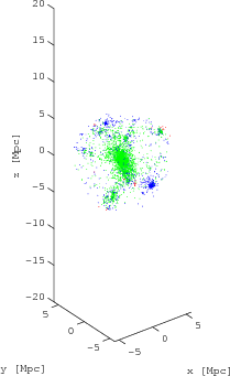
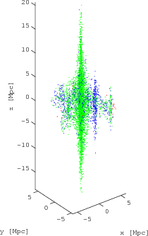
Figure 1: Three-dimensional effect of transforming to redshift space using the Hubble equivalence between velocity and distance. On the left, structure in real space. On the right, structure in redshift space. In green particles bound to the structure and in blue unbound particles. For clarity, only particles inside the critical radius in real space were plotted.

To go from the real-space to the redshift-space representation, we need to replace the coordinate along the line of sight by the corresponding recession velocity. For simplicity, we will assume that the distance to the structures is much greater than their size, so we do not need to account for angular effects and the replacement can be done directly in Cartesian space. An example of this transformation is shown in Figure 1, where the structure on the right is the redshift representation of the structure on the left, as seen by an observer looking along the $Z$ axis. In the case of a spherically symmetric structure, as described by the spherical collapse model, the projected velocity seen by an observer will be composed by the projection of the radial velocity of the spherical shell with respect to its center and the recession velocity of the whole structure (see Figure 2A).

Let us consider a spherically symmetric, gravitationally bound structure. Each shell has its own radial speed, which only depends on its enclosed density contrast. As the spherical collapse model constrains the shells not to cross each other, we will see the innermost shells falling at greater speeds than outer ones. When moving from the center to greater radii, we will cross a shell that just stopped its expansion, through slowly expanding ones, up to shells expanding with the Hubble flow. According to this model, the critical shell will be expanding with a speed (critical velocity) of only 29% of the Hubble flow at the present time (see Paper I).

We are interested in identifying all shells lying within the critical shell, each of which will have a different projected shape in redshift space. Slowly expanding shells will appear as ellipsoids shrunk along the line of sight, while fast contracting ones will appear elongated along the line of sight, but flipped, so that apparently closer points will really be at the more distant side of the structure (Kaiser, 1987). A diagram explaining this effect is shown in Figure 2, where a fast contracting shell has a higher projected velocity than the outer expanding shell, protruding from the outer ellipsoid and producing the well-known “Finger of God” effect.

We define the projected velocity envelope as the surface that encloses the redshift-space representation of all shells within a given radius $R$. This can be written as

$$v^{\mathrm{env}}_{\mathrm{p}}\left(r_{\mathrm{p}}\right)=\max_{r\in[r_{\mathrm{p}},R]}\left\{|v_{r}\left(r\right)|\sqrt{1-\left(\frac{r_{p}}{r}\right)^{2}}\right\},$$ (2)

where $v_{\mathrm{r}}$ is the radial velocity respect to the centre of the structure and $r_{\mathrm{p}}$ is the projected radius on the sky (Reisenegger et al. 2000). The spherical collapse model allows to predict $v_{\mathrm{r}}(r)$, and therefore $v^{\mathrm{env}}_{\mathrm{p}}\left(r_{\mathrm{p}}\right)$, directly from the density profile (Paper I). Setting $R$ equal to the critical radius of the structure ($r_{\mathrm{cs}}$), yields the critical projected velocity envelope (“critical envelope”, for short), corresponding to the redshift-space envelope of all shells within the critical shell. The velocity envelope, when defined up to the turn-around radius, is equivalent to the caustics defined by Regos & Geller (1989).

If all the assumptions of the spherical collapse model were true, one would expect that all the bound particles should lie within this critical envelope. Moreover, if inner ellipsoids protrude from the ellipsoid defined by the critical shell, then one would expect to see contamination in the protruding regions from objects outside the critical shell.

An effect that is not considered in the spherical collapse model are the velocity perturbations due to the interaction between nearby objects that will mix many particles into and out of the critical envelope, causing large systematic and random errors in the intended criterion for determining the limits of the bound structure in redshift space. To account for these systematic errors we used $N$-body simulations as described in the next section.

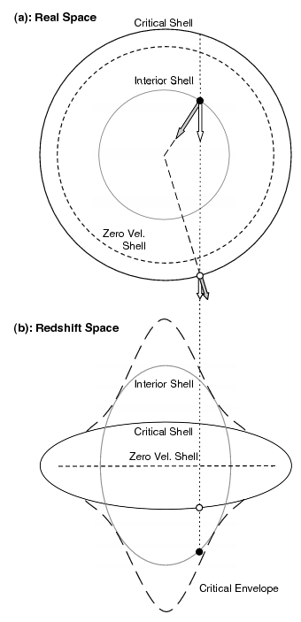
Figure 2: Redshift-space appearance of spherical shells. Panel (a) shows the position of shells in real space: the interior shell (grey) is contracting, the dashed shell is at rest, and the outer shell (black) is expanding at the critical velocity. The black dot on the contracting shell is falling faster than the expansion of the white dot on the critical shell, so its projected velocity is higher, appearing closer in redshift space. Panel (b) shows the corresponding ellipsoids in redshift space: the colouring has been kept from panel (a). The critical shell appears shrunk along the line of sight because its expansion speed is less that the Hubble flow at its radius. The interior shell instead appears elongated along the line of sight because its contraction speed is higher than the Hubble flow at its radius, but also flipped, such that the far side appears closer that the near side. The zero velocity shell appears as an horizontal line. The black long-dashed line shows the projected velocity envelope obtained from including all shells inside the critical shell.

2.2 Velocity Envelope in $N$-Body Simulations

In order to study the behaviour of structures in redshift space, we used numerical simulations, which permitted us to observe the redshift-space distribution of the structures, knowing at the same time which particles were bound and which were not. Our simulations are the same as described in Paper I, performed with the GADGET2 code (Springel, 2005), containing $128^{3}$ dark matter particles inside a box of side length $100\hbox{$\thinspace h^{-1}\hbox{$\rm\thinspace Mpc$}$}$, and considering a flat $\Lambda$CDM universe with $\Omega_{\Lambda}=0.7$. We took snapshots at the present time ($a=1$) and in the far future ($a=100$), assuming that in late epochs the structure evolution will decrease significantly so no major changes will be seen from then on (see also Busha et al. 2003 and Nagamine & Loeb 2003).

We selected the 11 largest structures for our study, with masses ranging from $1\times 10^{14}\hbox{${\rm\thinspace M}_{\sun}$}$ to $7\times 10^{14}\hbox{${\rm\thinspace M}_{\sun}$}$. Although these structures might be rather small to represent our current understanding of superclusters, many of them showed significant substructure, as expected from objects that are still evolving into a virialized state. The bound particles were identified using the state at $a=100$ and then correspondingly tagged and followed to the present frame, repeating the procedure described in Paper I.

In order to transform the simulated data to redshift space, we replaced the distance along one axis by the corresponding projected velocity. This can be done in any direction, but for simplicity we did so only along the three main axes, giving a total of 33 data sets for statistical analysis.

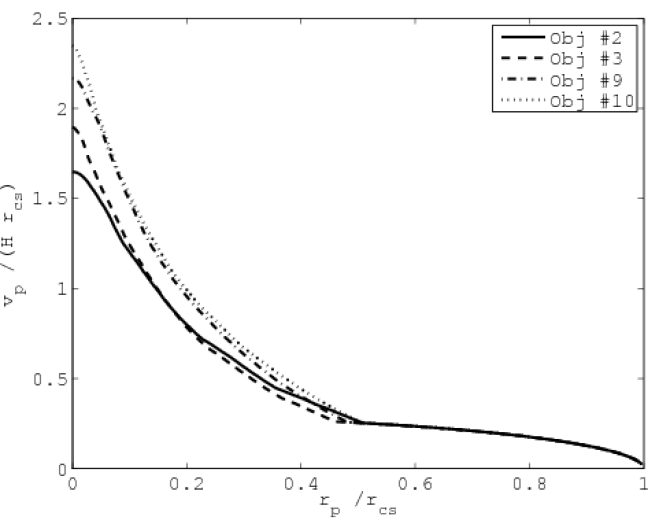
Figure 3: Critical projected velocity envelopes along the line of sight as expected in the spherical collapse model from the density profile for four well-behaved, representative simulated structures. Badly behaved structures, generally implying double cores or very significant substructure, usually present lower peak velocities and wider central regions. Radii are normalized in terms of the critical shell’s radius and velocities in terms of the Hubble flow at that radius. The masses satisfy $M_{\mathrm{obj\#2}}>M_{\mathrm{obj\#3}}>M_{\mathrm{obj\#9}}>M_{\mathrm{obj\#10}}$ (see Table 3).

Figure 3 shows the critical envelope for two objects in our study with nearly spherical symmetry, with radii normalized in terms of the critical radius $r_{\mathrm{cs}}$ and velocities referred to the Hubble flow at $r_{\mathrm{cs}}$. These critical envelopes were obtained measuring the density contrast at all radii and applying the procedure described in Paper I to find the radial velocity, and finally projecting it along the line of sight. At large radius, where there is no ellipsoid crossing, we see the ellipsoid corresponding to the critical shell, which has the same shape since its expansion velocity is the same fraction ($29\%$ in present time) of the Hubble flow (see Paper I). At smaller radius we observe the existence of ellipsoid crossing in redshift space, which is produced because the inner shells are contracting faster than the expansion velocity of the critical shell. Adjusting the object’s centre, we observe an improvement in matching the resulting profiles. Specifically, a choice closer to the densest core of the structure increases the height of the peak of the velocity envelopes and improves the agreement between the shapes of curves corresponding to different objects. Even though the profiles do not match exactly at small radii, all of them share the same characteristic shape, showing higher velocities in less massive objects, meaning a higher concentration than more massive structures, in qualitative agreement with the results of Navarro, Frenk & White (1997). These properties suggest that it may be possible to estimate the critical envelope by a general template that depends only on the bound mass of the structure.

To study the accuracy of the prediction given by the critical envelope for the location of particles in redshift space, we counted the number of bound particles inside and outside the critical envelope, as well as the number of unbound particles inside the critical envelope. Our results are summarized in Table 1. We used the same statistical indicators as in Paper I, so now we can compare the performance of the criteria in redshift and real spaces. The indicators, all expressed as percentages of the total number of particles inside the critical envelope, are:

• $A$: particles inside the critical envelope that do not belong to the cluster at $a=100$.

• $B$: particles inside the critical envelope that do belong to the cluster at $a=100$.

• $C$: particles outside the critical envelope that belong to the cluster at $a=100$.

• $D$: all particles that belong to the cluster at $a=100$.

Note that $A+B$ = 100% and $D=B+C$.

Table 1: Mean values and standard deviations for several performance indicators for the critical envelope corresponding to the true density profile (see text).

	Redshift Space		Real Space
Indicator	Mean	Std. Dev	Mean	Std. Dev
$A$	23.96	10.01	28.2	13.0
$B$	76.04	10.01	71.8	13.0
$C$	30.59	13.24	0.26	0.23
$D$	106.62	17.56	72.0	13.1

We observe that, compared to the real-space criterion (Paper I), the new redshift-space criterion produces better results for the indicators $A$ and $B$, but the indicator $C$ increases significantly (see Table 1), implying that it does not give an external limit to the location of particles in redshift space, in contrast with the real-space case.

As pointed out before, compared to predictions done in real space, predictions done on redshift space are affected by a higher mixing of bound and unbound particles. This is due to the velocity dispersion, which makes many particles (inside the critical shell in real space) fall outside of the critical envelope in redshift space. The velocity dispersion is produced by local interactions between nearby objects as they decelerate driven by the central attractor, manifesting as local peculiar velocities in random directions. To check if the velocity dispersion was accompanied by an increase in the mean speed of the particles (as expected), we plotted the later with respect to their radii, comparing it to the absolute value of the theoretical radial velocity profile.

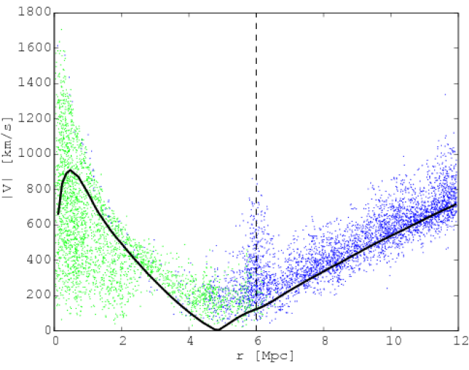
Figure 4: Absolute value of the velocities versus their radii to the centre for Obj. #9. The solid line shows the absolute theoretical velocity. The dashed line indicates the critical radius. The turn-around radius is clearly observed where the solid line touches zero, accompanied, as expected, by a minimum of absolute velocities. For clarity we plotted a 70% random sample of all particles.

In Figure 4, we can see how the theoretical profile approximately marks the lower bound of absolute velocities for particles inside the critical radius, but outside the virialized core (around $2.5\hbox{$\rm\thinspace Mpc$}$ from the centre), so we can claim that the main contributor for particles escaping from the critical envelope is the overall increment in particle speeds due to interactions between them.

2.3 Density Profile Template

Until now, we have used the measured density profile to estimate the critical envelope from our simulated structures. When confronted with observational data in redshift space, we will not have this information, so we need a general way to estimate the density profile of a structure based on a small number of parameters. We have seen in §2.2 that the critical envelopes for different structures have a coherent shape (see Fig. 3), but with scales correlated with the bound mass of the structure. This is in agreement to what was proposed by Navarro, Frenk & White (1997), who presented the now well-known NFW profile, which is a generalized density profile for virialized clusters, obtained empirically from many simulations. In particular, we used the results from a later publication (Eke, Navarro, & Steinmetz 2001), which corrected several details from the original work. In general words, they postulate that a cluster’s density profile can be estimated using as a single parameter, the radius $r_{\Delta}$ at which a characteristic (“virial”) density contrast $\Delta$ is reached. The parameter $\Delta$ depends on the cosmology and can be obtained in a flat universe as $\Delta=178\Omega_{\mathrm{m}}^{0.45}$, which in our case gives $\Delta=103.5$. This characteristic radius is much smaller than our critical radius, falling near the edge of the virialized zone where clusters are less affected by external structures and look more homogeneous, making it easier to estimate using redshift data. The NFW profile was formulated to give good results for radii ranging from $0.1r_{s}$ to $10r_{s}$, where $r_{s}=r_{\Delta}/\mathrm{c}_{\Delta}$ and $c_{\Delta}$ is the concentration parameter, which can be obtained as a function of the mass contained within $r_{\Delta}$, and whose value is around $\sim 8$ for the masses of the structures studied by us. Considering that the critical radius is of order $3-5r_{\Delta}$, the NFW profile is more accurate for the inner part of the structure. This region is the most interesting one for our purposes, since it is where ellipsoid crossing takes place and the shape of the critical envelope is directly dependent on the density profile. On the other hand, we caution that large bound structures may generally not be dominated by clusters as relaxed and spherical as those for which the NFW profile was derived.

The NFW density profile was fitted to every object in our simulation using the actual density in real space.

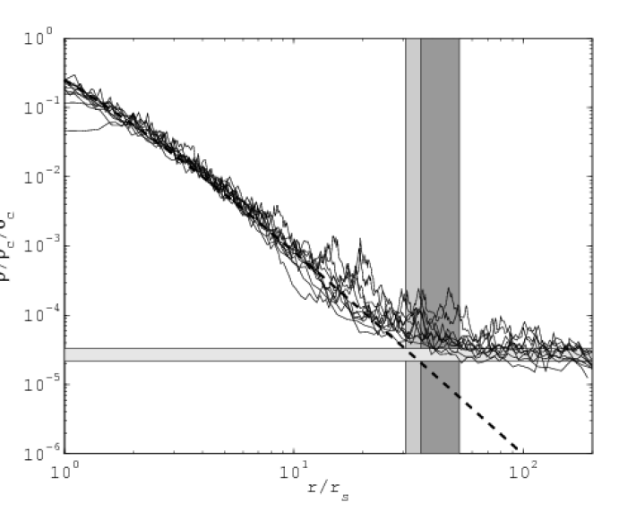
Figure 5: Density profiles of all structures (solid), compared to the NFW template (dashed). The densities and radii have been normalized by their corresponding scale in the NFW template to put them on the same plot. The dark and light grey vertical areas denote placement of critical radii measured from the simulated data and from the fitted NFW template respectively (the dark grey area actually extends under the light grey area up to its left end, but is hard to see in the plot). The horizontal area denotes the range for the asymptotic values for the density, $\Omega_{\mathrm{m}}\rho_{\mathrm{c}}$.

Figure 5 shows the density profiles for all our simulated structures, compared to the NFW template profile. Scales have been normalized by their corresponding NFW scale, in order to let us compare all profiles to a single NFW template. The dark and light grey vertical areas show where the critical radii obtained from the simulated data and from the NFW profile, respectively, are located. The horizontal area shows the asymptotic values expected as the density reaches the mean density of the Universe. Clearly, the true density profiles depart from the template at radii somewhat smaller than the critical radius, as they approach the mean density of the Universe. This early departure from the model implies that estimation of the critical radius done directly from the NFW template will be biased to lower values. Below, we will present ways to deal with this bias.

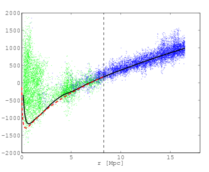
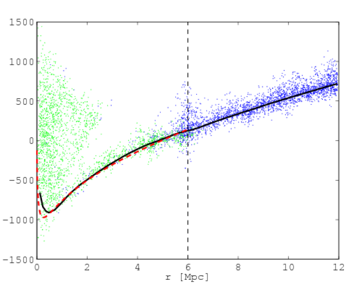
Figure 6: Radial velocities compared to the theoretical velocity profile obtained from the true density profile (black solid line) and from the NFW density profile fitted to the structure (red dashed line). Green dots indicate bound objects and blue dots the opposite. On the left object #1, and on the right object #9. Sampling 50%.

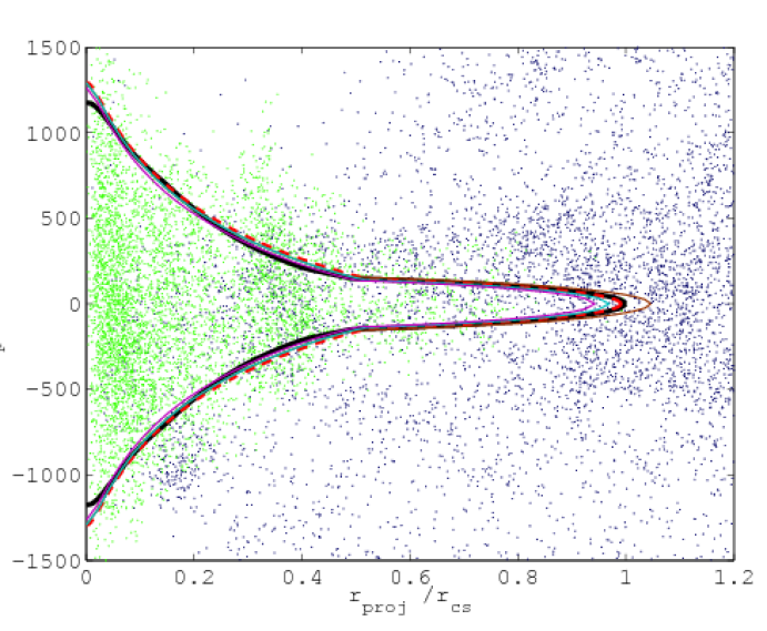
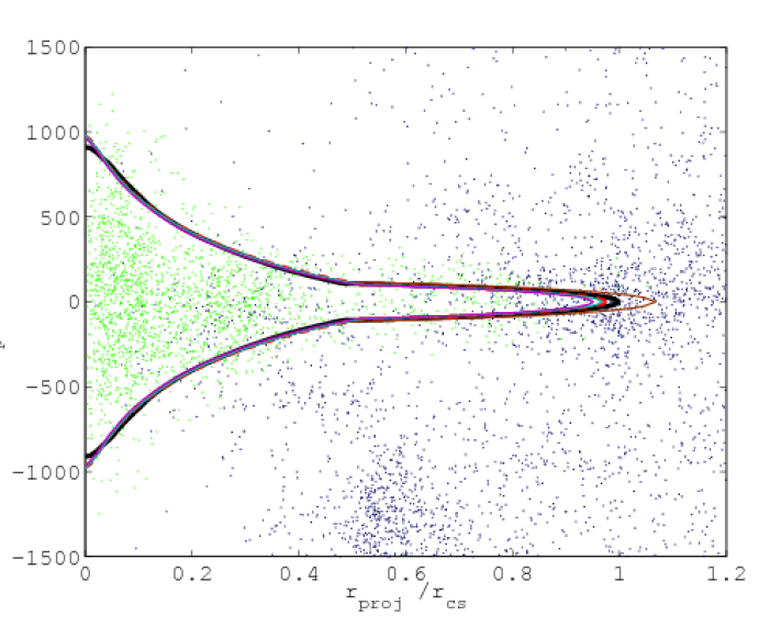
Figure 7: Projected velocities versus normalized projected radius. In green, particles that will eventually fall in the object. In blue, particles that will escape. The curves show different critical envelope estimations: The black solid line shows the true velocity envelope. The red dashed line is the NFW envelope adjusted using the observed $r_{\Delta}$ value. The cyan solid line is the NFW envelope fitted using the NFW-core method (fitting methods are explained in §3.2). The magenta solid line is the NFW envelope fitted using the NFW-cs method. The brown solid line show the combined envelope fitted using the combined method. On the left object #1, and on the right object #9. Sampling 50%.

As seen in Figures 6 and 7, the radial velocities and critical envelopes predicted using a NFW density profile show different levels of agreement with the true velocities depending on the range of radii considered. For small radii, it yields a higher density than observed, predicting higher infall velocities. Given the resolution of our simulation, which was intended to search for large scale structure rather than replicating the behaviour of the virialized cores of structures, we believe that our simulated data is unable to produce accurate densities at such radii. For intermediate radii, the prediction is very good, as expected, since the NFW profile was fitted at a measured $r_{\Delta}$ in this range. Finally, for larger radii, closer to $r_{\mathrm{cs}}$, the generalized profile gives better or worse results depending on the absence or presence of significant substructure, respectively. In general, the presence of substructure increases the density at higher radii, so the NFW profile underestimates it, consequently giving a low estimate for the critical radius.

Table 2: Critical radii considering different models in real space. Columns: (1) Object index. (2) $r_{\Delta}$: virialization radius needed to fit the NFW density profile. (3) $r_{\mathrm{cs}}$: critical radius applying to our criterion ($\Omega_{\mathrm{cs}}=2.36$) to the true density profile. (4) $r_{\mathrm{cs}}^{\mathrm{NFW}}$: critical radius applying our criterion to the fitted NFW profile ($\Omega_{\mathrm{cs}}^{\mathrm{NFW}}=2.36$). (5) Ratio between $r_{\mathrm{cs}}^{\mathrm{NFW}}$ and $r_{\mathrm{cs}}$.

Obj.#	$r_{\Delta}[Mpc]$	$r_{\mathrm{cs}}[Mpc]$	$r_{\mathrm{cs}}^{\mathrm{NFW}}[Mpc]$	$r_{\mathrm{cs}}^{\mathrm{NFW}}/r_{\mathrm{cs}}$
1	1.81	8.28	8.21	0.99
2	1.51	7.84	6.79	0.87
3	1.48	7.54	6.65	0.88
4	1.56	7.92	7.02	0.89
5	1.30	7.38	5.80	0.79
6	1.21	7.93	5.38	0.68
7	1.48	7.63	6.64	0.87
8	1.30	6.29	5.80	0.92
9	1.31	6.01	5.85	0.97
10	1.27	5.67	5.66	1.00
11	1.23	5.37	5.49	1.02

Table 3: Enclosed masses considering different models in real space, contrasted to the effectively bound mass. Columns: (1) Object index. (2) $M_{\mathrm{bound}}$: Bound mass at a = 100. (3) $M_{\mathrm{cs}}$: Mass enclosed by the critical radius $r_{\mathrm{cs}}$. (4) Mass ratio between bounded mass and $M_{\mathrm{cs}}$ (5) $M_{\mathrm{cs}}^{\mathrm{NFW}}$: Mass enclosed by the critical radius obtained using the NFW density profile $r_{\mathrm{cs}}^{\mathrm{NFW}}$. (6) Mass ratio for $M_{\mathrm{cs}}^{\mathrm{NFW}}$.

Obj.#	$M_{\mathrm{bound}}$	$M_{\mathrm{cs}}$	$\frac{M_{\mathrm{bound}}}{M_{\mathrm{cs}}}$	$M_{\mathrm{cs}}^{\mathrm{NFW}}$	$\frac{M_{\mathrm{bound}}}{M_{\mathrm{cs}}^{\mathrm{NFW}}}$
1	6.34	7.64	0.83	7.60	0.83
2	5.29	6.47	0.82	5.96	0.89
3	4.71	5.76	0.82	5.26	0.90
4	4.14	6.68	0.62	5.99	0.69
5	4.07	5.41	0.75	4.31	0.94
6	3.23	6.70	0.48	3.01	1.07
7	2.95	5.98	0.49	4.53	0.65
8	2.44	3.34	0.73	3.18	0.77
9	2.40	2.91	0.83	2.79	0.86
10	2.02	2.45	0.82	2.44	0.82
11	1.46	2.08	0.70	2.18	0.67
All masses in units of $10^{14}\hbox{${\rm\thinspace M}_{\sun}$}$

Tables 2 and 3 compare the predicted critical radius and enclosed mass for every object in the analysis. We observe that the critical radius according to the NFW profile is 89.8% of the measured critical radius. Thus, considering that the spherical collapse criterion gives an external limit for the critical radius, estimations done with the NFW profile will underestimate the size of the structure as defined by the spherical-collapse criterion.

Concerning the mass of the structures, we find that the mean true bound mass ($M_{\mathrm{bound}}$) is 82.7% of the mass enclosed by the NFW profile critical radius in real space. This should be compared to the same relation for the true critical radius, where the true bound mass is 71.7% of the mass enclosed by it (see Paper I for details).

3 Fitting Method Definition

3.1 Density Estimator

The great advantage of using the NFW profile is that the resulting critical envelope depends exclusively on the bound mass of the studied structure. In this way, the projected velocity envelope can be scaled (changing either $r_{\Delta}$ or $M_{\Delta}$) until the contained mass and volume satisfy some condition equivalent to the critical density contrast, but in redshift space. For this purpose, we will define an observable to characterize the redshift-space density contrast inside the surface given by a certain projected velocity envelope. The redshift-space “density estimator” is defined as

$$\hat{\Omega}_{\mathrm{R}}=\frac{\hat{M}_{\mathrm{R}}}{V_{\mathrm{R}}\rho_{\mathrm{c}}},$$ (3)

where $\hat{M}_{\mathrm{R}}$ is the mass inside the projected velocity envelope defined by the radius $R$ and $V_{\mathrm{R}}=4\pi R^{3}/3$ is the real-space volume enclosed by the same radius. This definition allows us to obtain density estimators for any projected velocity envelope, including the critical envelope. In practice we will need to define density estimators for only two kinds of projected velocity envelopes: the critical envelope and the “core envelope”, which is the projected velocity envelope obtained using the NFW density profile for radii within $r_{\Delta}$, necessary to estimate the NFW density profile in redshift space. These density estimators can be computed for all the structures in our sample, and then averaged to produce a calibrated estimator that can let us infer the correct critical envelope without need of real-space data.

The aim is to have a general template for the desired projected velocity envelope, which can be associated to a specific density estimator, specially calibrated for it. When fitting a template to data from a redshift survey, it can be scaled until its density estimator takes the desired value, yielding an estimation for the radius in real space that characterises it.

To understand better the properties of the density estimator, we calculated it using the “true critical envelope” (infered from the true density obtained from the simulations) from all our 11 objects from 3 points of view. Results are shown in Table 4. The mean value for the density estimator is $\hat{\bar{\Omega}}_{\mathrm{cs}}=1.60$. This value is significantly lower than the criterion $\Omega_{\mathrm{cs}}=2.36$ for real space, implying that the selected volume is less populated or, in other words, many more particles escaped the theoretical prediction, also reflected in the greater value for $C$. This leads to the conclusion that perturbations away from the spherical collapse model have a stronger manifestation in particles velocities than in their positions, decreasing the reliability of predictions in redshift space.

Table 4: Density estimators for all projections. Rows: (1 - 3) Projections in the $x$, $y$ and $z$ axes. (4) Mean values for each object. Columns: All 11 objects.

Object	#1	#2	#3	#4	#5	#6	#7	#8	#9	#10	#11
$x$ axis	1.92	1.48	1.65	2.16	1.23	1.30	1.43	1.84	1.77	1.68	1.68
$y$ axis	1.54	1.81	1.63	1.62	1.34	1.20	1.37	1.50	1.77	1.81	1.67
$z$ axis	1.55	1.58	1.76	1.45	1.40	1.12	1.53	1.49	1.84	1.83	1.87
Mean	1.67	1.62	1.68	1.74	1.32	1.20	1.44	1.61	1.79	1.77	1.74

3.2 Critical Envelope Recipes and Fitting Method

We would like to replace the true density profiles (unknown in actual observed structures) by a simple parametrisation, based on the NFW density profile. In order to test its accuracy, we compare the previously defined performance indicators for the following three projected velocity envelopes:

• True envelope: The projected velocity envelope is determined directly from the true density profile.

• NFW envelope: The virialization radius $r_{\Delta}$ is determined using the appropriate over-density criterion in real space, yielding an NFW density profile, which is used to generate a projected velocity envelope defined for shells within the critical radius according to the NFW density profile.

• Combined envelope: $r_{\Delta}$ and $r_{\mathrm{cs}}$ are found using the appropriate over-density criteria in real space. We generate a projected velocity envelope using the ellipsoid corresponding to the critical shell, adding the inner part of the NFW envelope where it protrudes from the ellipsoid.

Table 5 gives a comparison of the statistical indicators for all the three critical envelopes in consideration. We clearly see how the combined envelope shows almost the same statistical properties as the true envelope. In contrast the NFW envelope shows a greater amount of particles that escaped the profile (Indicator $C$).

Table 5: Mean values and standard deviations for several performance indicators for three critical envelopes obtained from real-space measurements. Rows: (1) True: Critical envelope calculated using the true density profile. (2) NFW: Uses the NFW density profile according to $r_{\Delta}$ in real space. (3) Comb: Uses the NFW profile for the innermost radii and the maximum ellipse given by the critical radius.

Envelope	$\bar{A}$	$\sigma_{A}$	$\bar{B}$	$\sigma_{B}$	$\bar{C}$	$\sigma_{C}$	$\bar{D}$	$\sigma_{D}$
True	23.96	10.01	76.04	10.01	30.59	13.24	106.62	17.33
NFW	19.72	7.35	80.28	7.35	37.17	21.67	117.42	24.23
Comb	23.88	9.98	76.12	9.98	30.80	14.09	106.93	17.55

Until now, the projected velocity envelopes have been determined from information in real space that is not available in actual observed structures. To fit the velocity envelopes directly in redshift space, we will need to use density estimators in order to scale the templates up to the desired size. Here we propose three ways to do this.

The first way is to directly try to estimate the NFW density profile for the structure, for which one needs to estimate the virialization radius $r_{\Delta}$. In order to estimate $r_{\Delta}$ from the redshift space data, we defined another template based on the NFW density profile:

• Core envelope: equivalent to the NFW envelope, but now considering only shells inside the virialization radius.

Then we can construct a density estimator $\hat{\Omega}_{\mathrm{core}}^{\mathrm{NFW}}$ that can be used to fit the core envelope in redshift space. Once we have estimated $r_{\Delta}$, we can use it for estimating $r_{\mathrm{cs}}^{\mathrm{NFW}}$, defined as the radius where the density contrast in real space $\Omega_{\mathrm{s}}^{\mathrm{NFW}}=2.36$. We labeled this recipe as “NFW-core”.

The second way is to directly fit the NFW envelope, which is defined up to $r_{\mathrm{cs}}^{\mathrm{NFW}}$, using a density estimator previously calibrated for this template ($\hat{\Omega}_{\mathrm{cs}}^{\mathrm{NFW}}$). The fitted envelope will directly estimate the critical radius $r_{\mathrm{cs}}^{\mathrm{NFW}}$. We labeled this recipe as “NFW-cs”.

The last method is to use the combined envelope, for which we need to estimate two independent parameters, $r_{\Delta}$ and $r_{\mathrm{cs}}$. For the first we can fit the core envelope, following the same procedure as in the NFW-core recipe. After estimating $r_{\Delta}$, we can construct the combined envelope leaving as a single free parameter the critical radius $r_{\mathrm{cs}}$, which defines the outer ellipsoid. Finally we can use another density estimator, $\hat{\Omega}_{\mathrm{cs}}^{\mathrm{comb}}$, previously calibrated for the combined envelope, to fit this last parameter. We labeled this recipe as “comb”.

Having estimated the critical radius using one of these methods, we use equation (1) to estimate the enclosed mass. Then the true bound mass can be estimated using the statistical relation between the mass inside the critical shell and the bound mass, as explained in Paper I.

3.3 Centre Determination

A very important step in our method for identifying the structure limits is to first have a good estimate for its centre, where to anchor the projected velocity envelope. The intuitive way to do this is to look for the region with the highest density of particles (galaxies) in redshift space. In other words, we need to find the centre which maximises the size of the projected velocity envelope for a given density estimator. We performed this maximisation using the core envelope, focusing on finding the densest virialized centre for our structure. As density estimator we used $\hat{\Omega}_{\mathrm{core}}^{\mathrm{NFW}}$ calibrated for the centre found in real space, using the procedure described in the next subsection.

We found that the new centre appeared to be displaced from the original centre on average a 13.5% of $r_{\Delta}$ (representing the virialized core), but the errors produced from using this new centre were marginal compared to other systematic errors, being around one order magnitude smaller.

3.4 Density Estimator Calibration

In order to use the general projected velocity envelope to estimate the critical radius of gravitationally bound structures, we first need to obtain a density estimator specially calibrated for that particular type of projected velocity envelope. The best way of doing this is to use a statistically significant number of simulated structures in the scale range we are interested in, and calculate the corresponding density estimator using the actual projected velocity envelope obtained from real-space measurements.

Here, we are going to use the mean of the density estimators found in all 33 projections as our calibrated density estimator, and the standard deviation will be used as the expected error. The density estimators needed by our projected velocity envelope recipes are $\hat{\Omega}_{\mathrm{core}}^{\mathrm{NFW}}$ for the core envelope, $\hat{\Omega}_{\mathrm{cs}}^{\mathrm{NFW}}$ for the NFW envelope and $\hat{\Omega}_{\mathrm{cs}}^{\mathrm{comb}}$ for the combined envelope.

The mean density estimators, together with their standard deviations are shown in Table 6. For completeness, and as a comparison point, we also included the mean density estimator for the true envelope, $\hat{\Omega}_{\mathrm{cs}}^{\mathrm{true}}$, which can also be found for every single object and point of view in Table 4.

Table 6: Mean values and standard deviations for inner density estimators for several projected velocity envelopes with parameters determined in real space. See row definitions in the text. The first three estimators correspond to envelopes defined up to the critical radius, while the forth is defined up to the much smaller virialization radius $\mathrm{r_{\Delta}}$.

Envelope	Estimator	Mean	Std. Dev.
True	$\hat{\Omega}_{\mathrm{cs}}^{\mathrm{true}}$	1.59	0.25
NFW	$\hat{\Omega}_{\mathrm{cs}}^{\mathrm{NFW}}$	2.06	0.35
Comb	$\hat{\Omega}_{\mathrm{cs}}^{\mathrm{comb}}$	1.59	0.26
Core	$\hat{\Omega}_{\mathrm{core}}^{\mathrm{NFW}}$	109.64	14.56

We observe that the True and Combined density estimators are very similar, which tells us that the NFW profile accurately reproduces the central part of the true velocity envelope. On the other hand, the NFW envelope has a much greater density estimator, which is the result of a smaller critical radius ($r_{\mathrm{cs}}^{\mathrm{NFW}}$). The density estimator associated to the core envelope is actually very close to its equivalent value in real space ($\Delta=103.5$), which is good considering that the structures’ core are ruled by virialization, far from the spherical collapse constraints we are assuming.

3.5 Main Sources of Error

We can distinguish two kinds of error sources when first looking at Table 4: the first is associated to big variability in the estimator depending on the axis being viewed, and the other is manifested as an overall under or overestimation of the density estimator for all views of the same object. For the first, the axis dependence tells us that there is a strong influence of the cluster’s particular geometry or anisotropies outside of the spherical distribution. A good example is Obj.# 4, where we find a big deviation in observations done along the $X$ axis, showing an overestimation of the inner density with respect to observations done along the other axes. After analyzing the statistics, and plotting the radial velocities from all axes (see Figure 8), we conclude that this difference is produced by an inflow of particles from an external structure placed right on the line of sight, and whose virialized velocities mix in redshift space with particles from the studied cluster. The effect is an oversized parameter $A$ and an undersized parameter $C$.

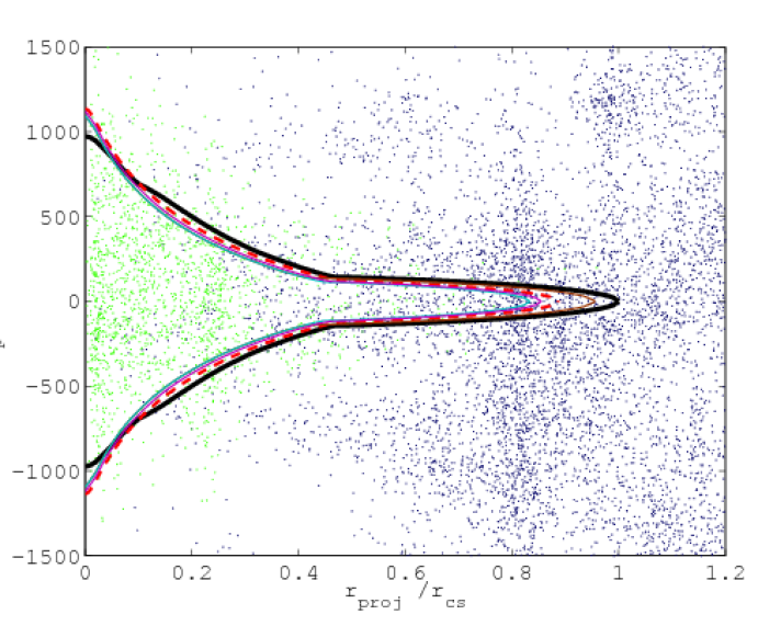
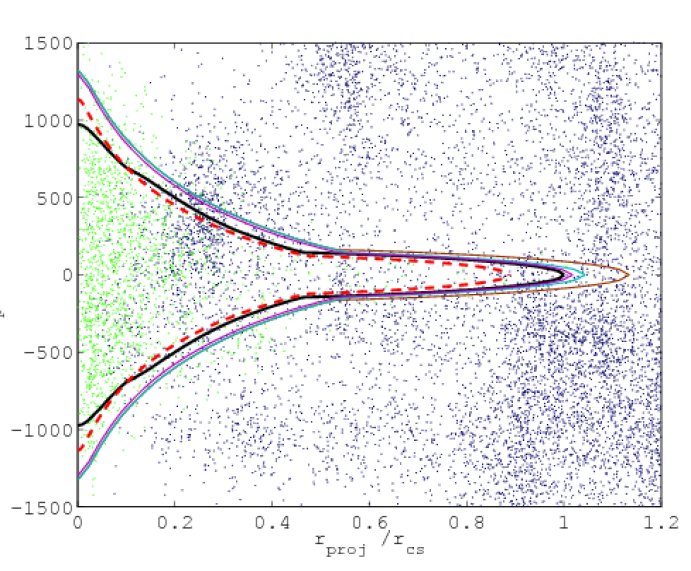
Figure 8: Projected velocities versus normalized projected radius for Obj#4. On the left is the $X$ axis view, while on the left is the $Y$ axis view. Sampling 50%.

These observations appeared repeated in every object with big standard deviation of the density estimator among the three axes, but did not appear related to objects with highly non-spherical cores or double cores.

Regarding the second type of error, we conclude that it is related to highly non-spherical cores or anisotropies inside the critical radius. That is the case of Obj.#5 shown in Figure 9, which has a double core. We observe that the double core does not produce a big deviation between estimations from different axes, but produces a significant underestimation of the inner density, which at the end will cause that this kind of objects will be bigger than predicted.

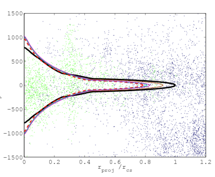
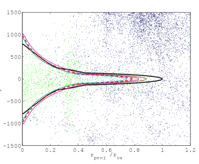
Figure 9: Projected velocities versus normalized projected radius for Obj#5. This object presents a double core that will eventually merge into a single object. We observe that this feature does not produce a significant effect when observing it from a different point of view. Sampling 50%.

4 Fitting Method Testing

Before being able to apply the method to real observations, we tested it in our simulations, in order to get statistical information that can be used to interpret later results.

4.1 Performance Statistics

We fitted the three kinds of critical envelopes to our data in redshift space using our previously calibrated density estimators. Considering that we have only 11 objects in our study, we decided to use the same data to do the fittings, but we rotated the redshift projections in $45^{\circ}$ to at least use different points of view at this stage. To fit the profiles, we just scaled them until the density estimator condition was reached. As centre for the profiles, we used our redshift-determined centres. We realized three fittings:

• Combined method (comb): Uses the density estimator $\hat{\Omega}_{\mathrm{core}}^{\mathrm{NFW}}$ to fit the core envelope and calculate $r_{\Delta}$. Then fits an ellipsoid (that corresponds to the critical shell) adjusting its radius until the combined envelope produce the desired density estimator, $\hat{\Omega}_{\mathrm{cs}}^{\mathrm{comb}}$, directly estimating $r_{\mathrm{cs}}$.

• NFW-based method (NFW-core): Uses the density estimator $\hat{\Omega}_{\mathrm{core}}^{\mathrm{NFW}}$ to fit the core envelope and calculate $r_{\Delta}$. Then uses the NFW density profile to calculate the critical radius $r_{\mathrm{cs}}^{\mathrm{NFW}}$.

• NFW-based method 2 (NFW-cs): Uses the density estimator $\hat{\Omega}_{\mathrm{cs}}^{\mathrm{NFW}}$ to fit the whole NFW envelope to the structure in redshift space, directly estimating $r_{\mathrm{cs}}^{\mathrm{NFW}}$.

For the radius and mass estimations, we need to consider the systematic biases discussed in subsection 2.3 for the critical radius obtained from the NFW density profile $r_{\mathrm{cs}}^{\mathrm{NFW}}$ and for the bound mass estimated from the mass enclosed by the critical radius. In particular we use that $\hat{r}_{\mathrm{cs}}=r_{\mathrm{cs}}^{\mathrm{NFW}}/0.898$ and $\hat{M}_{\mathrm{bound}}=0.717\hat{M}_{\mathrm{cs}}$, where $\hat{M}_{\mathrm{cs}}$ is the mass derived from equation (1).

There are two main statistics we are interested in: The first denotes mean systematic deviations of the estimated parameter (radius or mass) from the true value. For this we define the parameter $\alpha_{\mathrm{i}}$ as the mean of the ratio between the estimated and the true value of the physical property $i$. The existence of this kind of mean biases is mostly due to statistical deviations, and should disappear as we increase the number of structures studied for the whole calibration and testing of this system.

In second place we are interested in quantifying errors due to morphological characteristics that depart individual structures from the mean. A way to do this is calculating the standard deviation of measurements done from different angles, normalised by the true value, which has the advantage of discounting the mean bias produced by systematic errors. We labelled this as $\sigma_{x,i}$, where $i$ denotes again the physical property we are referring to. The mean parameter, averaged over all structures, $\bar{\sigma}_{x}$, will give us the error we expect to find in estimations done without taking into consideration the particular morphological properties of the studied structure.

Table 7: Systematic bias errors and mean standard deviation. Columns: (1): Fitting method. (2), (4) and (6): Mean normalised bias $\bar{\alpha}$ in the measured $r_{\Delta}$, $r_{\mathrm{cs}}$ and $M$. (3), (5) and (7): standard deviation $\bar{\sigma}_{x}$, which represents the deviation of estimations along different axes with respect to the mean of the estimations for the same object.

Method	$\bar{\alpha}_{\Delta}$	$\bar{\sigma}_{x,\Delta}$	$\bar{\alpha}_{c}$	$\bar{\sigma}_{x,c}$	$\bar{\alpha}_{M}$	$\bar{\sigma}_{x,M}$
Comb	1.013	0.080	1.000	0.068	1.045	0.206
NFW1	1.013	0.080	1.007	0.083	1.086	0.253
NFW2	1.015	0.066	1.003	0.068	1.055	0.203

The mean results from this analysis can be found in Table 7. There we can observe that the systematic biases are all very small, reaching in the worst cases 1.5% for $r_{\Delta}$ estimations, 0.7% for $r_{\mathrm{cs}}$ estimations and 8.6% for mass estimations. This result should be taken with some care, because we need to consider that there is an evident correlation between the source and the test data for our system, but this situation can be improved very easily by growing our sample with new simulated structures.

For the standard deviation, we observe that errors due to morphological anisotropies out of the spherical symmetry reach in the worst cases 8.0% for $r_{\Delta}$ estimations, 8.3% for $r_{\mathrm{cs}}$ estimations and 25% for mass estimations.

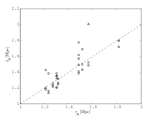
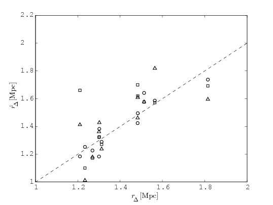
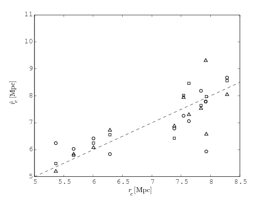
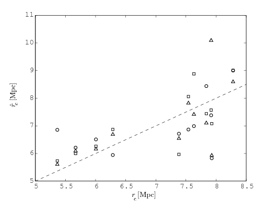
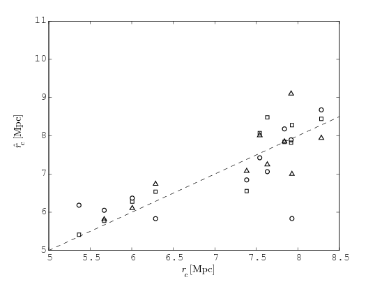
Figure 10: Estimated virial radii $r_{\Delta}$ versus measured virial radii for all profile recipes and points of view. On the left, results from the combined method. In the centre, results from NFW-core method. On the right, results from NFW-cs method. Circles indicate $X$-axis projections, triangles indicate $Y$-axis projections and squares indicate $Z$-axis projections.

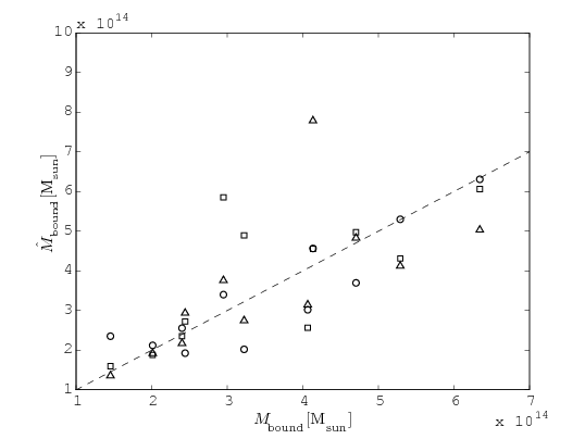
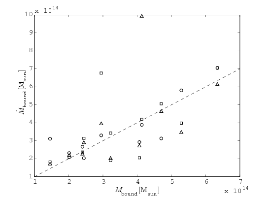
Figure 11: Estimated critical radii versus measured critical radii for all profile recipes and points of view. On the left, results from the combined method. In the centre, results from NFW-core method. On the right, results from NFW-cs method. Circles indicate $X$-axis projections, triangles indicate $Y$-axis projections and squares indicate $Z$-axis projections. Results have been debiased considering that $r_{\mathrm{cs,NFW}}=0.898r_{\mathrm{cs}}$

Figure 12: Estimated bound masses versus measured bound masses (in $a=1$). On the left, results from the combined method. In the centre, results from NFW-core method. On the right, results from NFW-cs method. Circles indicate $X$-axis projections, triangles indicate $Y$-axis projections and squares indicate $Z$-axis projections. Results have been debiased considering that $r_{\mathrm{cs}}^{\mathrm{NFW}}=0.898r_{\mathrm{cs}}$ for the NFW-based methods and $M_{\mathrm{bound}}=0.717M_{\mathrm{cs}}$ for all.

In Figures 12, 12 and 12, we present the results for all methods. It is clear that the method is axis-dependent, showing big deviations in structures with strange morphologies. These deviations are in agreement with the variability observed in the density estimators shown in Table 4, suggesting that much can be done identifying types of structures and calibrating custom density estimators for them.

As a last conclusion, we observe that the best results are obtained with the combined and NFW-cs methods, both of which have in common that they are fitted to $r_{\mathrm{cs}}$ instead of $r_{\Delta}$.

4.2 Error Estimation

The most direct way to estimate the expected error from estimating the size and mass of a bound structure using this method is to calculate the actual deviations from the true value over all objects in our study. For the critical radius and the bound mass we used the following equation:

$$Err_{x}=\sqrt{\frac{1}{N}\sum_{i}\frac{\left(\hat{x}_{i}-x_{i}\right)^{2}}{x_{i}^{2}}},$$ (4)

where $x$ is the parameter on which we want to determine the error.

Table 8: Expected errors in critical radius and bound mass estimations. Columns: (1): Fitting method. (2): Percentage error in critical radius estimation. (3): Percentage error in bound mass estimation.

Method	$Error_{r}$%	$Error_{M}\%$
Comb	8.5	31.3
NFW1	12.2	44.1
NFW2	8.1	30.9

The expected errors calculated in this way are shown in Table 8. We emphasise that these errors are the ones we should expect after a “brute-force” application of the method, having no consideration of the observable morphology of the structure. Due to the statistical nature of the fitting method, one would expect significant improvement in the expected errors after a more careful analysis of individual cases, where different “kinds” of structures, including structures with evident double cores or highly contaminated by substructure, were considered. This analysis is beyond the scope of this work, but can be included in future works.

5 Conclusions

We have presented a new method to estimate the mass and radius of gravitationally bound structures based solely on redshift information present in redshift survey catalogs. The method is based on the spherical collapse model (Paper I) and on the important observation that the theoretical critical envelope correctly follows the true critical envelope deep inside the virialized centre of the simulated structures. We used the NFW density profile (Navarro, Frenk & White, 1997) to generate a template for the critical envelope, which was calibrated using $N$-body simulations.

The extension of the method to redshift space gave birth to a new set of criteria that we called “density estimators”. These were defined as the expected redshift-space density inside the projected velocity envelope. Their calculation was completely empirical, depending on statistical analysis of simulated structures due to the considerable velocity dispersion found in them. We observed that the main cause of velocity dispersion was the gain of peculiar velocities due to local interaction between in-falling objects and substructure. The study of substructure and of the morphology of the studied structure can be of great help to improve the error bars, since the density estimators show great dependence on these properties. From this, we conclude that numerical simulations can be used to emulate the particular properties of the studied structures, producing “custom-made” methods to obtain the best results.

In contrast to the caustic method, our method forces a limit to the radius of the structure, defined as the maximum radius at which one should expect to find bound objects. The shape of the velocity envelope though is less flexible than the caustics shape, suggesting that a combination of both methods can give better results, finding the envelope at lower radii using the caustics where they are more defined, and using the fixed envelope at higher radii to set a limit to the structure.

The more reliable methods from the study were the “combined” and the “NFW-cs” methods. The procedure to apply the combined method to a redshift data set is then the following:

• Calibrate data so that every element is accurately related to a mass, so that the whole data set serves as a redshift-space mass field.

• Identify the center of the structure by maximising the number of particles inside the core envelope for a given density estimator.

• Fit the NFW profile to the central region (core) by adjusting $r_{\Delta}$ until the measured density estimator is equal to the mean density estimator for the core, given in Table 6.

• Add the ellipsoid given by $r_{\mathrm{cs}}$ to the critical envelope, and adjust $r_{\mathrm{cs}}$ to the value $\hat{r}_{\mathrm{cs}}$, at which the density estimator inside the total critical envelope is equal to the mean density estimator for the combined method, given in Table 6.

• Given $\hat{r}_{\mathrm{cs}}$, calculate the bound mass using equation 1.

• The fractional errors for $\hat{r}_{\mathrm{cs}}$ and $\hat{M}_{\mathrm{bound}}$ are given in Table 8.

In our next paper we will present the application of the method presented here to estimate the size and bound mass of the Shapley supercluster (Proust et al., 2006).

References

- Adams & Laughlin (1997) Adams F. C., Laughlin G., 1997, Rev. Mod. Phys., 69, 337
- Biviano & Girardi (2003) Biviano A., Girardi M., 2003, ApJ, 585, 205
- Busha et al. (2003) Busha M. T., Adams F. C., Wechsler R. H., Evrard A. E., 2003, ApJ, 596, 713
- Chiueh & He (2002) Chiueh T., He X.-G., 2002, Phys. Rev. D, 65, 123518
- Diaferio & Geller (1997) Diaferio A., Geller M. J., 1997, ApJ, 481, 633
- Diaferio (1999) Diaferio A., 1999, MNRAS, 309, 610
- Diaferio, Geller, & Rines (2005) Diaferio A., Geller M. J., Rines K. J., 2005, ApJ, 628, L97
- Dünner et al. (2006) Dünner R., Araya P. A., Meza A., Reisenegger A., 2006, MNRAS, 366, 803: Paper I
- Eke, Navarro, & Steinmetz (2001) Eke V. R., Navarro J. F., Steinmetz M., 2001, ApJ, 554, 114
- Geller, Diaferio, & Kurtz (1999) Geller M. J., Diaferio A., Kurtz M. J., 1999, ApJ, 517, L23
- Kaiser (1987) Kaiser N., 1987, MNRAS, 227, 1
- Nagamine & Loeb (2003) Nagamine, K., & Loeb, A. 2003, New Astronomy, 8, 439
- Navarro, Frenk & White (1997) Navarro J. F., Frenk C. S., White S. D. M., 1997, ApJ, 490, 493
- Proust et al. (2006) Proust, D., et al. 2006, A&A, 447, 133
- Regos & Geller (1989) Regos E., Geller M. J., 1989, AJ, 98, 755
- Reisenegger et al. (2000) Reisenegger A., Quintana H., Carrasco E. R., Maze J., 2000, AJ, 120, 523
- Rines et al. (2000) Rines K., Geller M. J., Diaferio A., Mohr J. J., Wegner G. A., 2000, AJ, 120, 2338
- Rines et al. (2002) Rines K., Geller M. J., Diaferio A., Mahdavi A., Mohr J. J., Wegner G., 2002, AJ, 124, 1266
- Rines et al. (2003) Rines K., Geller M. J., Kurtz M. J., Diaferio A., 2003, AJ, 126, 2152
- Rines & Diaferio (2006) Rines K., Diaferio A., 2006, AJ, 132, 1275
- Springel (2005) Springel V., 2005, MNRAS, 364, 1105
- van Haarlem & van de Weygaert (1993) van Haarlem M., van de Weygaert R., 1993, ApJ, 418, 544