Stellar kinematics and metallicities in the Leo I dwarf spheroidal galaxy – wide field implications for galactic evolution

Abstract

We present low-resolution spectroscopy of 120 red giants in the Galactic satellite dwarf spheroidal (dSph) Leo I, obtained with the GeminiN-GMOS and Keck-DEIMOS spectrographs. We find stars with velocities consistent with membership of Leo I out to 1.3 King tidal radii. By measuring accurate radial velocities with a median measurement error of 4.6 km s^-1 we find a mean systemic velocity of 284.2 km s^-1 with a global velocity dispersion of 9.9 km s^-1. The dispersion profile is consistent with being flat out to the last data point. We show that a marginally-significant rise in the radial dispersion profile at a radius of $3\arcmin$ is not associated with any real localized kinematical substructure. Given its large distance from the Galaxy, tides are not likely to have affected the velocity dispersion, a statement we support from a quantitative kinematical analysis, as we observationally reject the occurrence of a significant apparent rotational signal or an asymmetric velocity distribution. Mass determinations adopting both isotropic stellar velocity dispersions and more general models yield a $M/L$ ratio of 24, which is consistent with the presence of a significant dark halo with a mass of about $3\times 10^{7}\,M_{\odot}$, in which the luminous component is embedded. This suggests that Leo I exhibits dark matter properties similar to those of other dSphs in the Local Group. Our data allowed us also to determine metallicities for 58 of the targets. We find a mildly metal poor mean of $-1.31$ dex and a full spread covering 1 dex. In contrast to the majority of dSphs, Leo I appears to show no radial gradient in its metallicities, which points to a negligible role of external influences in this galaxy’s evolution.

1 Introduction

Leo I is the most remote dwarf spheroidal (dSph) galaxy generally believed to be associated with the Milky Way (MW) subsystem in the Local Group (see Table 1 in Grebel, Gallagher, & Harbeck 2003). Due to its remarkably high radial velocity of about 287 km s^-1 (Zaritsky et al. 1989; Mateo et al. 1998) and its current large distance of $\sim 254$ kpc (Bellazzini et al. 2004), Leo I is a crucial tracer for determining the total mass of the Galaxy (e.g., Kochanek 1996). The question of whether Leo I is actually bound to the Galaxy remains open (e.g., Byrd et al. 1994). A quantitative assessment of the possible role of Galactic tides in the internal (dynamical, star-formation history, etc.) evolution of the Galactic satellite dSphs is of considerable importance, for its implications for the evolution of small galaxies, and for the distribution of dark matter on small scales. In particular, Leo I is of great interest here, given its very large Galactocentric distance, as it is the least-likely dSph to be affected by tides (but see also the recent work of Sohn et al. 2006, hereinafter S06). Similarities in its dynamics with those of more nearby dwarfs would strengthen our confidence that Galactic tides are not a major effect in determinations of the dark matter distribution both of Leo I itself and the other dSphs

The multiplexing capabilities of present-day multi-object spectrographs on 4–10 m class telescopes have opened a window to study dSph galaxies in unprecedented detail by enabling one to gather data sets for a large number of individual stars. As a result, the systemic velocities of the majority of the Local Group (LG) dSphs are known (tabulated in the reviews by Grebel 1997; Mateo 1998; van den Bergh 1999; and more recent measurements as quoted in, e.g., Evans et al. 2000, 2003). Moreover, high-precision radial velocity data for many individual stars in all the known dSphs are being obtained. These serve as the kinematical input for detailed dynamical studies (Mateo et al. 1998; Côté et al. 1999; Kleyna et al. 2001, 2003, 2004; Łokas et al. 2002; Wilkinson et al. 2004; Tolstoy et al. 2004; Chapman et al. 2005; Muñoz et al. 2005, 2006a; Walker et al. 2006a, 2006b; Wilkinson et al. 2006a,b; and references therein), which are determining the spatial distribution of dark matter on the smallest available scales.

DSphs are the least massive and least luminous galaxies known to exist. They are characterized by absolute $V$-band luminosities $M_{V}\gtrsim-$14 mag, low surface brightnesses of $\mu_{V}\gtrsim$22 mag arcsec^-2 and H I masses of less than $10^{5}$ M_⊙ (Grebel et al. 2003 and references therein). They have high central stellar radial velocity dispersions, typically of order $10$ km s^-1 (Aaronson 1983; Mateo 1998), which, together with their globular-cluster-like low luminosities (Gallagher & Wyse 1994; Mateo 1998) and their large core size – hundreds of parsecs rather than the few parsecs of star clusters – demonstrate that these galaxies are dominated by dark matter at all radii (Mateo et al. 1997; Wilkinson et al. 2004, 2006a). This deduction presumes the dSph are in a state of dynamical equilibrium, a presumption supported by direct evidence that the dSph are not highly elongated down our lines of sight (e.g., Odenkirchen et al. 2001; Mackey & Gilmore 2003; Klessen et al. 2003). This asumption merits careful test, however, especially in the outer-most parts of the dSph, where Galactic tides might become significant.

The inferred high mass-to-light ratios ($M/L$), obtained under the assumption of dynamical equilibrium, are as large as 500 ($M/L$)_⊙ or more, making dSphs the smallest observable objects available to study the properties of dark matter halos. Available measurements suggest that the dark matter in dSphs has some common properties, including a minimum halo mass scale of $\sim 4\times 10^{7}$ M_⊙, a small range in central (dark) mass densities, and a minimum length (core radius) scale of order 100 pc (Wilkinson et al. 2006a). If established, these are the first characteristic properties of dark matter.

Cold dark matter (CDM) simulations of galaxy formation predict the existence of a large number of sub-haloes surrounding larger galaxies, such as the Milky Way or M 31 (e.g., Moore et al. 1999). The correctness of this prediction remains a subject of debate: the number of observed dSphs is much less, though several have been discovered very recently, indicating that the known sample is incomplete (Belokurov 2006a, 2006b; Martin et al. 2006; Zucker et al. 2006a, 2006b, 2006c). The correspondence between prediction and observation more importantly requires masses, so that dynamical studies of the dSphs are critical.

The spatial distribution of dark matter on small scales is an additional test of the nature of dark matter. Numerical simulations of dark matter halos in which it is assumed that there is no physical process except gravity acting remain limited in spatial resolution, but in general are characterized by a central density cusp $\rho(r)\propto r^{-a}$ with $a$=1–1.5 (e.g., Navarro, Frenk & White 1995, hereafter NFW; Ghighna et al. 2000). It is far from clear that these expectations are consistent with observations of galaxies significantly more massive than the dSphs (de Blok et al. 2001; Spekkens et al. 2005), which are better accounted for by flat density cores. The available data on dSph kinematics appear to be consistent with cored halos as well (Łokas 2002; Read & Gilmore 2005; Wilkinson et al. 2006a). In the Ursa Minor dSph a central, constant-density core has been detected (Kleyna et al. 2003), and also in the Fornax dSph a core may be more likely than a cusped distribution, although these inferences are still subject to large uncertainties (Strigari et al. 2006; Goerdt et al. 2006). It has been suggested that the cusp/core distinction could be the first indications of the properties of the physical particles which make up CDM (Read & Gilmore 2005), though it is essential that one allows for dynamical evolution associated with the astrophysical evolution of the dSph progenitors (Grebel et al. 2003).

According to a second scenario, the large observed velocity dispersions may be explained if dSphs are unbound tidal remnants that underwent tidal disruption while orbiting the Milky Way (Kuhn 1993; Kroupa 1997; Klessen & Kroupa 1998; Klessen & Zhao 2002; Fleck & Kuhn 2003; Majewski et al. 2005), and all happen to be aligned to mimic a bound system. Predictions following from this scenario include a significant depth extent along the line of sight (Klessen & Kroupa 1998; Klessen & Zhao 2002). However, in two of the closest Milky Way companions, the Draco dSph (Klessen et al. 2003) and the Fornax dwarf (Mackey & Gilmore 2003) direct evidence against such effects is available. Other arguments against dSphs being unbound tidal remnants without dark matter include that they all experienced extended star formation histories with considerable chemical enrichment and that they follow a metallicity-luminosity relation (see Grebel et al. 2003 for details). In the light of its large Galactocentric distance, Leo I is well suited as a test of the possible importance of tidal perturbation.

The subject of tides in the context of dSph galaxies suffers from a very distorted literature. In large part this follows from an historical labelling issue. Specifically, the projected surface brightness distributions of dSph galaxies are nowadays preferentialy fit with King models. A King model has two named linear scales: an inner scale, frequently called a ‘core radius’ and an outer truncation radius, called a ‘tidal radius’. While these labels have some relevance in their historical application to models of globular clusters of stars truncated by Galactic tides, they have no general physical interpretation in a different context. In general, dSph stellar populations are not single-component, and there is no astrophysical reason to assume ab initio that the distribution function is simply isothermal. Some form of numerically tractable functional fit to a projected surface brightness profile is required in the dynamical analysis, but a more sophisticated analysis is required than fitting functions to surface brightness profiles before the possible importance of tides can be investigated. It is sometimes suggested that high-frequency distorted photometric structure is indicative of tidal damage, but no available numerical simulations support this view: rather, if tides are important, they produce smooth systematic distortions in the outer parts of a system. One test, applicable in some circumstances, is detection of apparent rotation or spatially asymmetric velocity distributions associated with such a distortion, as claimed to be present in Leo I by S06. We will consider that in our analysis of Leo I. Some of these relevant issues are discussed further by Read & Gilmore (2005), and by Read et al. (2006a, 2006b).

Based on its projected position on the sky, Leo I was suggested to be part of a Galactic Fornax-Leo-Sculptor Stream (Lynden-Bell 1982; Majewski 1994), i.e., that it lies along a Galactic polar great plane together with these other dSph galaxies. However, despite the lack of proper motion and orbital measurements for Leo I, the radial velocity and kinematical data to hand apparently rule out a physical association of Leo I with such a physical group (Lynden-Bell & Lynden-Bell 1995; Piatek et al. 2002, 2006). The remote Leo I dSph holds a special place in the kinematic studies of MW satellites (Mateo et al. 1998, hereinafter M98). From detailed kinematical modeling of the velocity dispersion profile of 33 stars within the core region of Leo I, M98 concluded that this dSph contains a significant amount of dark matter.

Apart from its stellar kinematics, Leo I is interesting in terms of its star formation history (SFH; see also Bosler et al. 2006). The dSphs of the Local Group exhibit a variety of SFHs, where no two dwarfs are alike (Grebel 1997; Mateo 1998). In spite of this diversity, all nearby galaxies studied in sufficient detail have been shown to share a common epoch of ancient star formation, although the fraction of old populations with ages $>10$ Gyr varies from galaxy to galaxy (Grebel 2000; Grebel & Gallagher 2004). Indeed Leo I has a prominent old stellar population (Held et al. 2000), but more striking is the prevalence of intermediate-age populations – about 87% of its stars formed between 1 and 7 Gyr ago (Gallart et al. 1999a). The details of the SFH of Leo I were derived photometrically, but particularly in galaxies with mixed populations the age-metallicity degeneracy cannot be broken without spectroscopy. Our current inferences of the chemical evolutionary histories of nearby dwarf galaxies are still mainly based on photometry, while detailed and numerous spectroscopy of as many stars as possible is invaluable for helping to securely constrain the SFHs or to quantify age-metallicity relations. It is also essential to study the chemical evolution of dSphs in order to understand their complex SFHs in terms of regulating processes such as the inflow or accretion as well as the outflow of gas (Carigi et al. 2002; Dong et al. 2003; Lanfranchi & Matteucci 2004; Hensler, Theis, & Gallagher 2004; Robertson et al. 2005; Font et al. 2006). We are currently conducting a program to measure the kinematics and chemical abundances in several Galactic dSphs and to correlate these with their evolutionary histories (e.g., Wilkinson et al. 2006b, Koch et al. 2006a).

Here we present a kinematic and abundance study of the distant Galactic dSph Leo I. In addition to a detailed kinematic analysis, appropriate to the size of the available dataset, we have measured the average metallicity and the spread and shape of Leo I’s metallicity distribution function (MDF), which provide valuable insights on any possible environmental dependence of the processes governing the evolution of dSphs. This paper is organized as follows: §2 describes our data acquisition and reduction and the determination of stellar velocities. In §3 we derive Leo I’s global velocity distribution from which we investigate potential velocity gradients in §4. Section 5 is then dedicated to the analysis of Leo I’s radial velocity dispersion profile and the influence of binaries on this profile. This radial profile allowed us to obtain mass and density estimates of this galaxy in §6. The role of an anisotropic velocity distribution on dispersion and mass estimates is addressed in §7. In §8 we derive metallicities for our targets and discuss the implications for Leo I’s chemical evolution, and §9 finally summarizes our results.

2 Data

2.1 Target selection

Targets were selected from photometry obtained within the framework of the Cambridge Astronomical Survey Unit (CASU) at the 2.5 m Isaac Newton Telescope (INT) on La Palma, Spain. From this, we selected red giants so as to cover magnitudes from the tip of the red giant branch (RGB) at $I\sim 18$ mag (Bellazzini et al. 2004) down to $\sim$1.6 mag below the RGB tip, going as faint as $I\lesssim 19.6$. At our faintest observed magnitudes, our spectra reach signal-to-noise (S/N) ratios of $\sim$5, which is sufficient to enable accurate radial velocity measurements at our low resolution.

2.2 Observations

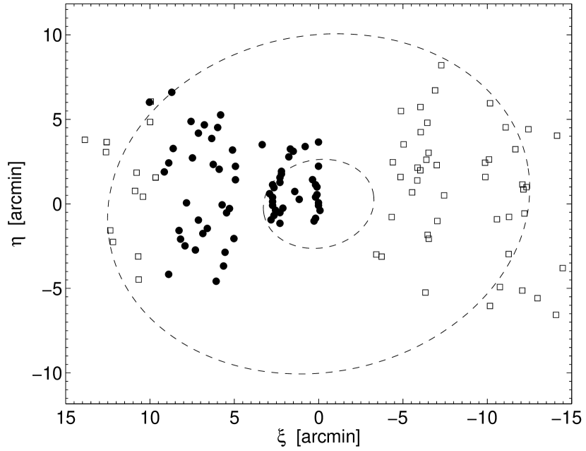
Figure 1: Location of our targets centered on the LeoI dSph at ($\alpha,\delta)=($10:08:28, +12:18:18). Red giants observed with GMOS are shown as filled circles, DEIMOS targets are depicted as open squares. Overlaid ellipses designate respectively Leo I’s core and nominal tidal radius at 3$\farcm$3, 12$\farcm$6, respectively. The system’s ellipticity and position angle are assumed to be 0.21 and 79$\arcdeg$.

One part of our observations was carried out in queue mode with the Gemini Multiobject Spectrograph GMOS at the 8-meter Gemini North telescope, Hawaii, over four nights between December 2004 and January 2005. These data were obtained under photometric conditions and a clear sky. The camera consists of three adjacent 2048$\times$4068 CCDs, which are separated by gaps with a width of $\sim$37 pixel each. We used 0$\farcs$5 wide multiobject slits and the R400+G5305 grating set in two modes, with central wavelengths of 8550 Å and 8600 Å, providing a spectral coverage of 1800 Å. This dithering enabled us to efficiently interpolate the spectra across the CCDs’ gaps during the later coaddition process. The CCDs were binned by 2$\times$4 during readout and the resulting spectra have a nominal resolution of 2200. In total, we targeted 68 red giants spread over three different fields in the eastern half of the galaxy (see Fig. 1, Table 1). Each of the three fields was exposed for three hours in total, where we split up the exposures into $3\times 1800$ s per setup (i.e., each of the two wavelength modes) to facilitate sky subtraction and cosmic ray removal. Due to bad weather, the central pointing (Field 3, see Table 1) was exposed for only 3600 s in total.

The other part of our data was obtained with the DEep Imaging Multi-Object Spectrograph (DEIMOS) at the 10-meter Keck II telescope. Leo I was observed on the DEIMOS multislit spectrograph on the Keck II telescope on February 6 to February 8, 2005. Conditions were mediocre, with high humidity and poor seeing, but approximately six hours of Leo I observations were obtained, consisting of five slit masks concentrated on the dSph’s periphery. We used the 1200 line/mm grating. The slits were $0.7^{\prime\prime}$ in size, and our resolution was about 0.3 Å per pixel.

2.3 Data Reduction

2.3.1 GMOS data

The GMOS data were reduced using the standard GMOS reduction package in IRAF, starting with the bias frames taken as part of the day-time calibration process. Spectroscopic flat-field exposures were obtained adjacent to each set of science exposures, from which we could model and remove the spectral signature and spatial profile of the illumination pattern. Through dividing by the remaining normalized flat-field frame, we ensured a complete removal of any residual sensitivity variation. Since the CuAr wavelength calibration frames were taken up to four days before and/or after the science spectra, during which time the telescope flexure may significantly change, we had to rely on the skylines of each individual science exposure to obtain an accurate wavelength solution. Hence, we chose a number of strong and isolated, unblended night-sky OH-emission lines around the CaT region from the atlas of Osterbrock et al. (1996, 1997). Fitting the respective lines with a low- order polynomial yielded a RMS uncertainty in the wavelength calibration of the order of 0.05 Å, corresponding to $\sim 2$ km s^-1 at our region of interest. A crucial step in the analysis of CaT absorption features consists of the accurate subtraction of the prominent skylines in the near-infrared spectral region. While the centers of the first two of the Ca triplet lines are unaffected by adjacent skylines at Leo I’s systemic velocity, the third Ca absorption line coincides with the dominant OH-band at $\sim$8670 Å. These undesired contaminants are efficiently removed by the software by fitting a low order polynomial to the background and subtracting this fit column by column from the science spectra. Moreover, the accuracy of our sky subtracted spectra (after coaddition) was improved by the fact that we obtained spectra with the slit centred both at the centre and offset towards the right and left hand side of the stellar seeing disk, yielding a better coverage of the average sky background. Finally, the extracted spectra were shifted towards the local standard of rest barycenter and median-combined using a standard $\sigma$-clipping algorithm. The average S/N ratio achieved throughout our reductions is $\sim$28, with a minimum of 5.3 at I = 19.6.

2.3.2 DEIMOS data

The DEIMOS data were reduced using the DEEP pipeline, developed by the DEEP2 project at the University of California-Berkeley and based on the IDL spectral reduction pipeline of the Sloan Digital Sky Survey (Abazajian et al. 2004). The DEEP pipeline first identifies spectra using tungsten lamp flatfield exposures, and then finds a two dimensional (pixel-by-pixel) wavelength solution for each spectrum, assisted by a DEIMOS-specific optical model. Typically, the solution is accurate to 0.005Å. All calibration images were taken at the start of each night; this is possible because the spectrograph optical system is stabilized using an active flexure compensation system. Sky subtraction is performed using a $b$-spline sky model. In the last stage, the sky-subtracted two-dimensional spectra are extracted into one-dimensional flux and variance spectra in the form of FITS tables. The variance spectrum is finally used to compute the spectral S/N ratio. The S/N achieved throughout our processing reaches $\sim$45 for the brighest targets and is as low as 5 for the faintest stars at I = 21.2.

Generally, the DEEP pipeline worked as expected. For certain exposures, however, the slit identification and tracing in the flats failed, and we found that the sensitivity parameter controlling slit detection had to be adjusted.

2.4 Radial Velocities

Radial velocities were derived from our final reduced set of spectra by cross-correlating the three strong Ca lines at $\lambda\lambda 8498,8542,8662$ against a synthetic template spectrum of the CaT region using IRAF’s cross-correlation package fxcor. The template was synthesized using representative equivalent widths of the CaT in red giants. The final velocity difference between object spectrum and the rest-frame template was then determined from a parabolic fit to the strongest correlation peak.

2.5 Velocity errors

The formal velocity errors returned from the cross-correlation in IRAF have a median value of 1.7 km s^-1. However, we have found in past studies that the fxcor estimates are generally too optimistic (see e.g., M98; Kleyna et al. 2002). Since we have only single epoch data at hand, lacking the possibility to compare the velocity stability over a longer time period, we cannot estimate the true uncertainties through the discrepancies of measurements taken at different times (Vogt el al. 1995, M98). For the GMOS data, we rather follow the prescription of Kleyna et al. (2002) and divide the data of the brightest stars (with $I\leq 19$ mag) into two final sets of spectra, the first comprising those individual spectra with a central wavelength of 8550 Å and the second being those centered at 8600 Å. Each of these sets was separately cross-correlated against the template. We use the discrepancy between the two resultant velocities as an estimate of the true measurement error. Hence, we rescaled the Tonry-Davis $R$-based errors (Tonry & Davis 1979) returned by fxcor to obtain the expected reduced $\chi^{2}$ discrepancy of unity. We found that we had to apply a scale factor of 2.7 to yield an accurate estimate of our velocity errors. In order to check whether our wavelength calibration, which is based on only a narrow spectral window around the CaT has introduced any bias, we also determined radial velocities by cross-correlating each of the three Ca lines separately against the same template. In this case, the mean deviation of the resultant velocities did not exceed 1.8 km s^-1. These uncertainties were added in quadrature to the formal measurement errors (including the above Tonry-Davis $R$ scaling) to yield the final velocity error, which we show in Table 2. The final GMOS data set contained 68 stars with a median velocity error of 5.0 km s^-1.

For the DEIMOS data, the nominal IRAF velocity errors were also rescaled by a common factor. The rescaling was performed by computing separate velocities for lines 1+2 and line 3 of the CaT, and then requiring the difference between the two velocities divided by the quadrature sum of the rescaled nominal errors to obey the expected $\chi^{2}$ statistics. The final DEIMOS member list includes 27 member velocities with per pixel $S/N>10$, and a median velocity error of 2.7 $\rm km\,s^{-1}$.

3 Radial Velocity Distributions

To determine an overall mean velocity and a global dispersion for Leo I, a prerequisite for an assessment of the targets’ membership, we used the maximization method described in Kleyna et al. (2002) and Walker et al. (2006a). In this approach, the probability that an observed distribution of velocities $v_{i}$ and corresponding measurement errors $\sigma_{i}$ is drawn from a Gaussian distribution with mean $\left<v\right>$ and dispersion $\sigma$ is given by

$$p\,(\{v_{i},\sigma_{i}\}|(\left<v\right>,\sigma)\,)\,\propto\,\\ \Pi_{i=1}^{N}\,\frac{1}{\sqrt{2\pi(\sigma^{2}\,+\,\sigma_{i}^{2})}}\,\exp\left\{-\frac{(v_{i}\,-\,\left<v\right>)^{2}}{2\,(\sigma^{2}\,+\,\sigma_{i}^{2})}\right\}$$ (1)

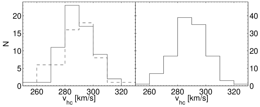
Figure 2: Radial velocity histograms of the GMOS data (solid line in the left panel), DEIMOS stars (dashed line, left panel) and combined GMOS plus DEIMOS set (right panel). All targets with velocities larger than 200 km s^-1 are shown. Within this range, two targets (at 251 and 324 km s^-1, respectively) fall outside a $\pm 3\sigma$-cut.

It is mathematically more convenient to calculate the natural logarithm of this expression, and maximizing $\ln p$ is equivalent to maximizing $p$ itself. Rejecting stars deviating more by than 3$\sigma$ as likely non-members, we iterated until convergence (requiring that the solution from subsequent iterations changed by no more than 0.005 km s^-1). The respective uncertainties in the mean and dispersion were then calculated from the covariance matrix (Walker et al. 2006a). This procedure yielded a mean systemic velocity of Leo I of (284.2$\pm$ 1.0) km s^-1 and a dispersion of 9.9 $\pm$1.5 km s^-1 from the combined GMOS plus DEIMOS sample, (284.6$\pm$1.5, 9.9$\pm$2.1) km s^-1 for the GMOS data alone and (283.8$\pm$1.5, 9.9$\pm$2.1) km s^-1 as derived from the DEIMOS targets only. The mean velocities and global dispersions are tabulated in Table 3 separately for the different fields and Fig. 2 shows the resulting histograms.

This compares to a value of $287.0\,\pm\,1.9$ km s^-1 as found by M98 and their respective dispersion of $8.8\,\pm 1.3$ km s^-1 for stars in the innermost $3\farcm 5$.

If we take the $3\sigma$-cut as a membership criterion, 5 of the 68 GMOS targets and 5 of the red giants from the DEIMOS sample have to be rejected as foreground contamination, where 4 out of these 5 stars in each sample have velocities below 200 km s^-1. In order to generate the final sample for determining the dispersion profile of Leo I we combined both of our GMOS and DEIMOS sets by shifting them to a common median velocity. This procedure is justified by the lack of any significant radial gradient in the velocities from DEIMOS, which is found to be ($-0.04\pm 0.18)$  km s^-1 arcmin^-1 so that such a shift does not introduce any artificial velocity gradient or a falsification of the dispersion profiles. At the end of this procedure, we found that our median velocity from the GMOS plus DEIMOS set differed from that of M98 by $-$2.8 $\rm km\,s^{-1}$, a difference significant only at the $p=0.31$ level (note that our sample has no stars in common with the M98 sample, which would allow for a direct comparison of the velocities). These values are finally listed in Table 2.

4 Kinematic tests for tidal damage and apparent rotation

Those dSph galaxies studied so far show no significant contribution from angular momentum to the systems’ dynamical structure: dSphs obtain their size and shape from anisotropic random pressure. This is, incidentally, an argument against an evolutionary transformation from dwarf irregular to dSph galaxies via ram pressure stripping (e.g., van den Bergh 1999; Grebel et al. 2003). More fundamentally, apparent rotation (generally visible in projection) is a characteristic signature of tidal disturbance. In this context, apparent rotation of the stellar component of a dSph is a test of possible tidal ‘heating’ of the stellar orbits in the course of the galaxy’s orbit within the external tidal field of the Milky Way. N-body simulations, e.g., of Oh et al. (1995) have shown that the velocity dispersion of a tidally-limited system is sustained at the actual virial equillibrium value. On the other hand, these simulations suggest that any strong dynamical effects on a dSph from the tidal field of the Galaxy can invoke streaming motions in the outskirts of the dwarf, which will lead to a systematic change in the mean velocity along its major axis, thus mimicking rotation (Piatek & Pryor 1995; Oh et al. 1995; Johnston et al. 1995; M98). A more detailed analysis of tidal effects on dSph galaxies is provided by Read et al. (2006b).

It has frequently been suggested in the literature that the detection of member stars well beyond the formal tidal-limit radius of dSphs, canonically defined via a single-component King model representation of the observed surface brightness profiles, is evidence for physical tides. A large number of dSphs have been claimed to show hints of extratidal stars and thus tidal disruption (Irwin & Hatzidimitriou 1995; Martínez-Delgado et al. 2001; Palma et al. 2003; Muñoz et al. 2005, 2006a, 2006b). Evidence for this has also been reported for Leo I (S06). What such studies show, in fact, is that the presumed parametric fit to the measured surface brightness (and/or direct star counts) is inappropriate at large radii. Given that there is no astrophysical basis to the application of a King model to a galaxy, an astrophysical interpretation of the corresponding labels as physical processes is fraught with peril. Evidence that a specific dSph is being affected by tides sufficiently strongly that its kinematics are affected can be provided most efficiently from a kinematic analysis. A test for apparent outer rotation is such a test.

With its present-day Galactocentric distance of (254$\pm$19) kpc and its high systemic velocity, Leo I is not expected to be affected by tides. M98 concluded from their kinematical data that the core of this galaxy has not been significantly heated by tides. S06 report on a large population of photometrical and radial velocity member red giant stars out to nearly two nominal tidal radii, which they interpret as evidence of tidal disruption. We note that also our sample comprises nine red giants outside $r_{tid}$, whose velocities suggest membership. We also emphasise that these statements tell us that the outer parts of Leo I are not well-fit by a single King model. Whether they tell us anything about the dynamics of Leo I remains questionable for the moment and has to await further dynamical tests.

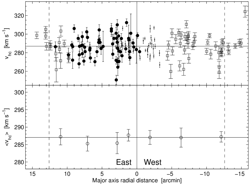
Figure 3: Distributions of individual radial velocities (top panel) and mean radial velocities (bottom panels) as a function of their major axis distance. The symbols in the upper panel are the same as in Fig. 1, while the small dots additionally depict the 33 data points from M98. The solid horizontal line indicates the global mean of our sample, while the dashed lines denote the formal King radius at 12$\farcm$6

In order to assess whether there is any significant indication of rotation in the Leo I velocities, which may help to elucidate the role of tides, we pursued two tests. First, we show in Fig. 3 the spatial distribution of our measured radial velocities (including M98’s 33 data points) along their projected major axis radial distance. In addition, we calculated the mean velocity as a function of radius, which is shown in the lower panel of Fig. 3. It is worth noticing that this mean velocity remains fairly constant across the range covered by our data and the deviations from the global mean of our sample are well within the errorbars. Moreover, we do not detect any significant sign of a velocity gradient in the inner regions as suggested by S06. If Leo I has been significantly affected by Galactic tides, one would expect an asymmetric excess of velocity outliers, with stars of higher or lower velocity typically lying on opposite sides of the galaxy due to the presence of possible leading and trailing tidal tails. In this vein, S06 report on the presence of a number of stars with higher velocities than the average in the outer regions to the western half of Leo I. The tidal model then predicts a comparable presence of low velocity stars towards the eastern extension. Although our sample contains one red giant at a large (western) distance with a radial velocity that is higher by $3.8\,\sigma$ than the sample mean, there is no apparent tendency of a systematically lower mean velocity of the targets at large distances towards the east.

While we find a mean radial velocity of 294.3$\pm$2.9 km s^-1 for the stars outside the formal tidal radius on the eastern side, the value for the stars towards the western half including (rejecting) the high velocity outlier amounts to 289.5$\pm$4.0 (285.7$\pm$5.5) km s^-1. From this point of view our data do not show any hint of significant rotation, nor an asymmetry of the velocities on either side along the galaxy’s major axis.

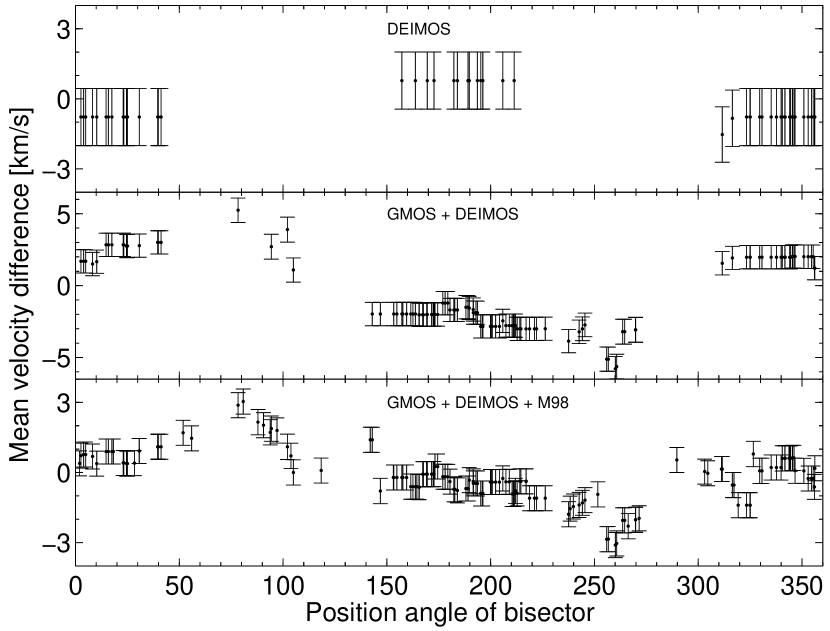
Figure 4: Tests for rotation in different subsamples of our data (as labelled): shown is the mean velocity difference with respect to rotation around axes at the respective position angles. A rotation signal around the major axis (at PA$\sim 79\arcdeg$) is distinguishable, but its significance is marginal. See text for a detailed discussion.

Secondly, we calculated the difference in mean velocity on either side of bisecting lines passing through each of the targets, assuming that each such line is a potential rotation axis. The axis yielding the maximum mean velocity difference is then taken as the “rotation axis”, with the associated velocity difference being an estimate of the amplitude of the rotation. Fig. 4 shows the resulting velocity differences for our dataset. Due to the confinement of our GMOS fields to the eastern half of Leo I, we cannot perform any test for rotation in this subsample alone. However, based on only the 56 candidate members from DEIMOS, we find a maximum velocity difference of 1.2 km s^-1. Nevertheless, the spatial distribution of these stars does not allow one to unambiguously determine a potential rotation axis (see top panel of Fig. 4). In the case of the combined GMOS and DEIMOS sample, the amplitude of the potential rotation reaches a value of 5.2 km s^-1 (middle panel of Fig. 4). When also the 33 stars from M98 are added, the mean velocity difference changes to 3.0 km s^-1 (bottom panel of Fig. 4). It is worth noticing that in both of the latter cases the axis of the maximum rotation signal occurs at a position angle (78$\arcdeg$, 80$\arcdeg$) which coincides with Leo I’s position angle of $(79\pm 3)\arcdeg$ (Irwin & Hatzidimitriou 1995).

In order to test the significance of these results, we constructed 10⁴ random samples of radial velocities at the observed spatial positions. The velocities were taken from a normal distribution with the same mean and standard deviation as in our observations, additionally allowing for a variation due to the measurement uncertainty. By means of this Monte Carlo simulation we find that the significance of the rotation in the DEIMOS sample is consistent with zero, whereas the amplitudes of the combined GMOS plus DEIMOS data sets and the full data including M98’s stars amount to a significance of 86.7% (1.5 $\sigma$) and 20% (0.3 $\sigma$), respectively. Thus the rotational signature we detected appears not to be statistically significant in either case. Consequently, we have no evidence of any kinematical effect due to Galactic tides operating on Leo I.

Another cause of apparent rotation is relative transverse motion. Unfortunately, there is no estimate of Leo I’s proper motion available in the literature at present. Hence, we cannot rule out the possibility that the amount of observed rotation is entirely due to the relative motion between the Sun and the dSph, $v_{rel}(l,b)$, in the Galactocentric rest frame. A non-rotating object will appear to rotate as seen in the heliocentric rest frame, provided there is a significant gradient in this relative motion across the dSph (see Walker et al. 2006a). We can attempt the inverse calculation: we tested whether one can constrain Leo I’s true proper motion by demanding that this galaxy does not rotate but the entire amplitude of the observed velocity gradient is caused by such projection effects. For this purpose, we calculated the Galactocentric rest frame velocity of each star through the formalism provided in Piatek et al. (2002) and Walker et al. (2006a). This was done for a wide grid of assumed proper motions, corresponding to transverse velocities from $-500$ to +500 km s^-1 in both $\mu_{l}$ and $\mu_{b}$. Regrettably, the full range of input ($\mu_{l},\,\mu_{b}$) was able to reproduce the observed apparent rotation amplitude adequately, so no deductions are possible. We then re-ran the same formalism by adopting a toy distance of 50 kpc to Leo I and secondly assumed its line-of-sight velocity as zero. In both cases the parameter space of possible proper motions increased even more. In consequence, we can neither unequivocally exclude the possibility that Leo I’s observed, though insignificant, velocity gradient is purely caused by the aforementioned projection effects or due to its large distance or systemic velocity, nor can we conclusively restrict its proper motion to a reasonable estimate.

5 Velocity Dispersion Profile

From their sample of 33 stars, M98 reported central velocity dispersions ranging from (8.6$\pm$1.2) km s^-1 to (9.2$\pm$1.6) km s^-1, which were obtained using several model-independent estimators. This is slightly lower than our global estimate from eq. 1, but consistent within the uncertainties.

We determined the velocity dispersion profile using the maximum likelihood method outlined in Kleyna et al. (2004). The data were binned such as to maintain a constant number of stars per bin, where we chose the binsize such that no fewer than ten stars were included. A Gaussian velocity distribution around the single mean velocity of the entire ensemble is then assumed for each radial bin, convolved with the observational errors. The member velocity distribution centred on the systemic velocity is then combined with an interloper distribution, $P_{int}(v)$, contributing a fraction $f_{int}$ to each bin. This allows the probability distribution of the true dispersion $\sigma$ in the bin through an extension of eq. 1:

$$p\,(\{v_{i},\sigma_{i}\}|(\left<v\right>,\sigma)\,)\, \propto \,\Pi_{i}\left[\,(1-f_{int})\,\frac{1}{\sqrt{2\pi(\sigma^{2}\,+\,\sigma_{i}^{2})}}\,\right.$$ (2)

$$\times \left.\,\exp\left\{-\frac{(v_{i}\,-\,\left<v\right>)^{2}}{2\,(\sigma^{2}\,+\,\sigma_{i}^{2})}\right\}+f_{int}P_{int}(v)\right]$$

We then perform a maximum likelihood fit over $\sigma$ and $f_{int}$, marginalise over the interloper fraction and finally find the most likely dispersion from the marginalised distribution.

We take account of the effects of the Galactic foreground interlopers in our data set by assuming various associated distributions $P_{int}(v)$ over the whole range of interest around the systemic velocity of Leo I. Consequently, we tested power-law velocity distributions with varying indices against the uniform case and against each other and found from a Kolmogorov-Smirnov (K-S) test that the resulting dispersion profiles were practically identical at a 100% confidence level. The velocity distribution of the ten non-member stars in our sample itself is best represented by a power-law with an exponent of $-0.7$ (with a K-S probability of 93%), whereas the K-S probability that these stars’ velocities are uniformly distributed is 52%. We emphasise, however, that the resulting dispersion profiles do not change with respect to the adopted parameterisation of the underlying interloper distribution. This is also to be expected, given the low total number of non-members sampled, a consequence of the overall high systemic velocity of Leo I relative to line-of-sight galactic halo stars. We will, for convenience, use the uniform case in the following. Typically, the peak interloper fraction for the outermost bin does not exceed 0.1 and is compatible with zero in the inner bins.

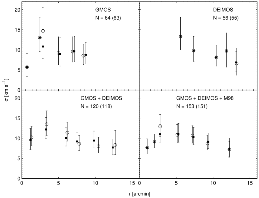
Figure 5: Velocity dispersion profile for different subsamples, as labelled, and rejection cuts. The numbers given refer to the sample size. Open circles refer to the full samples, whereas filled squares as well as the numbers in parentheses relate to the data cut at 3$\sigma$.

Finally, formal error bounds were determined by numerically integrating the total probability of the data set and finding the corresponding 68 per cent confidence intervals. Fig. 5 shows the resulting velocity dispersion profiles as a function of the projected spherical radius for different membership criteria, and separately for the subsamples.

5.1 Radial variations

Given the derived uncertainties in the profiles, the dispersion profile of LeoI can be considered to be approximately flat out to the nominal tidal radius for the majority of the data combinations shown. Exclusion of the 3$\sigma$-outlier in the last bin leads to only a marginal change. Inclusion of the data from M98 with our own data into the maximum sample decreases the dispersion in the central 3$\arcmin$ by $\sim$2 km s^-1, while the associated rebinning of the data introduces a small drop in the dispersion beyond 10$\arcmin$, quantifying the limited sensitivity of the binned dispersions to sample binning.

5.2 Absence or presence of kinematical substructure

Localized, kinematical structures in Local Group dSphs have been detected, specifically in the form of low velocity dispersion (cold) spatially clumpy substructure in the UMi dSph (Kleyna et al. 2003; Wilkinson et al. 2004). In Sextans a low velocity dispersion (cold) central core has been found (Kleyna et al. 2004) and independently the presence of an off-centered kinematically distinct subpopulation has been reported (Walker et al. 2006b). Such distinct cold features can be interpreted as the remains of dispersing star clusters, with their central locations arising due to the clusters being dragged towards the inner regions by dynamical friction (Kleyna et al. 2003, 2004; Goerdt et al. 2006). An alternative proposal involves the after effects of a merger between a dSph and an even smaller system (Coleman et al. 2004).

Despite the overall flatness of Leo I’s velocity dispersion towards larger radii, the profile does show some radial structure. A noteworthy radial feature is an apparent rise in the dispersion profile at $\sim 3\arcmin$ (r/r${}_{tid}\sim 0.25)$. This trend is persistent, regardless of radial binning and the chosen sample, and it is also inherent in the profile observed by Mateo (2005). The major difference between our profile and the one reported in Mateo (2005) is that his dispersion rises continuously out to 10$\farcm$5 after having reached its minimum after the bump. Hence, it cannot be excluded a priori that the local dispersion maximum may in fact be localized and physically real.

In order to test whether our data set supports the presence of any underlying localized kinematical substructure, we estimate the position-dependent dispersion using a non-parametric approach. We define the locally weighted, average dispersion as

$$\sigma\,(x,y)\,=\,\frac{\sum_{i=1}^{N}\left\{(v_{i}-\left<v\right>)^{2}-\sigma_{i}^{2}\right\}\,K(x,x_{i},y,y_{i},h)}{\sum_{i=1}^{N}\,K(x,x_{i},y,y_{i},h)}$$ (3)

(Walker et al. 2006b, after Nadaraya 1964; Watson 1964). Here, $v_{i}$ and $\sigma_{i}$ are as usual the observed radial velocities and associated uncertainties of the $N$ targets at the location ($x_{i},y_{i}$). The smoothing kernel $K$ is characterized by its smoothing bandwidth $h$, which we adopted as variable such as to include a fixed number $n$ of stars within 3$h$ at each location ($x,y$). For convenience in comparing our analyses, we follow the prescription of Walker et al. (2006b) in adopting a bivariate Gaussian kernel; hence
$K\propto\exp\left\{-\frac{1}{2}\frac{(x-x_{i})^{2}+(y-y_{i})^{2}}{h^{2}}\right\}$. The number of nearest neighbors $n$ was chosen sufficiently high to yield a statistically significant estimate of each local dispersion measurement, but sufficiently low so that any real spatial information would not be averaged out. Hence we varied $n$ from 5 to 30, corresponding to at most about 25% of the entire sample size.

The significance of any potential substructure in our data was then determined via detailed Monte Carlo modeling. For this purpose, 10³ random data sets were generated, where the ($x,y$) coordinates of our targets were preserved, but the observed velocities and error estimates were permuted with respect to their position. In this way, the sample mean and dispersion were retained, whereas any spatial information was dissolved. For each of these random data sets, the spatial dispersion distribution (eq. 3) and its maxima and minima were determined. The significance $p_{hot}$ ($p_{cold}$) of hot (cold) substructures at each spatial point was then defined by the fraction of random data sets with a maximum (minimum) dispersion, which is lower (higher) than the actual observed local dispersion $\sigma(x,y)$ (see Walker et al. 2006b).

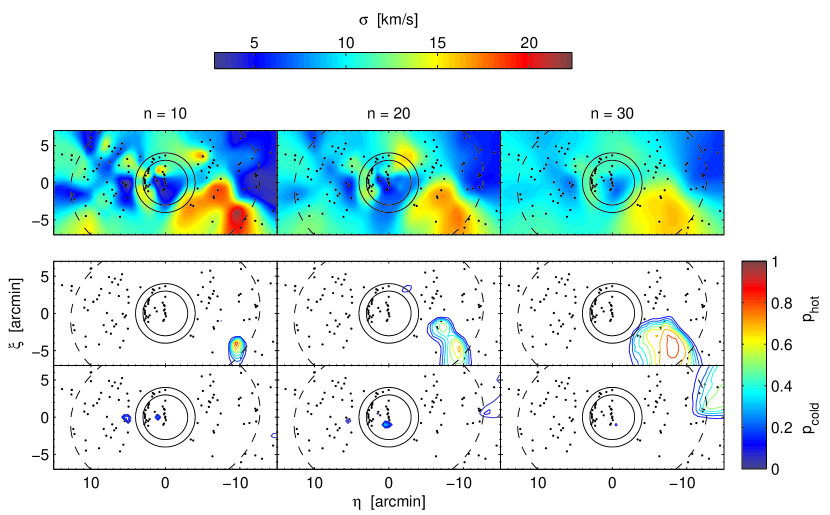
Figure 6: Top panel: Radial velocity dispersion estimator according to eq. (3), following the method of Walker et al. (2006b). Shown are the data for the combined GMOS + DEIMOS samples (small dots are the target locations), but the results do not alter after inclusion of the M98 sample. The middle and bottom panels display contours of the statistical significances $p_{hot}$ and $p_{cold}$ for the occurrence of any kinematically hot (middle) or cold (bottom) substructure. The individual panels show results for different choices of neighboring points included in the dispersion estimates. Contours are shown in intervals of 0.1. The dashed ellipse circumfers the nominal tidal radius and the two solid lines inscribe the interval of 3$\arcmin$–$4\arcmin$, in which the radial dispersion profile exhibits a bump. See text for details. [See the electronic edition of the Jounal for a color version of this figure.]

We do not find evidence of any localized cold substructure with low radial velocity dispersions in our data (see Fig. 6). In both the GMOS + DEIMOS data sets of Leo I and after inclusion of M98 targets, the significance of cold structures, $p_{cold}$, does not exceed 50% for any choice of the number of neighboring points. The typical value of this significance lies at 30%.

On the other hand, the presence of a physically real local maximum in the radial dispersion profile could indicate the presence of a locally hot structure at radii of $\sim$3–4$\arcmin$. Although the probabilities for an occurrence of hot substructure increase towards the nominal tidal radius, where the data are only sparsely distributed, the formal significances $p_{hot}$ are generally well below the 80% level. Hence, the apparent localized kinematical structure is consistent with statistical fluctuations about a constant dispersion value at the 1$\sigma$-level. In particular, there is no significant evidence of any localized structure at the radii in question – at loci between 3$\arcmin$ and 4$\arcmin$, the probability of an occurrence of any dynamically hot substructure is less than 15% for any reasonable choice of $n$.

Since the submission of our paper, S06 and Bosler et al. (2006) have presented kinematic data sets for Leo I. An analysis of the combined data sets (also including our data and those of M98), which yields a sample of the order of 400 red giants velocities, will aid the investigation of the the full kinematical structure of Leo I and is currently underway.

From our data, we conclude that the apparent rise in the velocity dispersion profile does not exclude the presence of any kinematical substructure, but it is probably not a localized feature.

5.3 (Non-) Influence of binaries

The presence of a significant population of binaries in any kinematical data set leads to an inflation of the observed velocity distribution, or, in other words, the true line of sight velocity dispersion of a stellar system is smaller than the observed dispersion, as soon as a non-zero binary fraction is considered. Moreover, the high-velocity tail of a binary distribution drives a distribution function away from Gaussian, so that an over-simple determination tends to produce larger errors in the derived velocity dispersion, which in turn may reduce the statistical significance of any real radial gradient in the dispersion profile (see error bars in Fig. 6). Fortunately, the effect of binary stars has been shown to be negligible in dSphs in the past. Hargreaves, Gilmore & Annan (1996) could effectively show by using Monte Carlo simulations that the velocity dispersion caused by pure binary orbits is small compared with the generally large observed dispersions in dSphs, provided that the ensemble of orbital parameters in the dSph stars is similar to the distribution in the solar neighbourhood. Likewise, Olszewski et al. (1996) concluded from their simulations that none of the kinematical estimates in the UMi and Draco dSphs significantly changes under the influence of binary stars. This finding was underscored by repeat observations of red giants in the Draco dSph (Kleyna et al 2002), and also Walker et al. (2006a) conclude from their repeat observation of red giant velocities in the Fornax dSph that the impact of binaries on the measured velocity dispersion is negligible. These observed kinematics did not show any evidence that would support an overall binary content larger than 40%. Moreover, the dynamically significant fraction in the Draco sample amounted to less than 5%. In the case of Leo I, Gallart et al. (1999a) argued from their modeled SFH based on deep HST color magnitude diagrams (CMDs) that it is unlikely that the total binary fraction in this galaxy exceeds 60%, again with a far lower dynamically significant number.

In order to explore the importance of binaries for the velocity dispersion profile of Leo I, we added an additional term to eq. 2, accounting for a binary star distribution $P_{b}(v)$, which is then convolved with the observed velocity distribution, in accordance with eq. 1 of Kleyna et al. (2002). The binary probability distribution $P_{b}(v)$ was adopted from Kleyna et al. (2002) and is based on the velocity measurements of Duquennoy & Mayor (1991) for a sample of solar-type primary stars in the solar neighbourhood. Kleyna et al. (2002) then obtained a realistic distribution by taking into account the giant branch binary evolution through circularization of the orbits.

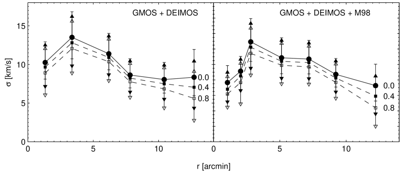
Figure 7: Radial velocity dispersion profiles for the subsamples as in Fig. 5. From top to bottom each curve was calculated with increased binary fractions $f_{b}$ (labelled right of the outer bins). The solid curve and filled points refer to the observed profile assuming no binaries. Solid (open) squares and dashed lines are drawn from a maximization assuming an $f_{b}$ of 0.4 and 0.8, respectively. In order to illustrate the effect of a binary population on the errors on the velocity dispersion, the respective error bounds of the profiles with $f_{b}>0$ are displayed as solid (open) triangles.

We note that the presence of a non-zero binary fraction does not alter the derived interloper fraction, which is still consistent with zero (less than 5% in the outermost bin). Fig. 7 shows velocity dispersion profiles obtained under the assumption of different binary fractions. The average errorbar on the velocity dispersion measurements increases by 10% for a binary fraction of 0.4 and by 25% for an implausibly large $f_{b}$ of 0.8. Likewise, the overall decrease of the dispersion profiles is, with less than 0.7 km s^-1 deviation for 40% binaries, well below the 0.5 $\sigma$ level. An increase of $f_{b}$ leads to a progressively more pronounced fall off of the underlying dispersion profiles. Nonetheless, the velocity dispersion profile assuming 40% binaries is consistent with that using no binaries at the 90% confidence level, as confirmed by a K-S test so that henceforth the effect of binaries on our observed line of sight velocity dispersion profiles is taken to be negligible.

6 Isotropic mass estimates

The simplest possible estimate of the mass profiles of dSphs uses single-component dynamical models, in which it is assumed that the mass distribution follows that of the visible component (“mass follows light”, e.g., Richstone & Tremaine 1986). In this context, King models (King 1966) were often used to describe both the surface density and the velocity dispersion profile. However, the parameters describing the visible content of dSphs, i.e., core radius $r_{c}$ and velocity dispersion profile $\sigma$, are in all cases studied in detail inconsistent with the mass-follows-light assumption inherent in this style of analysis (Kormendy & Freeman 2004). In the case here, where the approximately flat observed dispersion profile of Leo I suggests that the stars orbit in a (dark matter) halo which extends to radii larger than the nominal tidal radius of the observed light distribution, this historical approach is inappropriate. Where sufficient data exist, two parameter dynamical models for spherical stellar systems (Pryor & Kormendy 1990; Kleyna et al. 2002), additionally accounting for velocity anisotropies and a dark matter component or non-parametric modelling schemes (Wang et al. 2005, Walker et al. 2006a) are progressively being applied to reproduce observed profiles, in particular out to large radii.

Where only limited data exist, sufficient to define a binned dispersion profile but insufficient to support a full dynamical analysis of the distribution function, an intermediate level of analysis is appropriate, and is applied here. We pursued a simple approach to obtain an estimate of the galaxy’s mass and density profile by integrating Jeans’ equation (Binney & Tremaine 1998, eqs. 4-54 ff.) first under the assumptions of an isotropic velocity distribution and spherical symmetry, and below considering anisotropic distribution functions, using smooth functional fits to represent the light distribution and dispersion profile of Leo I.

In the case of an isotropic velocity distribution, the Jeans equations give rise to the simple mass estimator

$$M(r)\,=\,-\frac{r^{2}}{G\,\nu}\,\left(\frac{{\rm d}\,(\nu\overline{v_{r}^{2}})}{{\rm d}\,r}\right),$$ (4)

where $\nu$ and $\overline{v_{r}^{2}}$ denote the deprojected, three dimensional light density distribution and radial velocity dispersions, respectively. Both these quantities are obtained via direct deprojection of the observed surface brightness, $I(r)$, and projected dispersion profile $\sigma(r)$ adopting a convenient functional form, which in this case is a Plummer model (Wilkinson et al. 2006a, after Binney & Tremaine 1987). In this case, the surface brightness and associated, deprojected 3D profiles read

$$I(r)\, = \,\frac{I_{0}\,a^{4}}{(a^{2}\,+\,r^{2})^{2}},$$

$$\nu(r)\, = \,\frac{3\,I_{0}\,a^{4}}{4\,(a^{2}\,+\,r^{2})^{5/2}}.$$ (5)

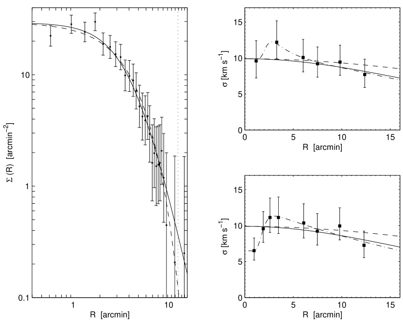
Figure 8: Left panel: Surface brightness profile of Leo I from Irwin & Hatzidimitriou (1995) together with the fit of a Plummer law (solid line) and an exponential fit (dashed). The upper right panel shows fits to the dispersion profiles from the GMOS plus DEIMOS sample, and the analog after inclusion of M98’s data is displayed in the lower right panel. Overplotted are fits of Plummer laws with different scale radii such as to reproduce a close-to flat (solid line) or falling (dashed) profile and also a modified profile, which incorporates the bump at $3\arcmin$ (dash-dotted).

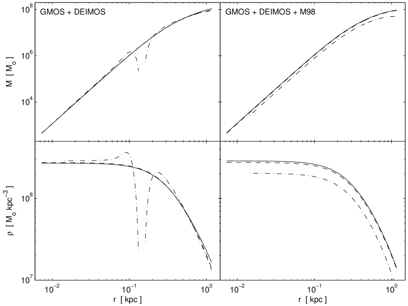
Figure 9: Mass (upper panel) and density (lower panel) estimates from Jeans equation, assuming an isotropic velocity distribution. The left panels each refer to the GMOS $+$ DEIMOS sample, whereas the right panels additionally account for the M98 data set. Different line types signify different approaches to fit the observed dispersion profile (see Fig. 8). The unphysical drop in the profiles of the left panels is due to the inclusion of an additional peak in the best-fit velocity dispersion profile, which exhibits a steep rising gradient in the inner regions opposed to a slower decline of the underlying Plummer profiles. These counteracting gradients are not as distinct after inclusion of the M98 sample so that the right panels do not display this drop.

The surface brightness profile of Leo I, which we adopted from Irwin & Hatzidimitriou (1995), is well fit by a Plummer model (left panel of Fig. 8) with a scale radius $a$ of $4\farcm 6$, which also nicely accounts for objects near the nominal tidal radius at $12\farcm 6$. Since the observed velocity dispersion profile, on the other hand, appears to be consistent with being flat, we fit this component with a Plummer profile with a large scale radius of 74$\arcmin$ to ensure a flat shape throughout the observed radius (right panels of Fig. 8). However, as Fig. 8 indicates, this argument is slightly sensitive to the value of the outer bin, which may give rise to a fall-off in the profile. Hence, we also chose a Plummer profile with a smaller radius (36$\arcmin$), which fits the observations best. In either case, the central value of the velocity dispersion $\sigma_{0}$ was determined as 9.8 km s^-1. These values hold only for the combined GMOS + DEIMOS sample. The inclusion of M98’s data leads to a decreased central velocity dispersion and consequently yields a lower central density $\rho_{0}$. The resulting density profiles in Fig. 9 fall off faster in the case that Leo I has a falling dispersion profile. Either density profile reaches a $r^{-1}$ slope at $\sim 3\arcmin$, but under the assumption of a flat velocity dispersion the density converges to the $r^{-2}$-law (linearly rising mass), whereas it tends to be consistent with a $r^{-2.5\dots-3}$ behavior towards the nominal tidal radius for the falling dispersion profile.

As discussed above our data suggest a rising feature in our velocity dispersion profile at approximately 3$\arcmin$. Although it has been shown above that this is not a statistically-significant localized structure, it may be physically real, and so provide useful constraints on the dark-matter mass distribution in Leo I. Consequently, we consider this particular shape by fitting the dispersion profile with an additional asymmetric Gaussian component of the form $\sigma_{bump}\,\propto\,10^{-\alpha\,r}\,\times\,\exp\,(-10^{(r-\mu)/p})$ overlaid on the Plummer profiles. The free parameters $\alpha$, $\mu$ and $p$ are then determined in a least-squares sense. Using this best-fit representation in the dynamical calculations results in an unphysical behaviour in the resulting mass profile, i.e., a drop in the cumulative mass and the density profile at the location of the bump (left panels of Fig. 9). This is attributed to a too steep rise in the additional component as opposed to the smooth decline towards larger radii. Hence, the associated gradient, which enters the Jeans’ equation, overwhelms the gradient of the declining portion in the dispersion and light profiles leading to a negative contribution in the derived mass profile. We note that varying the parameters of the Gaussian peak, retaining consistency with the GMOS + DEIMOS profile, does not remove this inconsistency. Conversely, a comparable fit to the GMOS + DEIMOS + M98 data does not exhibit this unphysical outcome, since for the respective best-fit profile the gradient in the innermost regions does not counteract the gradient of the more gradually declining profile at larger radii. We conclude that the failure of such a basic functional approach to simultaneously yield a physically expedient representation of all profiles considered suggests that we in fact do not see a real substructure. If, on the other hand, the dispersion profile could be modeled sufficiently well in either case and the radial feature was assumed to reflect a real structure, its particular shape would result in a close to uniform density profile at central radii. This would be indicative of a central core in Leo I. We will explore the plausibility of cored mass profiles in the next Section.

The upper and lower mass- and central density limits were finally derived by determining a profile that reproduced the observed velocity dispersion profile within the measurement uncertainties on either side. An estimate of Leo I’s mass thus yields $M_{tot}=(8\pm 2)\,\times\,10^{7}\,M_{\odot}$ enclosed within the King radius of 12$\farcm$6, corresponding to 0.9 kpc at the distance of Leo I. The exact values depend on the choice of the formal representation of the line-of-sight velocity dispersion profile and are detailed in Table 4. Similarly, the central density is found to be $\rho_{0}=(2.8\pm 0.8)\,\times\,10^{8}\,M_{\odot}\,$ kpc^-3, which is, in the light of the measurement uncertainties, consistent with the value of $(3.4\pm 0.9)\,\times\,10^{8}\,M_{\odot}\,$ kpc^-3 obtained by M98 from single-component King fitting. The available dynamical mass estimates for dSphs yield total masses out to the radial limits of the respective kinematic data in the range of 3–8$\,\times\,10^{7}\,M_{\odot}$ (e.g, Mateo 1998, Wilkinson et al. 2004; Kleyna et al. 2004; Chapman et al. 2005; Walker et al. 2006a; Wilkinson et al. 2006a). This places Leo I in the upper range of known LG dSph masses. Adopting a total luminosity of $L=(3.4\pm 1.1)\,\times\,10^{6}\,L_{\odot}$ (Irwin & Hatzidimitriou) we find an isotropic mass-to-light ratio of $(M/L)_{tot}=(24\pm 6)\,(M/L)_{\odot}$ (see Table 4). This value is three times larger than the central value quoted by M98, who obtained their estimate based on analyses of the galaxy’s core region and adopted a higher luminosity of $L=4.9\,\times\,10^{6}\,L_{\odot}$. If we adopt this latter value for $L$, we obtain a $(M/L)_{tot}$ of 17$\,(M/L)_{\odot}$. Moreover, S06 derive an estimate of 5.3 $(M/L)_{\odot}$, again with an underlying higher total luminosity of $7.6\,\times\,10^{6}\,L_{\odot}$, and based on core fitting and their value of the central velocity dispersion.

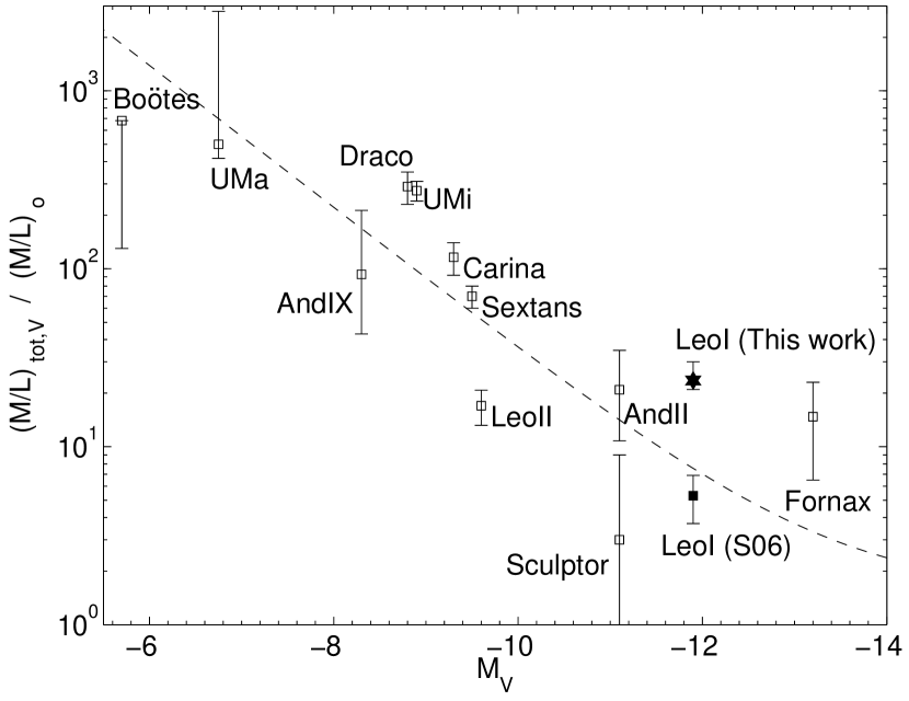
Figure 10: Mass-to-light ratios for LG dSphs (after Wilkinson et al. 2006a). The most recent individual mass estimates are from the sources cited in the text. The dashed line assumes a stellar (M/L)_V of 1.5 in solar units and a dark matter component of 3$\times 10^{7}$M_⊙. Also shown for Leo I is the recent estimate of S06, who yield a lower value than the present work.

In Fig. 10 we plot the V-band mass to light ratios versus V-band luminosities of the known Galactic dSphs, including some of the recently discovered systems, like Ursa Major (Willman et al. 2005) and Boötes (Belokurov et al. 2006a), plus two of the M 31 companions with published masses. In particular, we adopted mass estimates from Mateo (1998) for Leo II and Sculptor, whereas more recent measurements were used for the other satellites (Côté et al. 1999 for And II; Wilkinson et al. 2004 for UMi and Draco; Kleyna et al. 2006 for Ursa Major; Chapman et al. 2005 for And lX; Wang et al. 2005 for Fornax; Wilkinson et al. 2006a for Carina and Sextans, and Muñoz et al. 2006b for Boötes).

The idea that dSphs may be dominated by dark matter out to large radii raises the intriguing question whether all these dwarf galaxies could be enclosed in comparable dark matter halos of similar total mass, as first pointed out by Mateo et al. (1993). This feature would then argue in favor of an intimate relation between the dark matter halos of the dSph systems. Moreover, cosmological simulations suggest that it is possible that there is a minimum mass for a dark matter halo that contains stars (e.g., Read et al. 2006a and references therein). It is also an interesting question to ask whether all the dSphs have similar mass haloes, as this might tell us something about the properties of the dark matter. Under such an assumption, the halos can be represented by the the simple relation

$$(M/L)_{tot}=(M/L)_{\ast}+M_{DM}/L,$$ (6)

where $(M/L)_{\ast}$ is the intrinsic mass-to-light ratio of the stellar component in the galaxy, $M_{DM}$ denotes the mass of the dark matter halo and $L$ is the integrated luminosity in the V-band (M98; Wilkinson et al. 2006a). It is realistic to assume that the (M/L)-ratio of the the luminous component in dSphs is of the order of the mean value observed in low-concentration globular clusters, which are characterised by low values implying no dark matter (Pryor et al. 1989; Moore 1996; Dubath & Grillmair 1997; M98; Baumgardt et al. 2005). We do not correct the observed M/L-ratios for the (small) effects of stellar evolution, accounting for each individual dSph’s SFHs. Thus we set $(M/L)_{\ast}=1.5\,(M/L)_{\odot}$. As the best fit dashed line in Fig. 10 implies, the observed dSphs scatter around the expected relation for a population of luminous objects that are embedded in a dark halo with a common mass scale of the order of 3$\,\times\,10^{7}\,M_{\odot}$. Considering the generally large scatter in such a (M/L)-$M_{V}$-diagram, Leo I fits well into the global picture and apparently is governed by the same uniform dark halo properties. It is hence worth noticing that Fig. 10 demonstrates that the narrow range of dSph velocity dispersions of 6–10 km s^-1, combined with their rather similar physical length scales, can generally be interpreted in terms of a common mass scale so that this kinematical piece of information can reliably be used as a proxy for an overall underlying mass distribution (see also Wilkinson et al. 2006a).

7 Velocity anisotropy

The mass estimates derived above are based on the assumption of an isotropic velocity distribution, i.e., the velocity anisotropy parameter $\beta=1-{\left<v^{2}_{\theta}\right>}/{\left<v^{2}_{r}\right>}$ was assumed to be zero. However, most of the kinematic studies of dSphs have revealed that a non-negligible amount of anisotropy is required to account for the shapes of the galaxies, and the observed dispersion profiles (Łokas 2001, 2002; Kleyna et al. 2002; Wilkinson et al. 2004). Since the neglect of a non-zero anisotropy has the effect of under- or overestimating the dark halo mass, we also shall consider this problem by solving the Jeans equation

$$\frac{{\rm d}\,(\nu\overline{v^{2}_{r}})}{{\rm d}\,r}\,+\,2\beta\,\frac{\nu\overline{v_{r}^{2}}}{r}\,=\,-\nu\,\frac{{\rm d}\,\Phi}{{\rm d}\,r}$$ (7)

for a varying $\beta$. Here, $\nu$ and $\overline{v_{r}^{2}}$ denote again the 3-dimensional light and dispersion profiles, and $\Phi$ is the gravitational potential associated with the underlying mass distribution $M(r)$. The actual observable quantity, the line-of-sight velocity dispersion $\sigma$, is then obtained by direct integration along the line of sight, and under the constraints $\rho\,\overline{v_{r}^{2}}\rightarrow 0$ for $r\rightarrow\infty$ and $\beta=$ const. This gives rises to the one-dimensional expression

$$\sigma^{2}(R)\,=\,\frac{2G}{I(R)}\,\int_{R}^{\infty}\, {\rm d}x \,\nu(x)\,M(x)\,x^{2\beta-2}$$

$$\times\,\int_{R}^{x}\, {\rm d}y \,\left(1-\beta\,\frac{R^{2}}{y^{2}}\right)\,\frac{y^{-2\beta+1}}{\sqrt{y^{2}-R^{2}}}$$ (8)

(Binney & Mamon 1982; Łokas & Mamon 2003; Wilkinson et al. 2004). By adopting analytical prescriptions for the involved functions, one can then proceed to derive $\sigma$ numerically.

In concordance with the previous section, we chose to describe Leo I’s surface brightness profile $I(R)$ and the associated 3D-deprojection with a Plummer-profile using the best-fit parameters to the observations. We then use two different representations of the mass profile $M(r)$, which enters this formalism, spanning the range of plausible mass distributions.

7.1 NFW halo mass distribution

Based on high-resolution cosmological simulations, Navarro, Frenk & White (1995, hereinafter NFW) demonstrated that the density profiles of dark matter halos are well fit by a simple function with a single free parameter, the characteristic density. This solution has been applied to a wide range of halo masses, ranging from galaxy clusters to small scales such as the cosmological dark matter halos associated with the dSphs. Upon transformation of the variables, the density profile corresponds to a mass profile of the form

$$\frac{M(s)}{M_{v}}\,=\,g(c)\,\left\{\ln(1+cs)\,-\,\frac{cs}{1+cs}\right\},$$ (9)

where $s=r/r_{v}$ denotes the radial distance in units of the virial radius and $M_{v}$ is the mass enclosed within the virial radius. The latter is generally identified with the total mass of the halo. Finally, the concentration parameter $c$ is used to describe the shape of the profile and defines the amplitude function

$$g(c)\,=\,\left[\ln(1+c)\,-\,c/(1+c)\right]^{-1}.$$ (10)

For a detailed discussion of these parametrizations and the model, we refer the reader to NFW or Łokas & Mamon (2001). Since the NFW-profile has the unphysical disadvantage of diverging at large radii, it is convenient to consider only radii within a certain cut-off radius. We follow long-standing practice and assume this cut-off to coincide with $r_{v}$; beyond this point, the overall density distribution becomes unreliable in most natural cases (e.g., Łokas & Mamon 2001).

The concentration $c$ has been shown to scale with mass. Here we adopt an extrapolation of the formulae derived in the $N$-body simulations for $\Lambda$CDM cosmology of Jing & Suto (2000) to the small masses of dwarf galaxies. Hence,

$$c\,=\,10.23\left(\frac{h\,M_{v}}{10^{12}\,M_{\odot}}\right)^{-0.088},$$ (11)

where $h$ denotes the Hubble constant in units of 100 km s^-1 Mpc^-1. In concordance with current cosmological results, we will use $h$=0.7 for the remainder of this work. Likewise, the virial radius is related to the virial mass via

$$r_{v}\,=\,\quad 206\left(\frac{M_{v}}{10^{12}\,M_{\odot}}\right)^{1/3}\qquad\left[kpc\right]$$ (12)

This leaves $M_{v}$ and the anisotropy $\beta$ (assumed to be constant) as the only free parameters to be determined in a fit of the NFW model profile to the observations.

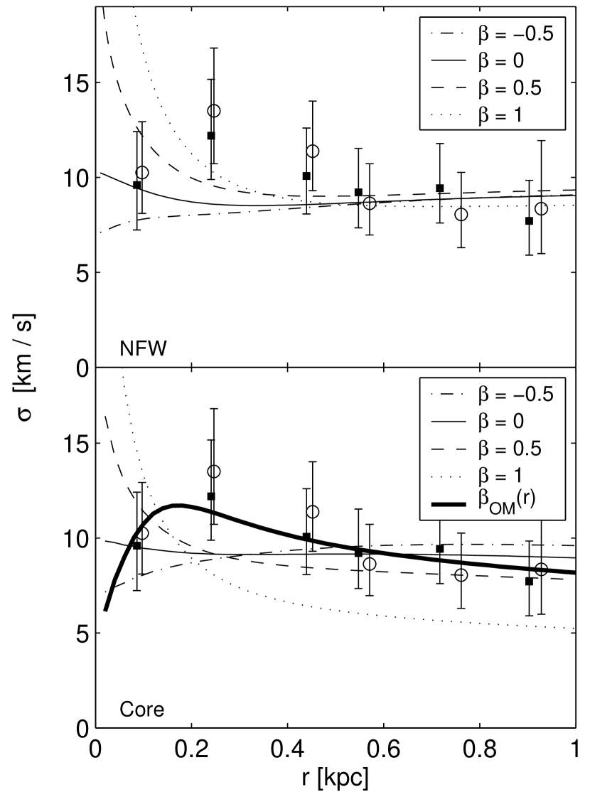
Figure 11: Predicted velocity dispersion profiles with varying degree of anisotropy ($\beta$) for two different halo density profiles, namely, cuspy (“NFW”, top panel) and a cored halo (bottom panel). The inner regions are consistent with isotropic orbits, whereas the outer regions do not rule out a certain amount of radial anisotropy. The lower panel also contains a curve for the case of a radial varying anisotropy parameter, $\beta_{\rm OM}$, after Osipkov (1979) and Merrit (1985), which represents our data reasonably well.

As Fig. 11 (top panel) implies, none of the values for the anisotropy which we have considered yields an adequate fit of the overall dispersion profile. It rather appears that a progressively radial anisotropy is needed to explain the observations at larger radii, whereas the inner parts of the velocity dispersion are best represented by an isotropic velocity tensor. It is worth noticing that the innermost bin, with a smaller value for the dispersion in the sample after inclusion of the M98 data points, may suggest the presence of some tangential anisotropy in the innermost regions. However, based on the observations, $\beta$ is unlikely to fall below $-0.5$. For the four different $\beta$ curves that we tested (i.e., $-$0.5, 0, 0.5 and 1), we obtained reduced $\chi^{2}$ values of (0.2, 0.16, 0.22, 0.78). The final best fit in terms of a minimized $\chi^{2}$ was achieved for $\beta$ = 0.05 so that the overall profiles are in agreement with an isotropic velocity distribution. The resultant best-fit total virial mass is $M_{v}$ = 1.0 $\times 10^{9}\,M_{\odot}$, with a corresponding virial radius of $r_{v}=21$ kpc and a concentration $c=19.4$. Furthermore, the mass within the nominal observed tidal radius amounts to 7.7$\times 10^{7}\,M_{\odot}$. It is, unsurprisingly given the near-isotropic distribution deduced, in good agreement with the value obtained under the assumption of a purely isotropic velocity distribution.

7.2 Cored halo profile

The density profile that we obtained under the assumption of velocity isotropy appears to be indicative of a flat, close to uniform density core at small radii (see bottom panels of Fig. 9). In conjunction with the observational indications of cored density profiles in low-luminosity galaxies and in particular in some of the dSphs (Łokas 2002; Kleyna et al. 2003; Strigari et al. 2006; Wilkinson et al. 2006a) this prompted us to also consider this particular density distribution in our calculations of Leo I’s dispersion profile (eq. 7). We parameterize the cored density profile in terms of a generalized Hernquist profile (Hernquist 1990; Zhao 1996; Read & Gilmore 2005) as

$$\rho(r)\,=\,C\,\left(\frac{r}{r_{s}}\right)^{-\gamma}\,\left[1+\left(\frac{r}{r_{s}}\right)^{\alpha}\,\right]^{(\gamma-3)/\alpha}$$ (13)

where $C$ is a normalization constant, $r_{s}$ is a scale radius, $\gamma$ is the log-slope of the density profile within $r_{s}$ and $\alpha$ determines the smoothness of the transition towards the density profile at larger radii. The case of $\alpha\equiv 1$ has often been discussed and fit to dispersion profiles in the literature, since it allows one to envisage a broad class of dark matter halo representations (Jing & Suto 2000; Łokas 2002). A slope of $\gamma>0$ then corresponds to the cuspy halos, where NFW-like profiles as discussed above are represented by $\gamma=1$. The opposing class of models with a cored halo is realized by $\gamma=0$.

It turns out that a least squares fit under the constraint $\alpha=1$, yields an unsatisfactory representation of our observations. Thus we chose to use the profile according to eq. 13 in our fits, leaving $C$, $r_{s}$, $\alpha$ and $\gamma$ as free parameters. The resulting parameters of $r_{s}=0.3$ kpc, $\alpha=1.6$ and $\gamma=0$ improved the reduced $\chi^{2}$ from 55 (3-parameter fit) to 13 (4 parameters). It is worth noticing that indeed the best fit was obtained for a pure core profile ($\gamma\equiv 0$). Fig. 11 (bottom panel) displays the resulting radial velocity dispersion profiles for varying degrees of (constant) anisotropy.

As for the case of the cuspy dark halo treated above, we find that our observed velocity dispersion is broadly consistent with an isotropic velocity distribution,where the best fit yielded a $\beta$ of 0.05. Still, the observations allow for a wider range in the anisotropy, from $-$0.5 to 0.5. In this context, a slight amount of tangential anisotropy can account for the shape of the profile toward the inner regions, whereas significant radial anisotropy is ruled out at all radii. The values for the associated reduced $\chi^{2}$ statistics for the cored halo are (0.39, 0.25, 0.40, 1.94) for respective $\beta$ values of ($-$0.5, 0, 0.5, 1).

Finally, we also adopted a radially varying anisotropy in our calculations, where we parameterized $\beta$ according to the traditional prescriptions by Osipkov (1979) and Merrit (1985) as $\beta_{\rm OM}(r)\,=\,{r^{2}}/({r^{2}+r_{a}^{2}})$, where $r_{a}$ denotes the anisotropy radius, at which the transition from isotropic to radial orbits occurs (see also Łokas 2002). Under the assumption of a cored density profile and this particular $\beta(r)$, we can fit our observed line-of-sight velocity dispersion profile fairly well (see the thick solid line in Fig. 11, bottom panel). The best-fit (at a $\chi^{2}$ of 0.02) is then obtained for an anisotropy radius of $r_{a}=0.13$ kpc. In particular, the resulting curve is able to account for the observed rising shape of the profile discussed in Sect. 5.2, albeit by requiring a considerable amount of radial anisotropy at relatively small radii.

Another possible explanation of the dispersion profile of Leo I might be the presence of two stellar components with different length-scales and associated different velocity dispersions. McConnachie et al. (2006) have recently presented dispersion profiles derived for such a system. Their profiles bear a striking resemblance to that of Leo I and might account for the initial rise in the projected dispersion.

In concluding we note that the enclosed mass within the tidal radius amounts to 8.5$\times 10^{7}\,M_{\odot}$ under the assumption of a cored halo in Leo I. This value is larger than under the assumption of a NFW-like mass distribution, but still in agreement with the numbers derived from the Jeans equations above.

8 The Metallicity of Leo I

The observed wavelength region in the near-infrared and our spectral resolution, coupled with the S/N of our observations also enabled us to get an estimate of the red giants’ metallicites from the equivalent widths (EWs) of the Ca triplet (CaT). This procedure succeeded for 58 of the radial velocity member stars targeted with GMOS, all of which lie well within the nominal tidal radius. For the remainder of our targets, the S/N did not allow us to reliably measure EWs, where a lower limit for these measurements was S/N$\sim 10$.

8.1 Calibration of the metallicity scale

The prominent Ca II feature may be calibrated onto global metallicities since the linestrength is a linear function of metallicity for red giants. By defining a reduced width $W^{\prime}$, which accounts for the luminosity difference between the targeted star and the horizontal branch (HB) of the system, one can effectively remove any dependence on stellar gravity, effective temperature, and distance. Thus, the CaT has become a well defined calibrator for assessing the metallicity for old, globular cluster-like populations (Armandroff & DaCosta 1990, Rutledge et al. 1997a,b). Consequently, the derived line widths are generally calibrated onto reference scales for globular clusters of known metallicities (Zinn & West 1984; Carretta & Gratton 1997; Kraft & Ivans 2003). Leo I has a prominent old population (e.g., Held et al. 2000), but its dominant populations are of intermediate age (e.g., Gallart et al. 1999a,b). Nonetheless, we can still apply the CaT technique, since Cole et al. (2004) have extended its calibration to younger ages. These authors demonstrated that the CaT technique can be used within an age range from 2.5 to 13 Gyr and for a metallicity range spanning $-2<$ [Fe/H] $<-0.2$. Since our Leo I observations aimed primarily at measuring accurate radial velocities, we did not target any globular clusters, which could have been used as calibration standards for the CaT technique. Hence, we had to rely on standard calibrations devised in the literature. Following long standing practice, we employed the definition of Rutledge et al. (1997a, hereafter R97a) for the linestrength of the CaT as the weighted sum of the EWs, giving lower weight to the weaker lines:

$$\Sigma W\,=\,0.5\,W_{8498}\,+\,W_{8542}\,+\,0.6\,W_{8662}.$$ (14)

For a few of the spectra the Ca line at 8498Å was too weak to be accurately measured or was hampered by too low a S/N over the respective bandpass. In this case we used a relation derived from the high S/N spectral measurements of a sample of Galactic globular clusters from Koch et al. (2006a):

$$\Sigma W\,=\,1.13\,(W_{8542}\,+\,0.6\,W_{8662})\,+\,0.04.$$ (15)

This relation was applied to the low-quality spectra where only the two strongest lines had S/N$>$10. R97a defined the reduced width as

$$W^{\prime} = \Sigma W+0.64\,(\pm 0.02)\,(V-V_{HB})\,,$$

where $\Sigma W$ denotes the CaT linestrength and V_HB is the magnitude of the horizontal branch of Leo I. For Leo I, the HB luminosity is (22.60 $\pm$ 0.12) mag according Held et al. (2001), who measured it based on this galaxy’s RR Lyrae population.

The final calibration of the reduced width in terms of stellar metallicity is then obtained via the linear relation

$$\left[Fe/H\right]_{CG} = -2.66\,(\pm 0.08)+0.42\,(\pm 0.02)W^{\prime}\,$$

(Rutledge et al. 1997b), where we chose to tie our observations to the reference scale of Carretta & Gratton 1997, hereafter CG97) unless stated otherwise.

The EWs of the calcium lines were determined in analogy to the methods described in Koch et al. (2006a), i.e., by fitting a Gaussian plus a Lorentzian profile across the bandpasses defined in Armandroff & Zinn (1990) and summing up the flux in the theoretical profile. The median formal measurement uncertainty achieved in this way, incorporating EW measurement and calibration errors, is 0.12 dex. However, we note that the intrinsic accuracy of the CaT based metallicity measurements may be significantly lower. For instance, variations in the HB level of a composite stellar system with both age and metallicity can give rise to a systematic error of the order of 0.05–0.1 dex (Cole et al. 2004). Moreover, the general incompatibilitiy between the [Ca/Fe] ratio in dSphs and the Galactic globular clusters adopted as calibrators is another source of uncertainty. High resolution abundance studies of red giants in dSphs have shown that their $\alpha$-element abundance ratios lie significantly below those in Galactic halo stars at comparable metallicities (e.g., Venn et al. 2004), and also the two red giants observed in Leo I by Shetrone et al. (2003) follow this trend of $\alpha$-deficiency. Moreover, the low-resolution studies of Bosler et al. (2006) underscore these low abundance ratios as compared to the halo. The systematic uncertainties resulting from such a priori unknown variations in [Ca/Fe] for our targets can reach up to 0.2 dex (e.g., Koch et al. 2006a). It is worth noticing that such effects can be overcome in future studies by calibrating the reduced width directly onto [Ca/H] (Bosler et al. 2006), thus circumventing any dependence of the calibrations of the galaxy’s SFH, in contrast to the presently employed method.

8.2 Metallicity distribution

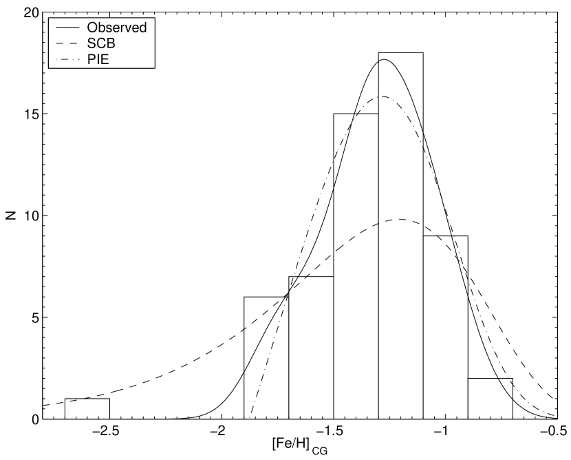
Figure 12: Metallicity distribution for the 58 GMOS radial velocity member stars, for which EWs could be measured. These were convolved by observational uncertainties to yield the solid curve. Overplotted are a modified simple closed-box model (SCB, dashed line) and a model using Prompt Initial Enrichment (PIE, dash-dotted line), scaled to the same number of stars.

Fig. 12 shows the resulting histogram of our metallicity estimates. The MDF is clearly peaked at a median metallicity of $-1.31\pm 0.02$ dex on the scale of CG97, with a measurement error of 0.12 dex ($-1.61$ on the scale of Zinn & West 1984; hereafter ZW84). This value is in excellent agreement with the study of Bosler et al. (2006), who derived a CaT metallicitity of $-1.34\pm 0.02$ dex (mean measurement error of 0.10) for a sample of 101 red giants (note, however that the lack of any common targets between the studies of Bosler et al. [2006] and ours does not allow us to compare measurements of individual stars). Our results also agree within the uncertainties with the low-resolution studies of Suntzeff et al. (1986), who obtained $-1.9\pm 0.2$ dex (ZW84). Moreover they are consistent with the estimates from photometric analyses, which broadly agree on a mean metallicity around $-1.6\pm 0.4$ dex (ZW84 scale; Demers et al. 1994; Bellazzini et al. 2004)

The formal 1 $\sigma$-width of the MDF is 0.25 dex. Taking into account a broadening due to the observational uncertainties, the intrinsic metallicity dispersion amounts to 0.22 dex. With a full range in [Fe/H]_CG97 of approximately one dex between $-$1.8 and $-0.8$ dex (note the most metal poor star, which we discuss below) we observe a smaller spread than is seen in a number of other dSphs (Shetrone, Côté, & Sargent 2001; Pont et al. 2004; Tolstoy et al. 2004; Koch et al. 2006a), where the MDF may span more than 2 dex and exhibits a well populated metal poor tail. Leo I has been shown to exhibit a rather narrow RGB. By means of detailed modeling of Leo I’s CMD and in particular of this narrow feature, Gallart et al. (1999a) suggested that this might be indicative of the absence of any significant chemical enrichment in this dSph. Clearly, the spectroscopic data show that this is not correct and that Leo I underwent considerable enrichment of at least 1 dex in total range.

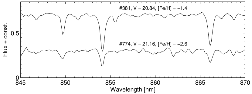
Figure 13: Spectra of the most metal poor star in our sample and a typical spectrum of a target around the peak metallicity. Apart from the three dominant Ca lines there are a few weak neutral metal lines detectable, which are not distinguishable from the continuum in the metal poorer target.

There is one object in the sample, #774, for which we derived a CaT based metallicity of $-2.61$ dex. There is no evidence in the spectrum that the linestrength of this target has been underestimated, since its S/N of $\sim$45 allowed an accurate determination of the triplet’s EWs (see Fig. 13). Although weak neutral metal lines around the CaT region do not show up clearly at our nominal spectral resolution and are thus mostly blended, there are still some additional absorption features discernible from the noise (see Fig. 13). Among these are for instance the distinct Fe I blend at $\sim$8514Å and a visible Fe I-line at $\sim$8689Å. Though clearly present in our stars with highest metallicities, these features are hardly detectable in the continuum of the metal poor candidate. By assuming appropriate line bandpasses around these two iron features, we employed the same fitting technique as for the CaT described in Section 8.1 in order to derive a rough qualitative estimate of these lines’ EWs in each of the stars, where possible. From this point of view, #774 is well consistent with being a rather metal poor object, in which these two EWs are practically governed by the continuum noise. Furthermore, its location well within the galactic boundary (2.5 core radii, 0.67 tidal radii, resp.), its consistency with the systemic velocity (99.9% confidence level) and the low interloper fraction around Leo I’s radial velocity make it appear unlikely that this star is a contaminating foreground dwarf.

8.3 Radial gradients and implications for evolutionary models

In those dSphs of the Local Group, in which both old and intermediate-age stellar populations have been detected, the younger components often are more strongly centrally concentrated. In a number of dSphs with predominantly old populations, population gradients have been found in the sense that red HB stars are more centrally concentrated than blue HB stars (e.g., Da Costa et al. 1996; Hurley-Keller et al. 1999; Harbeck et al. 2001; Tolstoy et al. 2004), a trend that is mirrored also by the presumably more metal-rich red giants. However, as also pointed out by Harbeck et al. (2001), this trend is not seen in all dSphs.

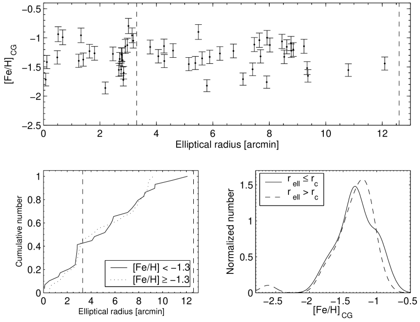
Figure 14: CaT metallicities of our radial velocity members vs. their elliptical radius (top). Nominal core and tidal radius are also denoted by vertical lines. The bottom left shows the cumulative number distribution versus radius of the metal richer component (solid line) and the metal poorer population (dotted line). These are practically indistinguishable. MDFs at different radii are displayed in the bottom right panel. These density distributions were convolved by individual measurement errors. No apparent trend of [Fe/H] with radius is discerned.

Since Leo I hosts dominant intermediate-age populations as well as old populations, one may expect that the more metal-rich and presumably younger stars should then also be more concentrated with respect to a spatially extended metal-poor population. Our data suggest, however, that the metal-rich and metal-poor components in our MDF are drawn from the same spatial distribution. This is reflected by the comparison of the cumulative radial distributions of the more metal-poor ([FeH] $<1.3$ dex) versus the metal-rich ([FeH] $\geq 1.3$ dex) populations in Fig. 14. Via a K-S test we could underscore this lack of a radial metallicity gradient at the 93% confidence level. This finding is in concordance with the lack of a considerable population gradient in Leo I’s CMD. As was reported by Held et al. (2000), both the old HB population and its numerous intermediate-age counterpart exhibit essentially the same spatial distribution (see also the right bottom panel of Fig. 14). In this respect, Leo I differs from other dSphs with prominent intermediate-age populations such as Carina (e.g., Harbeck et al. 2001; Koch et al. 2006a), Fornax (Grebel 1997; Stetson et al. 1998) and Leo II (Bellazzini et al. 2005). Moreover, we find that the kinematics of the metal poor and the more metal rich samples do not differ significantly, neither. This is also in contrast to what is found for different stellar components in many other dSphs (Tolstoy et al. 2004; Ibata et al. 2006): While the sample with [Fe/H]$<-1.3$ exhibits a dispersion of 9.1$\pm$2.8 km s^-1, for those stars with [Fe/H]$\geq-1.3$, $\sigma=10.7\pm$3.1 km s^-1, which is an insignificant difference in the light of the uncertainties.

This behavior may indicate that Leo I’s star formation occurred from a well mixed reservoir of gas that was little affected by local accretion of material or spatially localized outflows. In this vein, it was suggested by Held et al. (2000) that the size of this galaxy has not significantly changed and that it is unlikely to have undergone severe structural changes in the course of its evolution, i.e., since the first onset of star formation. In such a model one must assume that external effects such as tides, accretion or minor mergers may not have played a significant role in Leo I’s history, neither kinematically nor chemically. On the other hand, S06 claim that the preferential periods of SF in Leo I may be linked to perigalactic passages, which argues in favor of tidal interactions. Still, without extant detailed knowledge of this dSph’s orbit (via proper motions), this has to await further investigation.

8.4 Comparison with simple chemical evolution models

Present-day chemical evolutionary models agree on the fact that dSphs are mainly controlled by low SF efficiencies compared to the solar neighborhood, and by strong galactic winds of the order ten times the SF rate (Lanfranchi & Matteucci 2004). For want of a detailed model prediction of Leo I’s MDF from its SFH we follow long standing practice in applying basic models of chemical evolution to describe the observations (e.g., Pagel 1997, ch. 8), without employing any deeper nucleosynthetic or physical prescriptions. Such more detailed modeling is left for future work.

In that spirit, Fig. 12 shows the predicted MDFs for two simple models of chemical evolution. To start with, we obtained a best-fit representation of a modified simple closed-box model allowing for outflows, which is exclusively parameterized by the effective yield $p_{\mathrm{eff}}$. Basically, this value is proportional to the true nucleosynthetic yield and takes into account effects of the loss of metals. Consequently, the mean metallicity is reduced to below the true yield by the same factor, which relates the outflows and the actual SF rate. A low yield of 0.06 $Z_{\odot}$ is well able to reproduce the metal poor mean location of the peak of the MDF, when compared to the solar neighborhood, which peaks at around $-0.2$ dex (Nordström et al. 2004 and references therein). However, this prediction tends to overestimate the number of stars below $-1.8$ dex (note that the most metal poor object in our sample was excluded from the fit), leading to the well-known G-dwarf problem. We note that a comparison of these models, which are based on predictions for long-lived stars, to our observations of K-giants with predominantly negligible lifetimes is still valid, since the simple model of chemical evolution does qualitatively predict an excess of metal poor K-giants under the assumptions of a standard IMF and loss of metals from the galaxy (Koch et al. 2006b). Moreover, it has been shown that there is no noticeable difference between the K-giant MDF in the solar neighbourhood (McWilliam 1990) and the local G-dwarf MDF from, e.g., Nordström et al. (2004). Hence we carry on with the long-standing practice of applying the G-dwarf predictions to K-giant MDFs as tracers of low-mass stars.

After allowing for an admixture of a non-zero initial metallicity (prompt initial enrichment, PIE), the overprediction toward the metal poor tail is reduced and it turns out that a pre-enrichment of $Z_{0}\,=\,0.013\,Z_{\odot}$ yields a remarkably good representation of the overall shape of the observed MDF. We refer the interested reader to Koch et al. (2006a, 2006b) for a discussion of these standard models.

9 Summary and Conclusions

We have obtained radial velocity measurements for 120 red giants in the Leo I dSph. These data not only increase existing published samples by more than a factor of three, but also extend in radial distance beyond previous studies of the central regions of the galaxy (M98).

Although the weak velocity gradient that our data exhibit coincides with an apparent rotation about the observed major axis of Leo I, the associated amplitude has been shown to be insignificant. Moreover, we do not detect any trend of mean radial velocity with major axis distance, and in particular we do not find any evidence of an asymmetric velocity distribution towards the outer regions, in the sense that the eastern (western) halves of the galaxy would preferentially exhibit an excess of low (high) velocity outliers outside the formal tidal boundary. Supplemented by Leo I’s high radial velocity, which we confirmed, and its large distance from the Milky Way, Leo I most likely represents an isolated system, which is currently not affected by Galactic tides, at least from a kinematical point of view. This is also consistent with our detection of nine radial velocity members outside the nominal ‘tidal’ radius, and implies that the difficulty of the King-model functional fit to surface brightness data at some (outer) radius is not necessarily a dynamical evidence of a physical effect. ‘Tidal’ radii for dSphs, as typically derived from photometry, are labels, and are not proven to be related in any way to gravitational tides. The results of S06 indicate that Leo I’s surface brightness profile exhibits multiple breaks at large radii, where it deviates from common King models, while further recent photometric analyses do not provide any such clear evidence of photometric complexity above the noise level (Smolčić et al. 2006). Still the detection of dSphs’ stellar populations far out beyond the limiting radius, as in the case of Carina (Muñoz et al. 2006a), suggests that some dSphs may in fact be perturbed systems, at least in their outermost regions. Clearly this has implications for estimates of the dark matter content of dSphs at the largest radii, as tidal effects may inflate the projected dispersion in these regions.

Our derived projected radial velocity dispersion profile is flat out to the nominal tidal radius, a result which is turning out to be a very common feature among the dSphs of the MW system, being established in numerous studies of large radial velocity samples out to and even beyond their nominal tidal radii (Mateo 1997; Kleyna et al. 2001, 2003, 2004; Łokas 2001, 2002; Wilkinson et al. 2004; 2006a,b; Muñoz et al. 2005; Walker et al. 2006a; Westfall et al. 2006). Coupled with the overall high (M/L) ratios, and lack of unambiguous evidence for non-equilibrium effects, the prime explanation of flat dispersion profiles is that dSphs are dark matter supported at all radii, although the N-body simulations of S06 indicate that also tides could reproduce such features in Leo I.

Nevertheless, at its large present Galactocentric distance, tidal influences would be plausible only if Leo I’s orbit were close to radial. However, our current data set does not allow us to constrain its proper motions and any information about its orbit will have to await future accurate proper motion measurements.

It turns out that the observed dispersion profiles are largely consistent with an isotropic velocity distribution, but non-negligible amounts of radial (tangential) anisotropy may be needed to account for the shape of the dispersion profile at the largest (smallest) distances.

An apparent rise in the velocity dispersion profile at nearly the core radius was demonstrated not to be a localized dynamical substructure in the galaxy. By using simple prescriptions to describe the shape of the observed velocity dispersion profile we obtain an estimate of the enclosed mass within the nominal ‘tidal’ radius of 900 pc of $\sim$8$\times 10^{7}M_{\odot}$ under the assumption of velocity isotropy. Such a mass and the resultant high mass-to-light ratio of $\sim$24 ($M/L$)_⊙ are higher than previously derived values (M98; S06). From their ($M/L$) of $\sim$6–13 ($M/L$)_⊙, M98 concluded that Leo I contains a significant dark component. These estimates are in reassuringly good agreement with the values derived from light profiles obtained from high-quality photometric data under the assumption of an extended constant dark matter halo density (Smolčić et al. 2006). Hence, our results strengthen this view and are in concordance with an extended dark matter distribution with a halo mass of a typical scale ($\sim$3$\times 10^{7}M_{\odot}$), which is shared by the other dSphs of the LG.

By adopting a NFW density profile for Leo I, we estimate its total virial mass within its dark matter halo to be $\sim$1 $\times 10^{9}M_{\odot}$. The mass within the tidal radius is estimated to be $\sim$7.7 $\times 10^{7}M_{\odot}$. This does not change much under the assumption of a constant density core in Leo I, where the enclosed mass and best-fit anisotropy are consistent with the values from a cusped profile. Although the density profile obtained using Jeans equations, under the assumption of velocity isotropy, indicates a flat central core, this scenario is not significantly preferred against the NFW case if one exclusively argues on the base of the velocity dispersion profile. In general, the shape of the observations seems to indicate that dark matter in fact dominates this dSph at large and small distances. We are aware that analysis only of a dispersion profile $\sigma(r)$ is not sufficient to derive a unique kinematical distribution function of a stellar system. Unless more numerous data sets and in particular the higher moments of the velocity distribution are considered, there remains a degeneracy between anisotropy and density, leading to identical line-of-sight dispersion profiles (e.g., Merrifield & Kent 1990; Łokas & Mamon 2003). While in general such an analysis requires more data than is currently available for Leo I, this will be pursued in future papers dealing with more detailed dynamical modeling (Wilkinson et al., in preparation).

We derived metallicites for 58 of the member stars from the well established CaT calibration. In compliance with previous estimates that were drawn from both photometric and low-number spectroscopic analyses we find a mildly metal poor mean of $-1.31$ dex (CG97 scale) and a full spread in metallicity covering 1 dex. This is noticeably smaller than the ranges found in dSphs with extended or complex SFHs (Grebel 1997; Pont et al. 2004; Tolstoy et al. 2004; Koch et al. 2006a). This spread exceeds the predictions from CMD modeling if one accounts for the narrow RGB and Leo I’s existing intermediate-age population. Hence, there may be also a large range in ages present in Leo I, as hinted at by the presence of also an old population (Held et al. 2000, 2001) and the preliminary age determinations by Bosler et al. (2004). Practically all dSphs that contain significant intermediate-age populations do show a central concentration of their young components (Stetson et al. 1998; Harbeck et al. 2001; Bellazzini et al. 2005). Intriguingly, Leo I’s prominently younger and presumably metal rich population does not exhibit this distinct population gradient. Neither its stellar populations (Held et al. 2000) nor the metallicities we derived here show any evidence of radial gradients. In this respect, Leo I is rather unusual among these systems. This property may again point to a negligible role of external influences, such as localized accretion of material, in Leo I’s evolution, allowing for good mixing of its gas. Since tides would affect this mixing, it is therefore possible that its current large distance from the MW may be representative of its whole evolution and that it never approached the Galaxy very closely. This view is consistent with the finding that the fraction of intermediate-age populations is closely related to the dSphs’ Galactocentric distance (e.g., Grebel 2003 and references therein). This behavior can be taken as indicative of an increased influence of (e.g., ram pressure) stripping close to the MW (van den Bergh 1994; Grebel 1997; Grebel et al. 2003) and will not have affected Leo I to a major extent. We note, however, that S06 argue that the presence of the various stellar populations in Leo I may in fact be linked to much closer perigalactic passages, which facilitated the onset of SF, a scenario that would then incorporate a non-negligible role of tides in Leo’s evolution.

We identified one comparatively metal poor star in our sample, which is unlikely to be a foreground contaminant. With its likely [Fe/H] of $\sim$$-$2.6 (CG97 scale) it lies 0.8 dex below the metal poor tail of our observed MDF. It has been suggested that the explosion of only one massive pregalactic Population III star produces a sufficient amount of energy to expel the entire gas from the first (high-$z$) cosmological minihalos (Bromm et al. 2003). If the expelled gas falls back afterwards, the subsequently forming generation of stars, which we would observe as the most metal poor and the oldest stars in dSphs, should bear the chemical signature of these Population III stars (e.g., Beasley et al. 2003; Kawata et al. 2006). This makes metal-poor stars in dSph galaxies the prime targets for searches of the signatures of the first stars. However, no star with a metallicity below $\sim-$3 dex has been detected in a dSph so far (Fulbright, Rich & Castro 2004; Sadakane et al. 2004). The question of whether the lack of any such extremely metal poor objects in the current data is merely due to the low-number statistics of present-day observations, hence reflecting an incomplete sampling, or whether such objects generally do not exist in dSphs remains unsolved. Thus the presence of such a comparatively low metallicity object in our data provides an invaluable testing ground to study the early phases of general galactic evolution.

Table 1: Observation log

Field	$\alpha$	$\delta$	Date	Instrument	Exposure time
	(J2000)				[s]
Field 1	10 09 01	$+$12 22 47	2004 12 11	GMOS	3$\times$1800
			2004 12 12	GMOS	3$\times$1800
Field 2	10 08 59	$+$12 16 00	2004 12 12	GMOS	3$\times$1800
			2004 12 15	GMOS	3$\times$1800
Field 3	10 08 39	$+$12 19 43	2005 01 06	GMOS	2$\times$1800
#1	10 09 14	$+$12 18 00	2005 02 06	DEIMOS	7200
#2	10 07 40	$+$12 17 00	2005 02 07	DEIMOS	9000
#3	10 08 05	$+$12 18 00	2005 02 08	DEIMOS	5400

Table 2: Characteristics of the target stars. Note that the velocities from both the GMOS and DEIMOS samples have been shifted to a common mean.

ID	$\alpha$	$\delta$	I	V$-$I	$r$	$v_{HC}$	$\delta\,v_{HC}$	$R$	S/N	$[Fe/H]_{CG}$	$\delta\,[Fe/H]_{CG}$
	(J2000)				[’]	[km s-1]
103	10 08 28	12 18 51	17.77	1.43	0.68	288.06	3.99	59.78	50	$-$0.99	0.13
132	10 08 48	12 19 44	18.03	1.48	5.15	282.07	6.28	36.12	28	$-$1.45	0.11
137	10 08 27	12 20 31	17.93	1.56	2.80	292.81	5.33	43.99	40	$-$1.38	0.12
141	10 09 00	12 18 21	18.09	1.43	7.91	276.51	3.97	58.39	65	$-$1.76	0.11
143	10 08 32	12 18 34	18.10	1.32	1.18	292.99	14.29	14.10	6	$\cdots$	$\cdots$

Note. — This Table is published in its entirety in the electronic edition of the Astrophysical Journal. A portion is shown here for guidance regarding its form and content.

Table 3: Mean velocities and dispersions for different fields.

	$\left<v\right>$	$\sigma$
Field	[ km s-1]	[ km s-1]
GMOS, Field 1	284.0 $\pm$ 2.6	7.4 $\pm$ 3.4
GMOS, Field 2	283.6 $\pm$ 2.8	8.8 $\pm$ 3.8
GMOS, Field 3	284.2 $\pm$ 2.3	12.5 $\pm$ 3.6
GMOS, all	284.6 $\pm$ 1.5	9.9 $\pm$ 2.1
DEIMOS, all	283.8 $\pm$ 1.5	9.9 $\pm$ 2.1
GMOS $+$ DEIMOS	284.2 $\pm$ 1.0	9.9 $\pm$ 1.5
GMOS $+$ DEIMOS $+$ M98	287.0 $\pm$ 0.9	9.8 $\pm$ 1.3

Table 4: Mass and central density estimates.

		$M[r<r_{tid}]$	$\rho_{0}$	($M/L_{V})$
Dispersion profile	Sample	[10${}^{7}\,M_{\odot}$]	[$10^{8}\,M_{\odot}\,kpc^{-3}$]	[($M/L_{V})_{\odot}$]
Flat		8.7${}^{+1.6}_{-2.6}$	2.7${}^{+0.6}_{-0.9}$	26${}^{+5}_{-8}$
Falling	GMOS + DEIMOS	8.0${}^{+2.7}_{-2.4}$	2.8${}^{+0.9}_{-0.9}$	24${}^{+7}_{-6}$
Peaked		7.7${}^{+2.4}_{-1.6}$	2.9${}^{+0.9}_{-0.6}$	23${}^{+7}_{-5}$
Flat		7.9${}^{+2.4}_{-1.0}$	2.8${}^{+0.8}_{-0.4}$	23${}^{+7}_{-3}$
Falling	GMOS + DEIMOS + M98	7.8${}^{+2.4}_{-1.0}$	2.8${}^{+0.8}_{-0.4}$	23${}^{+7}_{-3}$
Peaked		4.8${}^{+2.7}_{-1.8}$	2.0${}^{+1.2}_{-0.8}$	14${}^{+8}_{-6}$

References

- aaronson (83) Aaronson, M. 1983, ApJ, 266, L11
- (2) Abazajian, K., et al. 2004, AJ, 128, 502
- Baumgardt (05) Baumgardt, H., Grebel, E. K., & Kroupa, P. 2005, MNRAS, 359, 1
- beasly et al. (2003) Beasley, M. A., Kawata, D., Pearce, F. R., Forbes, D. A., & Gibson, B. K. 2003, ApJ, 596, L187
- Belokurov et al. (2006) Belokurov, V., et al. 2006a, ApJ, 647, L111
- Belokurov et al. (2006b) Belokurov, V., et al. 2006b, ApJ, submitted (astro-ph/0608448)
- bellazzini (2004) Bellazzini, M., Gennari, N., Ferraro, F. R., & Sollima, A. 2004, MNRAS, 354, 708
- bellazzini (2005) Bellazzini, M., Gennari, N., & Ferraro, F. R. 2005, MNRAS, 360, 185
- Binney (1982) Binney, J., Mamon, G. A. 1982, MNRAS, 200, 361
- Binney (1998) Binney, J., & Tremaine S. 1998, “Galactic Dynamics”, Princeton University Press
- Bosleretal (2004) Bosler, T. L., Smecker-Hane, T. A., Cole, A., & Stetson, P. B. 2004, in Carnegie Observatories Astrophysics Series, Vol. 4: Origin and evolution of the elements, eds. A. McWilliam & M. Rauch (Cambridge: Cambridge University Press)
- Bosler (2006) Bosler, T. L., Smecker-Hane, T. A., & Stetson, P. B. 2006, MNRAS, submitted (astro-ph/0608197)
- (13) Bromm, V., Yoshida, N., & Hernquist, L. 2003, ApJ, 596, L135
- Byrd et al. (1994) Byrd, G., Valtonen, M., McCall, M., & Innanen, K. 1994, AJ, 107, 2055
- carigi (02) Carigi, L., Hernandez, X., & Gilmore, G. 2002, MNRAS, 334, 177
- Carretta (1997) Carretta, E., & Gratton, R. 1997, A&AS, 12, 95 (CG97)
- (17) Chapman, S. C., Ibata, R., Lewis, G. F., Ferguson, A. M. N., Irwin, M., McConnachie, A., & Tanvir, N. 2005, ApJ, 632, L87
- Cole et al. (2004) Cole, A. A., Smecker-Hane, T. A., Tolstoy, E., Bosler, T. L., & Gallagher, J. S. 2004, MNRAS, 347, 367
- coleman (04) Coleman, M., Da Costa, G. S., Bland-Hawthorn, J., Martínez-Delgado, D., Freeman, K. C., & Malin, D. 2004, AJ, 127, 832
- Côté et al. (1999) Côté, P., Mateo, M., Olszewski, E. W., & Cook, K. H. 1999, ApJ, 526, 147
- dacosta (96) Da Costa, G. S., Armandroff, T. E., Caldwell, N., & Seitzer, P 1996, AJ, 112, 2576
- deblok (01) de Blok, W. J. G., McGaugh, S. S., Rubun, V. C. 2001, AJ, 122, 2396
- Demer (94) Demers, S., Irwin, M. J., & Gambu, I. 1994, MNRAS, 266, 7
- Dong (03) Dong, S., Lin, D. N. C., & Murray, S. D. 2003, ApJ, 595, 930
- Dubath (97) Dubath, P., & Grillmair, C. J. 1997, A&A, 321, 379
- duquennoy (94) Duquennoy, A., & Mayor, M. 1991, A&A, 248, 485
- Evans et al. (2000) Evans, N. W., Wilkinson, M. I., Guhathakurta, P., Grebel, E. K., & Vogt, S. S. 2000, ApJ, 540, L9
- evans (03) Evans, N. W., Wilkinson, M. I., Perrett, K. M., & Bridges, T. J. 2003, ApJ, 583, 752
- fleck (2003) Fleck, J. J., & Kuhn J. R. 2003, ApJ, 592, 147
- Font et al. (2006) Font, A. S., Johnston, K. V., Bullock, J. S., & Robertson, B. E. 2006, ApJ, 638, 585
- fulbright (2004) Fulbright, J. P., Rich, R. M., & Castro, S. 2004, ApJ, 612, 447
- Gallagher & Wyse (1994) Gallagher, J. S., III, & Wyse, R. F. G. 1994, PASP, 106, 1225
- (33) Gallart, C., Freedman, W. L., Aparicio, A., Bertelli, G., & Chiosi, C. 1999a, AJ, 118, 2245
- (34) Gallart, C., et al. 1999b, ApJ, 514, 665
- ghigna (2000) Ghigna, S., Moore, B., Governato, F., Lake, G., Quinn, T., & Stadel, J. 2000, ApJ, 544, 616
- Goerdt (06) Goerdt, T., Moore, B., Read, J. I., Stadel, J., & Zemp, M. 2006, MNRAS, 368, 1073
- grebel (97) Grebel, E. K. 1997, Rev. Mod. Ast., 10, 27
- Grebel (2000) Grebel, E. K. 2000, Star formation from the small to the large scale, 33rd ESLAB Symposium, ESA-SP 445, eds. F. Favata, A.A. Kaas, & A. Wilson (Noordwijk: ESA), 87
- grebel (03) Grebel, E. K., Gallagher, J. S., & Harbeck, D. R. 2003, AJ, 125, 1926
- Grebel & Gallagher (2004) Grebel, E. K., & Gallagher, J. S., III 2004, ApJ, 610, L89
- Grebel (2005) Grebel, E. K. 2005, in IAU Colloquium 198, Near-field cosmology with dwarf elliptical galaxies, ed. H. Jerjen & B. Binggeli (Cambridge: CUP), 1
- Harbeck (01) Harbeck, D. R., et al. 2001, AJ, 122, 3092
- hargreaves (1996) Hargreaves, J. C., Gilmore, G., & Annan, J. D. 1996, MNRAS, 279, 108
- held (00) Held, E. V., Saviane, I., Momany, Y., & Carraro, G. 2000, ApJ, 530, L85
- held (01) Held, E. V., Clementini, G., Rizzi, L., Momany, Y., Saviane, I., & Di Fabrizio, L. 2001, ApJ, 562, L39
- Hensler et al. (2004) Hensler, G., Theis, C., & Gallagher,, J. S., III. 2004, A&A, 426, 25
- (47) Hernquist, L. 1990, ApJ, 356, 359
- hurleykeller (1999) Hurley-Keller, D., Mateo, M., & Grebel, E. K. 1999, ApJ, 523, L35
- Ibata et al. (2006) Ibata, R. Chapman, S., Irwin, M., Lewis, G., & Martin, N. 2006, MNRAS, in press (astro-ph/0609077)
- Irwin (1995) Irwin, M. & Hatzidimitriou, D. 1995, MNRAS, 277, 1254
- jing (00) Jing, Y. P., & Suto, Y. 2000, ApJ, 529, L69
- johnston (95) Johnston, K. V., Spergel, D. N., & Hernquist, L. 1995, ApJ, 451, 598
- (53) Kawata, D., Arimoto, N., Cen, R., & Gibson, B. K. 2006, ApJ, 641, 785
- king (66) King, I. R. 1966, AJ, 71, 64
- klessen (98) Klessen, R. S., & Kroupa, P. 1998, ApJ, 498, 143
- klessen (02) Klessen, R. S., & Zhao, H. 2002, ApJ, 566, 838
- klessen (03) Klessen, R. S., Grebel, E. K., & Harbeck, D. R. 2003, ApJ, 589, 798
- kleyna (2001) Kleyna, J. T., Wilkinson, M. I., Evans, N. W., & Gilmore, G. 2001, ApJ, 563, L115
- Kleyna (2002) Kleyna, J. T., Wilkinson, M. I., Evans, N. W., Gilmore, G., & Frayn, C. 2002, MNRAS, 330, 792
- kleyna (2003) Kleyna, J. T., Wilkinson, M. I., Gilmore, G., & Evans, N. W. 2003, ApJ, 588, L21
- Kleyna (2004) Kleyna, J. T., Wilkinson, M. I., Evans, N. W. & Gilmore, G. F. 2004, MNRAS, 354, L66
- Kleyna (2005) Kleyna, J. T., Wilkinson, M. I., Evans, N. W. & Gilmore, G. F. 2005, ApJL, 630, L141
- Koch (2006) Koch, A., Grebel, E. K., Wyse, R. F. G., Kleyna, J. T., Wilkinson, M. I., Harbeck, D. R., Gilmore, G. F., & Evans, N. W. 2006a, AJ, 131, 895
- (64) Koch, A., Grebel, E. K., Kleyna, J. T., Wilkinson, M. I., Harbeck, D. R., Gilmore, G. F., Wyse, R. F. G., & Evans, N. W. 2006b AJ, in press (astro-ph/0609700)
- Kochanek (1996) Kochanek, C. S. 1996, ApJ, 457, 228
- kormendy (04) Kormendy, J., & Freeman, K. C. 2004, in IAU Symposium 220, Dark matter in galaxies, ed. S. F. Ryder, D. J. Pisano & K. C. Freeman (San Francisco: ASP), 220, 377
- Kraft (03) Kraft, R. P., & Ivans, I. I. 2003, PASP, 115 143
- kroupa (97) Kroupa, P. 1997, New Ast., 2, 139
- kuhn (93) Kuhn, J. R. 1993, ApJ, 409, L13
- lm (04) Lanfranchi, G. A., & Matteucci, F. 2004, MNRAS, 351, 1338
- lokasmamon (01) Łokas, E. L., & Mamon, G. A. 2001, MNRAS, 321, 155
- lokas (01) Łokas, E. L. 2001, MNRAS, 327, L21
- lokas (02) Łokas, E. L. 2002, MNRAS, 333, 697
- lokas (03) Łokas, E. L., & Mamon, G. A. 2003, MNRAS, 343, 401
- mg (03) Mackey, D., & Gilmore, G. 2003, MNRAS, 345, 747
- majewski (03) Majewski, S. R., Skrutskie, M. F., Weinberg, M. D., & Ostheimer, J. C. 2003, ApJ, 599, 1082
- majewski (05) Majewski, S. R., et al. 2005, AJ, 130, 2677
- Martin et al. (2006) Martin, N. F., Ibata, R. A., Irwin, M. J., Chapman, S.,. Lewis, G. F., Ferguson, A. M. N., Tanvir, N., & McConnachie, A. W. 2006, MNRAS, 371, 1983
- martinez (01) Martínez-Delgado, D., Alonso-Garcia, J., & Aparicio, A. 2001, ApJ, 549, L63
- Mateo et al. (1993) Mateo, M., Olszewski, E. W., Pryor, C., Welch, D. L., & Fisher, P. 1993, AJ, 105, 510
- mateo (97) Mateo, M. 1997, in ASP Conf. Ser. 116, The Nature of Elliptical Galaxies, ed. M. Arnaboldi, G.S. Da Costa, & P. Saha (San Francisco: ASP), 259
- mateo (1998) Mateo, M. 1998, AR&A, 36, 435
- Mateo (1998) Mateo, M., Olszewski, E. W., Vogt, S. S., & Keane, M. J. 1998, AJ, 116, 2315 (M98)
- Mateo (2005) Mateo, M. 2005, in IAU Colloquium 198, Near-field cosmology with dwarf elliptical galaxies, ed. H. Jerjen & B. Binggeli (Cambridge: CUP), 52
- (85) McConnachie, A. W., Peñarrubia, J., & Navarro, J. F. 2006, ApJL, submitted (astro-ph/0608687)
- (86) Merrifield, M. R., & Kent, S. M. 1990, AJ, 99, 1548
- (87) Merrit, D. 1985, AJ, 90, 1027
- McWilliam (1990) McWilliam, A. 1990, ApJS, 74, 1075
- moore (96) Moore, B. 1996, ApJ, 461, L13
- moore (99) Moore, B., Ghigna, S., Governato, F., Lake, G., Quinn, T., Stadel, J., & Tozzi, P. 1999, ApJ, 542, L19
- munoz (05) Muñoz, R. R., et al. 2005, ApJ, 631, L137
- munoz (06) Muñoz, R. R., et al. 2006a, ApJ, 649, 201
- (93) Muñoz, R. R., Carlin, J. L., Frinchaboy, P. M., Nidever, D. L., Majewski, S. R., & Patterson, R. J. 2006b, ApJL, 650, L51
- nadaraya (64) Nadaraya, E. A. 1964, “On estimating regression”, in: Theory of Probability and its Applications, 141
- Navarro (95) Navarro, J. F., Frenk, C. S. & White, S. D. M. 1995, MNRAS, 275, 720 (NFW)
- nordstrom (04) Nordström, B., et al. 2004, A&A, 418, 989
- odenkirchen (01) Odenkirchen, M., et al. 2001, AJ, 122, 2538
- oh (95) Oh, K. S., Lin, D. N. C., & Aarseth, S. J. 1995, ApJ, 442, 142
- Olszewski (1996) Olszewski, E. W., Pryor, C., Armandroff, T. E. 1996, AJ, 111, 750
- (100) Osipkov, L. P. 1979, Pis’ma Astron. Zh., 5, 77
- Osterbrock (1996) Osterbrock, D. E., Fulbright, J. P., Martel, A. R., Keane, M. J., Trager, S. C., & Basri, G. 1996, PASP, 108,
- Osterbrock (1997) Osterbrock, D. E., Fulbright, Bida, T. A. 1997, PASP, 109, 614
- pagel (97) Pagel, B. E. J. 1997, Nucleosynthesis and Chemical Evolution of Galaxies (Cambridge: Cambridge University Press)
- palma (03) Palma, C., Majewski, S. R., Siegel, M. H., Patterson, R. J., Ostheimer, J. C., & Link, R. 2003, AJ, 125, 1352
- piatek (95) Piatek, S., & Pryor, C. 1995, AJ, 109, 1071
- piatek (2002) Piatek, S., et al. 2002, AJ, 124, 3198
- piatek (06) Piatek, S., et al. 2006, AJ, 131, 1445
- pont (04) Pont, F., Zinn, R., Gallart, C., Hardy, E., & Winnick, R. 2004, AJ, 127, 840
- Pryor (89) Pryor, C., McClure, R.D., Fletcher, J. M., & Hesser, J. E., 1991, AJ, 102, 1062
- Pryor (1990) Pryor, C., Kormendy, J. 1990, AJ, 100, 127
- read (2005) Read, J. I., & Gilmore, G. 2005, MNRAS, 356, 107
- (112) Read, J. I., Wilkinson, M. I., Evans, N. W., Gilmore, G., Kleyna, J. T. 2006a, MNRAS, 366, 429
- (113) Read, J. I., Wilkinson, M. I., Evans, N. W., Gilmore, G., Kleyna, J. T. 2006b, MNRAS, 367, 387
- Richstone (1986) Richstone, D. O., & Tremaine, S. 1986, AJ, 92, 72
- Robertson et al. (2005) Robertson, B., Bullock, J. S., Font, A. S., Johnston, K. V., & Hernquist, L. 2005, ApJ, 632, 872
- (116) Rutledge, G. A., Hesser, J. E., & Stetson, P. A., Mateo, M., Simard, L., Bolte, M., Friel, E. D., & Copin, Y. 1997a, PASP, 109, 883 (R97a)
- (117) Rutledge, G. A., Hesser, J. E., & Stetson, P. A., 1997b PASP, 109, 907 (R97b)
- (118) Sadakane, K., Arimoto, N., Ikuta, C., Aoki, W., Jablonka, P., & Tajitsu, A. 2004, PASJ, 56, 1041
- Shetrone (01) Shetrone, M. D., Côté, P., & Sargent, W. L. W. 2001, ApJ, 548, 592
- Shetrone et al. (2003) Shetrone, M. D., Venn, K. A., Tolstoy, E., Primas, E., Hill, V., & Kaufer, A. 2003, AJ, 125, 684
- Smolcic (2006) Smolčić, V., Zucker, D., Bell, E. F., Coleman, M. G., Rix, H. W., Schinnerer, E., Ivezić, Ž., & Kniazev, A. 2006, AJ, submitted
- Sohn (2006) Sohn, S. T., et al. 2006, ApJ, submitted (astro-ph/0608151; S06)
- spekkens (05) Spekkens, K., Giovanelli, R., & Haynes, M. P. 2005, AJ, 129, 2119
- stetson (1998) Stetson, P. B., Hesser, J. E., & Smecker-Hane, T. A. 1998, PASP, 110, 533
- Strigari et al. (2006) Strigari, L. E., Bullock, J. S., Kaplinghat, M., Kravtsov, A. V., Gnedin, O. Y., Abazajian, K., & Klypin, A. A. 2006, ApJ, submitted (astro-ph/0603775)
- suntzeff (86) Suntzeff, N., Aaronson, M., Olszewski, E. W., & Cook, K. H. 1986, AJ, 91, 1091
- (127) Tonry, J. L., & Davis, M. 1979, AJ, 84, 1511
- tolstoy (04) Tolstoy, E., et al. 2004, ApJ, 617, L119
- van den Bergh (1994) van den Bergh, S. 1994, ApJ, 428, 617
- van den Bergh (1999) van den Bergh, S. 1999, A&A Rev., 9, 273
- Vogt (1995) Vogt, S. S., Mateo, M., Olszewski, E. W., & Keane, M. J. 1995, AJ, 109, 151
- Walker (2006) Walker, M. G., Mateo., M., Olszewski, E. W., Bernstein, R. A., Wang, X., & Woodroofe, M. 2006a, AJ, 131, 2114
- walker (06) Walker, M. G., Mateo, M., Olszewski, E. W., Kumar Pal, J., Sen., B., & Woodroofe, M. 2006b, ApJ, 642, L41
- wang (2005) Wang, X., Woodroofe, M., Walker, M. G., Mateo, M., & Olszewski, E. W. 2005, ApJ, 626, 145
- watson (04) Watson, G. S. 1964, “Smooth regression analysis”, The Indian Journal of Statistics, 359
- westfall (06) Westfall, K. B., Majewski, S. R., Ostheimer, J. C., Frinchaboy, P. M., Kunkel, W. E., Patterson, R. J., & Link, R. 2006, AJ, 131, 375
- wilkinson (1999) Wilkinson, M. I., & Evans, N.W. 1999, MNRAS, 310, 645
- Wilkinson (2004) Wilkinson, M. I, Kleyna, J. T., Evans, N. W., Gilmore, G., Irwin, M. J., & Grebel, E. K. 2004, ApJ, 611, L21
- (139) Wilkinson, M. I., Kleyna, J. T., Evans, N. W., Gilmore, G. F., Read, J .I., Koch, A., Grebel, E. K., & Irwin, M. 2006a, in Mass Profiles and Shapes of Cosmological Structures, G. Mamon, F. Combes, C. Deffayet & B. Fort, EAS Publication Series, 20, 105
- (140) Wilkinson, M. I., Kleyna, J. T., Gilmore, G. F, Evans, N. W., Koch, A., Grebel, E. K., Wyse, R. F. G., & Harbeck, D. R. 2006b, The ESO Messenger, 124, 25
- willman (06) Willman, B., et al. 2005, ApJ, 626, L85
- Zaritsky et al. (1989) Zaritsky, D., Olszewski, E. W., Schommer, R. A., Peterson, R. C., & Aaronson, M. 1989, ApJ, 345, 759
- Zhao (96) Zhao, H. 1996, MNRAS, 278, 488
- Zinn (84) Zinn, R., & West, M. J. 1984, ApJS, 55, 45
- Zucker et al. (2006a) Zucker, D. B., et al. 2006a, ApJ, 643, L103
- Zucker et al. (2006b) Zucker, D. B., et al. 2006b, ApJ, submitted (astro-ph/0601599)
- Zucker et al. (2006c) Zucker, D. B., et al. 2006c, ApJ, 650, L41