Features in the Primordial Spectrum from WMAP: A Wavelet Analysis

Abstract

Precise measurements of the anisotropies in the cosmic microwave background enable us to do an accurate study on the form of the primordial power spectrum for a given set of cosmological parameters. In a previous paper prd04 , we implemented an improved (error sensitive) Richardson-Lucy deconvolution algorithm on the measured angular power spectrum from the first year of WMAP data to determine the primordial power spectrum assuming a concordance cosmological model. This recovered spectrum has a likelihood far better than a scale invariant, or, ‘best fit’ scale free spectra ($\Delta\ln{\cal L}\approx 25$ w.r.t. Harrison Zeldovich, and, $\Delta\ln{\cal L}\approx 11$ w.r.t. power law with $n_{s}=0.95$). In this paper we use Discrete Wavelet Transform (DWT) to decompose the local features of the recovered spectrum individually to study their effect and significance on the recovered angular power spectrum and hence the likelihood. We show that besides the infra-red cut off at the horizon scale, the associated features of the primordial power spectrum around the horizon have a significant effect on improving the likelihood. The strong features are localized at the horizon scale.

I Introduction

Observational comparison of cosmological models based on structure formation in the universe necessarily depends on the assumed initial conditions describing the primordial seed perturbations. Inflation, besides resolving a number of problems of classical Big Bang theory, provides us a mechanism for generating these correlated primordial perturbations inflation1 ; inflation2 ; inflation3 . Precision measurements of anisotropies in the cosmic microwave background, and also of the clustering of large scale structure, suggest that the primordial density perturbation is dominantly adiabatic and has a nearly scale invariant spectrum sel04 ; sper_wmap06 . This is in good agreement with most simple inflationary scenarios which predict power law or scale invariant forms of the primordial perturbation. The data have also been used widely to put constraints on different parametric forms of primordial spectrum, mostly motivated by inflation hiranya06 ; covi06 ; bridges06 ; jerome06 .

However, despite the strong theoretical appeal and simplicity of a featureless primordial spectrum, it is important to determine the shape of the primordial power spectrum directly from observations with minimal theoretical bias. Many model independent searches have been made to look for features in the CMB primordial power spectrum bridle03 ; hanne04 ; pia03 ; pia05 ; sam06 . Accurate measurements of the angular power spectrum over a wide range of multipoles by WMAP has opened up the possibility of deconvolving the primordial power spectrum for a given set of cosmological parameters max_zal02 ; mat_sas0203 ; prd04 ; bump05 ; armarun06 ; kog03 . Theoretical motivations and models that give features in the power spectrum have also been studied and compared in post-WMAP literature contaldi03 ; manoj03 ; takahashi ; sarkar04 ; sarkar05 ; sin_sour06 ; cline06 ; amjad06 . The primordial power spectrum has been deconvolved directly from the angular power spectrum of CMB anisotropy measured by WMAP using an improved implementation of the Richardson-Lucy algorithm prd04 . The most prominent feature of the recovered spectrum is a sharp infra-red cut-off on the horizon scale. It also has a localized excess just above the cut-off which leads to great improvement of likelihood over the simple monotonic forms of model infra-red cut-off spectra considered widely in the post-WMAP-1 literature. Interestingly, similar features were also detected by method of regularized least squares bump05 . The significant improvement in the likelihood clearly shows the importance of features in the primordial power spectrum.

The goal of the present paper is to demonstrate the application of wavelets in identifying the statistically significant features in a deconvolved power spectrum. We use Discrete Wavelet Transform (henceforth DWT) to identify features in the recovered primordial power spectrum at different resolutions and at different locations in $k$ space. Starting from the coarsest primordial power spectrum we systematically add variations on different resolutions and obtain the angular power spectrum. We then compute the likelihood of the reconstructed primordial power spectrum by comparing the angular power spectrum with the WMAP data. The improvement in the likelihood allows us to quantify the significance of different features.

II Richardson-Lucy deconvolution Method

The Richardson-Lucy (RL) algorithm was developed and is widely used in the context of image reconstruction in astronomy lucy74 ; rich72 . However, the method has also been successfully used in cosmology, to deproject the $3$-D correlation function and power spectrum from the measured $2$-D angular correlation and $2$-D power spectrum baug_efs93 ; baug_efs94 .

The angular power spectrum, $C_{l}$, is a convolution of the initial power spectrum $P(k)$ generated in the early universe with a radiative transport kernel, $G(l,k)$, that is determined by the values of the cosmological parameters. In our application, we solve the inverse problem of determining the primordial power spectrum, $P(k)$, from the measured angular power spectrum, $C_{l}$, using the relation

$$C_{l}\,=\sum_{i}G(l,k_{i})\,P(k_{i}).$$ (1)

In the above equation, the ‘target’ measured angular power spectrum, $C_{l}\equiv C_{l}^{D}$, is the data given by observations, and the radiative transport kernel,

$$G(l,k_{i})=\frac{\Delta k_{i}}{k_{i}}\,|{\Delta_{Tl}(k_{i},\eta_{0})}|^{2}\,,$$ (2)

encodes the response of the present multipoles of the CMB perturbed photon distribution function $\Delta_{Tl}(k_{i},\eta_{0})$ to unit of power per logarithm interval of wavenumber, $k$, in the primordial perturbation spectrum. The kernel $G(l,k)$ is completely fixed by the cosmological parameters of the ‘base’ cosmological model. Obtaining $P(k)$ from the measured $C_{l}$, for a given $G(l,k)$, is clearly a deconvolution problem. An important feature of the problem is that $C_{l}^{D}$, $G(l,k)$ and $P(k)$ are all positive definite.

In Ref. prd04 we (A.S. and T.S.) employ an improved RL method to solve the inverse problem for $P(k)$ in Eq. (1). The advantage of RL method is that positivity of the recovered $P(k)$ is automatically ensured, given $G(l,k)$ is positive definite and $C_{l}$’s are positive. The RL method is readily derived from elementary probability theory on distributions lucy74 and is an iterative method which can be neatly encoded into a simple recurrence relation. The power spectrum $P^{(i+1)}(k)$ recovered after iteration $(i+1)$ is given by

$$P^{(i+1)}(k)-P^{(i)}(k)\,=\,P^{(i)}(k)\,\sum_{l}\,G(l,k)\,\frac{C^{D}_{l}\,-C_{l}^{(i)}}{C_{l}^{(i)}}$$ (3)

where $C^{D}_{l}$ is the measured data (target) and $C_{l}^{(i)}$ is the angular power spectrum at the $i^{\rm th}$ iteration obtained from Eq. (1) using the recovered power spectrum $P^{(i)}(k)$. Eq. (3), together with Eq. (1) for obtaining $C_{l}^{(i)}$ from $P^{(i)}(k)$ completely summarizes the standard RL method. The final recovered power spectrum is independent of the initially chosen $P^{(1)}(k)$ for reasonable forms of $P^{(1)}(k)$ (see discussion in the Appendix of Ref. prd04 ).

Due to noise and sample variance, the data $C_{l}^{D}$ is measured within some non-zero error bars $\sigma_{l}$. The standard RL method does not incorporate the error information at all and tends to iterate to fit features of the noise, as well. In our problem, the problem manifests itself as a non-smooth deconvolved spectrum $P(k)$ from the binned data that has poor likelihood with the full WMAP spectrum data. In Ref. prd04 we devise a novel procedure to make the RL method sensitive to the errors $\sigma_{l}$ by modifying Eq. (3) to

$$P^{(i+1)}(k)-P^{(i)}(k)\,=\,P^{(i)}(k)\,\sum_{l}\,G(l,k)\,\frac{C_{l}^{D}\,-C_{l}^{(i)}}{C_{l}^{(i)}}\,\,\,\tanh^{2}\,\left[\frac{(C^{D}_{l}\,-C_{l}^{(i)})^{2}}{{\sigma_{l}}^{2}}\right].$$ (4)

The idea is to employ a ‘convergence’ function to progressively weigh down the contribution to the correction $P^{(i+1)}-P^{(i)}$ from a multipole bin where $C_{l}^{(i)}$ is close to $C_{l}^{D}$ within the error bar $\sigma_{l}$. This innovation significantly improves the WMAP likelihood of the deconvolved spectrum. The final form of the recovered spectrum was obtained after smoothing the spectrum by a simple “bowler-hat” smoothing kernel, and varying width of smoothing of the kernel to get the best likelihood for the recovered angular power spectrum notearmarun06 .

In Ref. prd04 , we have carefully verified our improved Richardson-Lucy method on some toy models before applying it to the real data. The method has been shown to work well after a careful analysis of artifacts and convergence issues. Subsequently, a very similar primordial power spectrum has been obtained in Ref. bump05 by deconvolution of the angular power spectrum from WMAP data using the method of regularized least squares. It is indeed of interest to apply other deconvolution methods and to compare the results.

Figure 1: The recovered spectrum for a flat cosmological model with $\tau$=0.0, $h$=0.71, $\Omega_{b}h^{2}$=0.0224 and $\Omega_{\Lambda}$=0.73 (red-solid line). The green-dashed line shows the reconstructed spectrum, using DWT, incorporating the coarse behavior and the low frequency features captured by the highest level wavelet coefficients. Even at this stage, the likelihood for the recovered angular power spectrum ( $\chi^{2}_{\rm eff}=974.1$) is better than the likelihood for the best fit power-law spectrum ( $\chi^{2}_{\rm eff}=978.6$). The blue-dotted line is the recovered spectrum using WMAP-3 data for the same background cosmology. This recovered spectrum gives $\Delta\chi^{2}_{eff}=-15.93$ with respect to the best power law primordial spectrum in the whole cosmological parameter space.

III Discrete Wavelet Transform

Wavelet transforms provide a powerful tool for the analysis of transient and non-stationary data and is particularly useful in picking out characteristic local variations at different resolutions. This linear transform separates a data set in the form of low-pass or average coefficients, which reflect the average behavior of the data, and wavelet or high-pass coefficients at different levels, which capture the variations at corresponding resolutions. As compared to Fourier or window Fourier transform, wavelets allow optimal “time-frequency” localization simultaneously in the real, as well as, Fourier domain. The vocabulary of DWT stems from applications in one dimensional time-stream signal trains, but has found wide application in signal in other domains and dimensions. Specifically in our case, the ‘signal’ being transformed is the power spectrum, $P(k)$, a one dimensional function of wavenumber, $k$.

Wavelets are an orthonormal basis of small waves, with their variations primarily concentrated in a finite region, which makes them ideal for analyzing localized ‘transient’ signals. Wavelets can be continuous or discrete. In the latter case, the basis elements are strictly finite in size, enabling them to achieve localization, while disentangling characteristic variations at different frequencies Daubechies . This is the primary reason for us to employ discrete wavelets for our analysis.

In the construction of the basis set for discrete wavelet transform, one starts with the scaling function $\varphi(x)$ (father wavelet) and the mother wavelet $\psi(x)$, whose height and width are arbitrary: $\int\varphi\,dx=A,~{}\int\psi\,dx=0,~{}\int\varphi\,\psi\,dx=0,\int|\varphi|^{2}\,dx=1,~{}\int|\psi|^{2}\,dx=1$, where $A$ is an arbitrary constant. In addition to the scaling and wavelet functions, their translates $\psi_{j,m}=2^{j/2}\,\psi(2^{j}x-m),\,\varphi_{j,m}=2^{j/2}\varphi(2^{j}x-m),$ are also square integrable at different resolutions. Here, $m$ and $j$ respectively are the translation and scaling parameters, both taking integral values with $-\infty\leq m\leq+\infty$. We start with the resolution value $j=0$ and increase it by integral units. The original mother wavelet corresponds to $\psi_{0,0}$, and the father wavelet is given by $\varphi_{0,0}$. Higher values of $j$ lead to the so called daughter wavelets which are of a similar form as the mother wavelet, except that their width and height differ by a factor of $2^{j}$ and $2^{j/2}$ respectively, at successive levels. The translation unit $m/2^{j}$ is also commensurate with the thinner size of the daughter wavelet at resolution $j$. In the limit $j\rightarrow\infty$, these basis functions form a complete orthonormal set. It needs to be pointed out that for a discrete data set with a finite number of points $N$ the maximum value of $j$ is the largest integer less than or equal to $\log_{2}N$.

A signal $f(x)$ can then be expanded as

$$f(x)=\sum_{m=-\infty}^{+\infty}c_{0,m}\varphi_{0,m}(x)+\sum_{m=-\infty}^{+\infty}\sum_{j\geq 0}d_{j,m}\psi_{j,m}(x)~{}~{}.$$ (5)

Here, $c_{j,m}$’s are the low-pass coefficients and $d_{j,m}$’s are the high-pass or wavelet coefficients, respectively capturing the average part and variations of the signal at resolution $j$ and location $m$. In practice, for a finite data set one starts with the highest level of resolution and progressively moves to resolution on grosser scales keeping in mind the physics of the problem and the size of the data set. The lowest level of resolution one chooses then corresponds to $j=0$ and the higher levels correspond to larger values of $j$. For the discrete wavelets, the property of multi-resolution analysis (MRA) leads to $c_{j,m}=\sum_{n}h(n-2m)c_{j+1,n}$ and $d_{j,m}=\sum_{n}\tilde{h}(n-2m)c_{j+1,n},$ where $h(n)$ and ${\tilde{h}}(n)$ are respectively the low-pass (scaling function) and high-pass (wavelet) filter coefficients, which differ for different wavelets. Thus, both low-pass and high-pass coefficients at a resolution $j$ can be obtained from the low-pass coefficients at a higher resolution $j+1$. The low-pass coefficients $c_{j+1,m}$ are obtained though the convolution of the signal $f(x)$ with the scaling function $\varphi_{j+1,m}=2^{(j+1)/2}\varphi(2^{j+1}x-m)$. For a fixed $m$, in the limit $j\rightarrow\infty$, the scaling function becomes a Dirac delta function and hence the corresponding low-pass coefficient is the signal itself at point $m$. This implies that, starting from the finest resolution of the signal, one can construct both scaling and wavelet functions, by convolution with the corresponding filter coefficients. Hence one can carry out the wavelet decomposition, as also the inverse transform, with the help of $h(n)$ and ${\tilde{h}}(n)$, without explicitly knowing the basis set. In this respect, wavelet transform is significantly different from the Fourier transform.

For the Haar wavelet, $h(0)=h(1)=\frac{1}{\sqrt{2}}$ and $\tilde{h}(0)=-\tilde{h}(1)=\frac{1}{\sqrt{2}}$. The Haar basis is unique, since it is the only wavelet which is symmetric and compactly supported. In a level one Haar wavelet decomposition, the level-I low-pass (average) and high-pass (wavelet or detail) coefficients are respectively given by the nearest neighbor averages and differences, with the normalization factor of $\frac{1}{\sqrt{2}}$. In the subsequent step, the average coefficients are divided into two parts, containing level-II high-pass and level-II low-pass coefficients. The high-pass coefficients now represent differences of averaged data points corresponding to a window size of two. Thus higher level coefficients represent lower frequency features. Wavelets belonging to the Daubechies family are designed such that the wavelet coefficients are independent of polynomial trends in the data. We have carried out a 10-level decomposition using Daubechies-4 wavelets for isolating fluctuations at different resolutions. Daubechies-4 wavelet satisfies $\int x\psi(x)dx=0$, in addition to all other conditions. Because of this the wavelet coefficients capture fluctuations over and above the linear variations. Simple models of inflation predict that log $P(k)$ vs $\log(k)$ will have a linear relation. The choice of Daubechies-4 wavelets is the minimal (simplest) wavelet that allows us to study variations about linear behavior in a window whose size increases with the level of decomposition.

Furthermore, to study the significance of features located at different wavenumbers and at different resolutions, fluctuations associated with wavelet coefficients of different levels are added to the average behavior captured by the low-pass coefficients in order to reconstruct a smoothened power spectrum. Then a likelihood analysis with respect to the WMAP data is performed.

If the data set is of size $2^{N}$ a maximum of $N$ level decompositions can be carried out. In the case of fewer data points, one needs to supplement the data with additional points to carry out an $N$ level decomposition. Due to the finite size of the filter coefficients, one also encounters boundary artifacts due to circular or other forms of extensions. In our case, for minimizing these boundary artifacts, we have carefully padded the data with constants at both ends, which were then removed after reconstruction. We worked with a data set of 8192 points for log $P(k)$ vs $\log(k)$ recovered from WMAP-1 observations. The data set was arranged to be equally spaced, as required by wavelet programs.

Figure 2: The left panels show the DWT decomposition of the features of the primordial power spectrum. Step A shows the reconstructed primordial power spectrum using the 10th level low-pass coefficients. Steps $B,C,D,E$ and $F$ show the localized variations due to the wavelet coefficients at the 10th, 9th, 8th, 7th and the 6th levels respectively. These variations in the primordial power spectrum are most prominent close to the horizon scale and are significant only in the first few panels, corresponding to ‘low frequency’ variations. The panels on the right compare the resultant angular power spectrum, $C_{l}^{r}$ with the binned WMAP-1 angular power spectrum data. Going down from the top we progressively add features from different levels of wavelet coefficients (left) to the primordial power spectrum and show the difference, $C_{l}^{r}-C_{l}^{d}$ and error bars for $C_{l}^{d}$ (right).

Figure 3: The primordial power spectrum reconstructed with the low-pass coefficients is shown in the top panel. Addition of features of steps $B$, $C$ and $D$ is shown in the middle panel. The combination of both these panels is shown in the bottom panel. Note the significant effect of the features on the likelihood.

Figure 4: The likelihood values improve as detailed features are added to the primordial power spectrum reconstructed with low-pass coefficients. $A$ corresponds to the primordial power spectrum reconstructed with low-pass coefficients only. $B-K$ correspond to the primordial power spectrum with the contribution of wavelet coefficients of levels 10-1 progressively added to the coarse spectrum $A$. There is no significant improvement in the likelihood beyond level 6 (step F). Green-dashed lines mark the Gaussian equivalent $\sigma$-levels of the likelihood relative to the best recovered spectrum. Results are compared with the best likelihood given by Power Law and Harrison-Zeldovich spectrum. $N_{c}$ is the number of coefficients (low-pass and high-pass) used to define the primordial spectrum at each step.

IV Features of the primordial power spectrum

One of the most challenging questions of the modern cosmology is to find an inflationary scenario satisfying all the cosmological observations. The shape of the primordial power spectrum has the key role in this investigation. In our previous paper prd04 we have used Richardson-Lucy deconvolution algorithm to find the shape of the primordial power spectrum using the cosmic microwave background data.

By using DWT, we decompose the recovered primordial power spectrum locally at different resolutions. We then calculate the angular power spectrum after including the variations in the primordial power spectrum at different resolutions. We subsequently compute the likelihood of the primordial power spectrum at each of these stages so as to quantify the effect of different features on the recovered angular power spectrum. We use WMAP-1 likelihood code available at the LAMBDA site   and quote our likelihood $\cal L$ in terms of $\chi^{2}_{\rm eff}=-2\ln{\cal L}$.

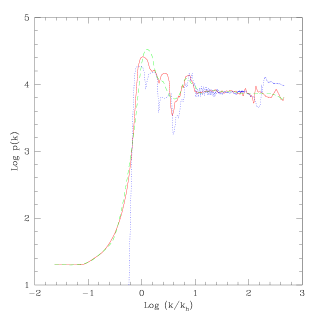
The original primordial power spectrum which we use in this paper (see figure 1) is the final recovered primordial power spectrum obtained in Ref. prd04 for a flat $\Lambda$CDM cosmological model with $\tau$=0.0, $h$=0.71, $\Omega_{b}h^{2}$=0.0224 and $\Omega_{\Lambda}$=0.73. The resultant $C_{l}$ spectrum using this recovered spectrum has a likelihood far better than a scale invariant or a best fit power law spectrum. In this paper, we investigate how the features of this spectrum contribute to improving the likelihood.

The blue dotted line in figure 1 represents the recovered primordial spectrum by using WMAP-3 data which gives $\Delta\chi^{2}_{eff}=-15.93$ (by using WMAP-3 likelihood code) with respect to the best power law primordial spectrum in the whole cosmological parameter space. In this paper we are not using this recovered spectrum for our wavelet analysis and it has been presented here just to show the close similarity of the features of the recovered spectrum from WMAP-1 and WMAP-3 data.

First, we smooth the spectrum using DWT, and then we systematically include features at different resolutions and calculate the likelihood with respect to the WMAP data.

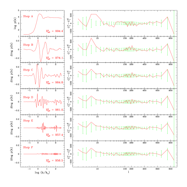
In figure 2, left panel (step A), we show the coarsest behavior of the data reconstructed using only the 10th level low-pass coefficients. The right panel shows the resultant $C_{l}^{r}$ compared with the observed binned data $C_{l}^{d}$, and its error bars. The likelihood of the $C_{l}^{r}$ at this stage corresponds to $\chi^{2}_{\rm eff}=994.4$ which is better than the $\chi^{2}_{\rm eff}$ for the H-Z spectrum. In the right panel (step B) we see that if we include ‘low frequency’ features as captured by the 10th level high-pass coefficients shown in the left panel (step B) to the previous spectrum at step A, the resultant $C_{l}^{r}$ will be closer to the observed data. Hence we expect the likelihood to be improved. In fact this improves the likelihood significantly and the $\chi^{2}_{\rm eff}=974.1$ at this stage (the reconstructed spectrum is the green-dashed line in figure 1). This $\chi^{2}_{\rm eff}$ is better than the best fit power law spectrum with the $\chi^{2}_{\rm eff}=978.6$.

As we progressively add back more features at ‘higher frequencies’ to the spectrum the likelihood improves significantly. The 9th, 8th, 7th and 6th level wavelet coefficients are shown in the left column of figure 2 (steps $C,D,E$ and $F$). The plots in the right panel of figure 2 show how we get closer to the observed data within the error bars as we include more wavelet coefficients. The likelihoods at these steps correspond to are $\chi^{2}_{\rm eff}=964.8$ at step $C$, $\chi^{2}_{\rm eff}=961.0$ at step $D$, $\chi^{2}_{\rm eff}=957.4$ at step $E$, and $\chi^{2}_{\rm eff}=956.5$ at step $F$.

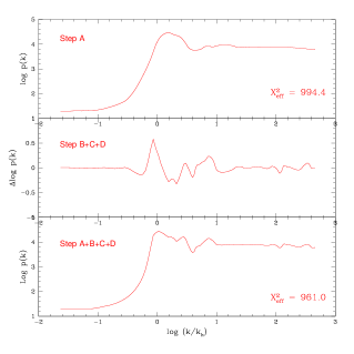
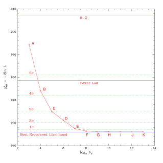
In figure 3 we compare the coarsest spectrum of step $A$ and the spectrum after adding the features of step $B$, $C$ and $D$. The local features which are responsible for the significant improvement of the likelihood are clearly seen. We note that most of these features are localized around the horizon scale. In figure 4, we see that after few stages of adding the more detailed features to the spectrum, the likelihood does not improve anymore and agreement with the observed data is not sensitive to these features.

V Conclusion

This paper presents a detailed analysis of the recovered primordial power spectrum for a flat $\Lambda$CDM cosmological model, given in Ref. prd04 . The recovered spectrum has a likelihood far better than a simple scale invariant or a scale free spectra. In Ref. bump05 , similar features for the primordial spectrum have been detected by using a completely different method and the significance of the features have also been evaluated. In this paper we use Discrete Wavelet Transform to decompose the features of the spectrum to quantify and understand their role in improving the likelihood. In addition to the infra-red cut-off around the horizon, which was proposed by many groups to explain the lack of power in very low multipoles of the observed angular power spectrum, we show that the features around the horizon are playing a crucial role in improving the likelihood. In fact, the effect of these features on improving the likelihood, are very significant (figure  3). We find that these strong features are localized around the horizon. Work on WMAP 3 years data is in progress and will be reported in a forthcoming publication armarun06 . The work in progress implies refinement of methodology includes directly employing DWT right at the stage of smoothing the raw recovered spectrum and dispensing with the need to remove a ‘template’ spectra as in Ref. prd04 .

VI Acknowledgment

We thank S. Hemachander and S. Nanavathy for their contribution in the early stages of this work. We acknowledge the use of the Legacy Archive for Microwave Background Data Analysis (LAMBDA). Support for LAMBDA is provided by the NASA Office of Space Science.

References

- (1) A. Shafieloo and T. Souradeep, Phys Rev. D 70, 043523 (2004).
- (2) A. A. Starobinsky, Phys. Lett, B 117, 175 (1982).
- (3) A. H. Guth and S.-Y. Pi, Phys. Rev. Lett., 49, 1110 (1982).
- (4) J. M. Bardeen, P. J. Steinhardt, M. S. Turner, Phys. Rev. D 28, 679 (1983).
- (5) U. Seljak. et al., Phys. Rev. D 71, 103515 (2005).
- (6) D. Spergel et al., Astrophys.J.(in press), (astro-ph/0603449).
- (7) L. Covi. et al., Phys. Rev. D 74, 083509 (2006).
- (8) H. Peiris and R. Easther, preprint, (astro-ph/0609003).
- (9) M. Bridges, A. Lasenby, M. Hobson, Mon.Not.Roy.Astron.Soc. 369 B1123 (2006).
- (10) J. Martin and C. Ringeval, J. Cosmo. Astropart. Phys. 0608 009 (2006).
- (11) S. L. Bridle et. al., Mon.Not.Roy.Astron.Soc. 342 L72 (2003).
- (12) S. Hannestad, J. Cosmo. Astropart. Phys. 0404, 002 (2004).
- (13) P. Mukherjee and Y. Wang, Astrophys.J. 599 1 (2003).
- (14) P. Mukherjee and Y. Wang, J. Cosmo. Astropart. Phys. 0512 007 (2005).
- (15) S. Leach, Mon.Not.Roy.Astron.Soc. 372 L646 (2006).
- (16) M. Tegmark and M. Zaldarriaga, Phys. Rev. D66, 103508, (2002).
- (17) M. Matsumiya, M. Sasaki, J. Yokoyama, Phys. Rev. D65, 083007, (2002); ibid, JCAP 0302 003 (2003).
- (18) A. Shafieloo, T. Souradeep. In preparation.
- (19) D. Tocchini-Valentini, Y. Hoffman, J. Silk, Mon.Not.Roy.Astron.Soc. 367 T1095 (2006).
- (20) N. Kogo, M. Matsumiya, M. Sasaki, J. Yokoyama Astrophys.J. 607 32 (2004).
- (21) C. Contaldi et al., J. Cosmo. Astropart. Phys. 0307, 002 (2003).
- (22) N. Kaloper and M. Kaplinghat, Phys. Rev. D 68, 123522 (2003).
- (23) M. Kawasaki, F. Takahashi and T. Takahashi, Phys. Lett, B 605, 223 (2005).
- (24) P. Hunt, S. Sarkar, Phys. Rev. D70, 103518, (2004).
- (25) S. Sarkar, Nucl. Phys. B148 1 (2005)
- (26) R. Sinha and T. Souradeep, Phys. Rev. 74, 043518, (2006).
- (27) N. Barnaby, J. M. Cline, Phys. Rev. D73, 106012, (2006).
- (28) A. Ashoorioon, A. Krause preprint, (hep-th/0607001).
- (29) L. B. Lucy, Astron. J., 79, 6 (1974).
- (30) B. H. Richardson, J. Opt. Soc. Am., 62, 55 (1972).
- (31) C. M. Baugh and G. Efstathiou, Mon.Not.Roy.Astron.Soc. 265, 145 (1993).
- (32) C. M. Baugh and G. Efstathiou, Mon.Not.Roy.Astron.Soc. 267, 323 (1994).
- (33) We can dispense with the step of removing a template employed in Ref. prd04 to remove the artifacts at low and high wavenumber with a small change in our algorithm armarun06 .
- (34) I. Daubechies, Ten Lectures on Wavelets, SIAM, Philadelphia, PA, 1992. Vol.64, CBMS-NSF Conference Series in Applied Mathematices.