Abstract

Adaptive optics systems are essential on all large telescopes where image quality is important. These are complex systems with many design parameters requiring optimisation before good performance can be achieved. The simulation of adaptive optics systems is therefore necessary to categorise the expected performance. This paper describes an adaptive optics simulation platform, developed at Durham University, which can be used to simulate adaptive optics systems on the largest proposed future extremely large telescopes (ELTs) as well as current systems. This platform is modular, object oriented and has the benefit of hardware application acceleration which can be used to improve the simulation performance, essential for ensuring that the run time of a given simulation is acceptable. The simulation platform described here can be highly parallelised using parallelisation techniques suited for adaptive optics simulation, whilst still offering the user complete control while the simulation is running. Results from the simulation of a ground layer adaptive optics system are provided as an example to demonstrate the flexibility of this simulation platform.

OCIS codes: 010.1080, 010.7350

1 Introduction

Adaptive optics (AO) is a technology widely used in optical and infra-red astronomy, and almost all large science telescopes have an AO system. A large number of results have been obtained using AO systems which would otherwise be impossible for seeing-limited observations[1, 2]. New AO techniques are being studied for novel applications such as wide-field high resolution imaging [3] and extra-solar planet finding [4].

The simulation of an AO system is important as it helps to determine how well the AO system will perform. Such simulations are often necessary to determine whether a given AO system will meet its design requirements, thus allowing scientific goals to be met. Additionally, new concepts can be modelled, and the simulated performance of different AO techniques compared[5], allowing informed decisions to be made when designing or upgrading an AO system and when optimising the system design parameters.

A full end-to-end AO simulation will typically involve several stages [6]. Firstly, a representation of the atmospheric turbulence is produced, typically by generating simulated atmospheric phase screens, often using several different screens representing turbulence at different atmospheric heights. The aberrated complex wave amplitude at the telescope aperture is then generated by modelling this atmospheric phase as seen from the telescope pupil. For a stratified atmospheric model, this will involve propagating the atmospheric phase screens across the pupil, to simulate the effect of the relative velocity of different atmospheric layers. The wavefront at the pupil is then passed to the simulated AO system, which will typically include one or more wavefront sensors and deformable mirrors and a feedback algorithm for closed loop operation. Additionally, one or more science point spread functions (PSFs) as corrected by the AO system are calculated. Information about the AO system performance is computed from the PSFs, including quantities such as the Strehl ratio and encircled energy.

The computational requirements for AO simulation scale rapidly with telescope size, and so simulation of the largest telescopes cannot be done without special techniques, some of which follow:

1. Multiprocessor parallelisation [7, 8] allows computations to be spread across multiple processors, though can suffer from data bandwidth bottlenecks, as often data cannot be transferred between processors at a rate sufficient to keep them processing for a large proportion of the time.

2. The use of dedicated hardware for algorithm acceleration [9] can produce large performance improvements, though is somewhat inflexible.

3. Analytical models can also be used [10], and these can give rapid results, though are not able to represent noise sources easily.

We here describe the approaches that we have taken to implement an efficient and scalable simulation framework.

1.A The Durham adaptive optics simulation platform

At Durham University, we have been developing AO simulation codes for over ten years [11]. The code has recently been rewritten to take advantage of new hardware, new software techniques, and to allow much greater scalability for advanced simulation of AO systems for extremely large telescopes (ELTs), including multi-conjugate AO (MCAO) and extreme AO (XAO) systems [12].

The Durham AO simulation platform uses the high level programming language Python (currently, Python 2.4), to select and link together C (ANSI standard with GCC version 3.3), Python and hardware accelerated algorithms, as well as third party modules, giving a great deal of flexibility. This allows us to rapidly prototype and develop new and existing AO algorithms, and to prepare new AO system simulations quickly using Python code. The use of C and hardware algorithms ensures that processor intensive parts of the simulation platform can be implemented efficiently. The C and Python algorithms make use of optimised libraries including FFTW (versions 2 and 3), the AMD core math library (version 3.5, for use on AMD platforms, including BLAS and LAPACK routines), the GNU scientific library (currently version 0.7), and the MPICH library (optimised for the Cray XD1). This ensures that high performance can be achieved for computationally intensive algorithms. The hardware accelerated algorithms are implemented within field programmable gate arrays (FPGAs), which can be programmed to provide impressive performance improvements over a standard software implementation. The VHDL hardware description language is used to program the FPGAs, using the Xilinx ISE 7.1 compiler.

The simulation software will run on most Unix-like operating systems, including Linux and Mac OS X. The simulation platform hardware at Durham consists of a Cray XD1 supercomputer [13], which contains reprogrammable hardware for application acceleration as well as six dual Opteron processor nodes each with 8 GB ram. Additionally, a distributed cluster of conventional Unix workstations is connected by giga-bit Ethernet. For most simulation tasks, only the XD1 is required, though for large models, or when multiple simulations are run simultaneously, the entire distributed cluster can be used. The simulation is programmed intelligently to make use of optimised libraries and hardware acceleration when these are available, and to use default library replacements when not (for example, the AMD core math library is not available on a Mac OS X platform).

The simulation is object orientated, with high level objects (for example a phase screen generation object, and a wavefront sensing object) being connected together, allowing data to be passed between them in a direction described by the user (for example, atmospheric phase screens may be passed to a deformable mirror object). The high level simulation objects can contain instances of lower level objects, which are internal to the simulation objects, and used during calculations, for example a telescope pupil mask object, used to define which parts of the atmospheric phase screens are sampled by the wavefront sensor.

2 ELT simulation requirements

When attempting to create a realistic simulation of an AO system on an ELT, a large amount of computing power, memory and bandwidth will be required. The Durham simulation platform provides these requirements by implementing several key technologies.

2.A Multiple processor simulation platform

The Durham simulation platform allows a simulation to be comprised of multiple processes, meaning that different parts of the simulation can run on different processors, and even different computers. This however means that communication between the processes is essential. To maximise the efficiency of the simulation, we use a combination of shared memory access (where processes have access to the same memory, e.g. within a symmetric multiprocessor (SMP) system), and message passing interface (MPI) communications where appropriate, and a simulation user has control over the type of communication used.

2.A.1 Shared memory access

Shared memory access allows multiple processes to access the same region of computer memory. All processes can usually have read and write access to this memory. Using shared memory allows a single memory block to be shared between processes, thus reducing the overall memory requirements, and also reducing the processor overhead, as producing an identical copy of the data for each different processes is then not essential. Fig. 1 is a schematic diagram showing how a typical shared memory system can operate. Shared memory buffers are created using the Unix shm_open() function call, and are mapped into a processors virtual address space. Standard synchronisation primitives, such as semaphores are used to ensure that no processes are reading the shared memory region whilst it is being written to, and to ensure that only one process can write to the shared memory region at once.

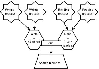
Fig. 1: A schematic diagram showing how a typical shared memory system will operate. Some processes will have read and write access to the memory, while others will have read access only. Synchronisation primitives will be used to ensure that data is not read while it is being written and vice versa.

The Durham simulation platform hides the use of synchronisation primitives (in this case, semaphores) from the user (and simulation objects), such that the parallel processes will read and write to the shared memory region only when it is appropriate to do so. This removes the possibility of data corruption, whilst providing a simplified interface for the simulation programmer.

2.A.2 MPI communication

Communication between distributed systems which do not share memory requires copies of datasets to be passed between the systems. When the dataset is large, or when a large number of small datasets are passed, a bottleneck can occur as processes will then spend a significant amount of time waiting for a dataset to arrive or be sent. It is therefore essential that the communication method used to transfer these datasets is as efficient as possible, having both a low latency (so that time is not wasted when sending small datasets), and a high sustained bandwidth (so that large datasets can be sent in a minimum time).

The Durham simulation platform uses the MPI library for this communication, as this allows data to be passed efficiently with only a small latency, particularly on the XD1 system. The Cray XD1 has an optimised version of the MPI library which is targeted to the hardware architecture of this system, making efficient use of the RapidArray Transport interface, the commercial high bandwidth interconnect found in XD1 systems. Using the Durham system, we have measured the MPI communication latency of only 1.6 $\mu$s, and a maximum sustained bandwidth of 1.4 GBs^-1 between the computing nodes.

2.A.3 Process parallelisation

Each processor used for a given simulation will be given only one process to run, to reduce context switching delays. Each of these processes will contain one or more simulation objects, which are able to access the virtual memory space of other objects within the process, making data transfer between these objects trivial (e.g. the address of a data array can be passed). All simulation objects are executed in a single thread, carrying out their computations for each iteration in turn, which again reduces context switching delays.

Objects in separate processes are able to pass data using either MPI communications or shared memory as appropriate. When such communication is required, a pair of high level communication objects are created and are responsible for dealing with a particular communication link (MPI or shared memory). These communication objects are then connected to the simulation objects, which can then behave as if they are connected directly to the object with which they wish to communicate. Each simulation object has a basic set of methods and data objects which are viewable by other objects. The communication objects then merely have to implement these methods and data objects, transferring data as appropriate. The use of communication objects is transparent to the simulation objects, being handled by the simulation framework.

2.B Hardware acceleration

The Durham AO simulation platform is able to accelerate specific parts of the AO simulation by using reconfigurable logic hardware, FPGAs, and hence reducing the time taken for a given simulation to complete. These FPGAs are an integrated part of the Cray XD1 supercomputer [9] and when used correctly, are capable of reducing the execution time of some algorithms by two to three orders of magnitude[14], whilst at the same time, freeing the CPU for other operations. This greatly improves the speed at which the simulation can run, and is essential for simulation of large AO systems. Implementing algorithms within the FPGAs requires knowledge of a hardware programming language, and so we have developed common libraries which can be plugged in to an existing simulation, for example a wavefront sensor pipeline. The simulation user therefore requires no hardware knowledge, and yet can achieve significant impressive performance improvements using the hardware acceleration.

2.C Simulation creation

A user creates a new simulation by selecting and linking together the various simulation modules as required, either graphically or in a text file. New modules (for example to investigate a new type of wavefront sensor or deformable mirror) can easily be created and added to the simulation with minimal effort. Once the simulation file has been set up, a parameter file is created which contains all variables and configuration objects required by the simulation. This parameter file is in XML format and allows embedded Python code which can be used to create complicated variables and objects. If suitably defined, a cross-simulation parameter file could be created using a Python parser for the XML. The parameter file can be created using a graphical interface, which has the capability to automatically create a skeleton parameter file from the simulation file, and then allow the user to adjust the default values of variables. This allows a new simulation to be set up quickly by an inexperienced user.

2.D Simulation control

Control of a running simulation is achieved by connecting to it using either the Python command-line or graphical tools. This gives the user complete control over a simulation, allowing them to stop, start and pause, as well as analyse (allowing the user to create plots of parts of the data chain, for example, sub-aperture images) and change the current state of a simulation (for example, changing the value of a variable or the contents of an array). This high degree of flexibility is achieved by allowing the user to send text strings to the simulation, which are treated as Python code, and executed as a separate thread which has access to the global name-space. The user can therefore access and alter any part of the simulation, and any requested data can be returned to the user for further analysis. When a simulation is comprised of more than one process, the user can connect to any or all of these processes.

This control facility is completely detachable from the simulation, and can be started and stopped without affecting simulation operation. It is also possible to have several users connected to the same simulation at any given time, from anywhere that has Internet access to the computers running the simulation. Fig. 2 shows a screen-shot of the simulation control user interface, and demonstrates the powerful functionality that this provides through a simple interface, satisfying both novice and experienced users.

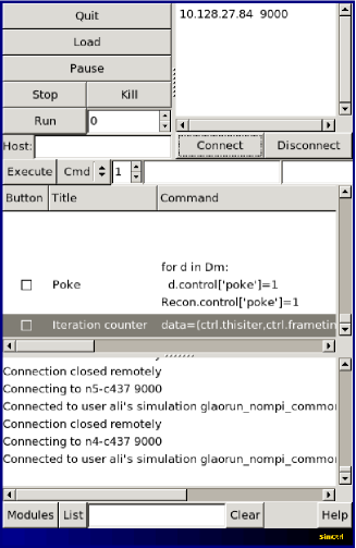
Fig. 2: A screen-shot of the simulation control user interface. Novice users are able to control a simulation at the click of a button, while experienced users are able to query the simulation, obtain and display data, and alter the simulation state, including changing values and array contents.

This simulation control capability is unique as it enables a user to implement new capability within a running simulation, and to query all objects and variables, even if it was not envisaged that these should be queried before the simulation was created. This high degree of flexibility is essential for ELT AO system simulation as simulation run-times can typically be measured in days.

2.E Parallelisation approaches

When parallelising any software, there is usually a trade off between the amount of processing done, and the amount of data that has to be passed between processors. A bottleneck may occur if the CPUs spend a significant amount of time waiting for data, meaning that the parallelisation has not been efficient.

It is usually most efficient to create parallelised software which sends as little data as possible between processes so that most time can be spent processing data. At Durham, we typically parallelise our AO system simulations by dividing parallel optical paths into separate processes, as shown in Fig. 3. Each optical path is virtually independent of the others, except that they all require inputs of atmospheric phase screen data and knowledge of any time varying deformable mirror surface shapes, and may (if part of the wavefront correction path) return new deformable mirror commands, or wavefront sensed values to be passed to other optical paths. By dividing the processes in this way, a minimum amount of time is spent waiting for data, allowing the most efficient use of the CPUs to be made. This will also allow a typical simulation (with several on and off-axis science targets, and one or more guide stars) to be parallelised into a similar number of processes as there are processors, allowing a single process to run on each processor.

When all parallel optical paths depend on one algorithm which generates data for the paths, for example, atmospheric turbulence generation, or reconstruction of the deformable mirror commands from the wavefront sensor data, this algorithm can also be parallelised using a traditional parallelisation approach, by splitting the computation over available processors, and passing the data as required. Some optimised libraries, for example the FFTW Fourier transform library, use this technique. However, this parallelisation approach is only beneficial for algorithms where the time spent transferring data is small compared with the time spent processing the data.

Fig. 3: An example of the parallelisation of parallel optical paths. No data-flow is required between these paths, except for the initial phase screens, meaning that minimal time is spent with the processors waiting for data to arrive.

2.E.1 Simulation scalability

To demonstrate the scalability of the AO simulation, we have simulated a system with three wavefront sensors ($32\times 32$ sub-apertures each), one science target, and assume that atmospheric turbulence is concentrated in two layers. Table 1 provides details of the different simulation objects required for this simulation, and gives typical computation times for this example. It should be noted that the computation times do not scale identically with simulation size, and so the ratio of computation times between different algorithms is not constant for larger or smaller simulations.

We demonstrate the strong scalability of the AO simulation platform by keeping the simulation a fixed size, but increasing the number of processors that are used. Table. 2 shows the simulations parallelised by placing different simulation objects on different processing nodes. For the small simulation used for this demonstration, this type of parallelisation can be sub-optimal, because the processing load can be poorly balanced between processors. For example, when placed on two processors, one of these will have two wavefront sensor objects, requiring approximately double the processing time of the other processor (with only one wavefront sensor object).

By parallelising some of the simulation objects (in this case the wavefront sensing objects), the computational load can be spread more evenly across processors, thus giving a better performance scaling with computer system size. Table. 3 shows the simulations parallelised by using parallelised wavefront sensing objects, allowing a better fit to a greater number of processors to be realised as the processing load can be distributed more evenly. The timing results for these simulations are shown in Fig. 4. This figure shows that the simulation can scale well when it is well suited to the number of processors, for example, using three processors gives a simulation rate three times greater than one processor. However, when the simulation is not well suited to the number of processors (for example 2, 4, 5 and 6 processors in the case when the individual simulation objects are unparallelised), the performance is sub-optimal. If individual objects are parallelised, the simulation can be fitted better to the number of available processors, as the dotted line in Fig. 4 shows. However, currently, not all simulation objects can be parallelised.

Simulation object	Significant algorithms	Computation time / s
Infinite phase screen generation	Matrix operations	$10^{-4}$
Atmospheric pupil phase	Matrix operations	$7\times 10^{-4}$
Deformable mirror simulation	Matrix operations	0.03
Shack-Hartmann sensor, slope computation	FFT, matrix operations	0.18
Wavefront reconstruction (SOR)	Matrix operations	0.02
Science image generation	FFT, matrix operations	0.02

Table 1: A table describing the simulation objects used in a study of the AO simulation strong scalability.

ONE CPU CONFIGURATION	TWO CPUs		THREE CPUs			FOUR CPUs
CPU1	CPU1	CPU2	CPU1	CPU2	CPU3	CPU1	CPU2	CPU3	CPU4
1. Phase screen (2km)	1.	4.	2.	4.	1.	2.	1.	4.	5.
2. Phase screen (0km)	2.	5.	3.	7.	5.	3.	3.	7.	8.
3. Telescope pupil phase (direction 1)	3.	7.	6.	10.	8.	6.	6.	10.	11.
4. Telescope pupil phase (direction 2)	6.	8.	9.	12.	11.	13.	9.
5. Telescope pupil phase (direction 3)	9.	10.	13.			12.
6. Deformable mirror (direction 1)	13.	11.
7. Deformable mirror (direction 2)	12.
8. Deformable mirror (direction 3)
9. Wavefront sensor (direction 1)
10. Wavefront sensor (direction 2)
11. Wavefront sensor (direction 3)
12. Wavefront reconstructor
13. Science calculation (science image)

Table 2: A table showing how simulation objects can be placed on different computing nodes to parallelise a simulation. The first column gives a brief description of each object, the numbers of which are then referred to in other columns.

ONE CPU		TWO CPUs		THREE CPUs			FOUR CPUs				SIX CPUs
CPU1		CPU1	CPU2	CPU1	CPU2	CPU3	CPU1	CPU2	CPU3	CPU4	CPU1	CPU2	CPU3
1.	2.	1.	2.	2.	4.	1.	1.	2.	5.	10.c	1.	2.	5.
3.	4.	4.	5.	3.	7.	5.	3.	4.	8.	10.d	3.	4.	8.
5.	6.	7.	8.	6.	10.a	8.	6.	7.	11.a	11.d	6.	7.	11.a
7.	8.	3.	10.c	9.a	10.b	11.a	9.a	9.d	11.b		9.a	10.a	11.b
9.a	9.b	6.	10.d	9.b	10.c	11.b	9.b	10.a	11.c		9.b	10.b
9.c	9.d	9.a	11.a	9.c	10.d	11.c	9.c	10.b	12.		13.
10.a	10.b	9.b	11.b	9.d	12.	11.d	13.				CPU4	CPU5	CPU6
10.c	10.d	9.c	11.c	13.							9.c	10.d	11.d
11.a	11.b	9.d	11.d								9.d	10.d	11.d
11.c	11.d	10.a	12.									12.
12.	13.	10.b
		13.

Table 3: A table showing how the parallelisation of simulation objects (denoted here by a, b, c and d suffixes for a four way parallelisation of the wavefront sensing algorithm) can be used to fit a simulation to a given number of CPUs. The numbers represent the simulation objects described in table 2

Fig. 4: A figure showing the number of simulation time-steps computed per unit time (simulation rate) when the simulation is parallelised over different numbers of processors. The solid line shows the case when individual objects are not parallelised, while the dotted line shows the case when the Shack-Hartmann image creation and wavefront sensing algorithm is parallelised, providing a better fit to larger numbers of processors. The simulation rate has been normalised to unity by the rate for an unparallelised simulation (with unparallelised simulation objects).

2.F ELT simulation suitability

The Durham AO simulation platform is suited for the simulation of ELT scale AO systems. The XD1 supercomputer has 8 GB memory per computing node, allowing large phase-screens, large numbers of wavefront sensing elements (for example, Shack-Hartmann sub-apertures), and other data to be stored. The tight integration of the FPGAs with memory and CPUs means parts of the simulation can be accelerated by several orders of magnitude, and the high bandwidth, low latency connections between nodes allows data to be passed rapidly between parallelised processes. This simulation platform provides the capability for rapid simulation of AO systems on all current telescopes and next generation ELTs.

2.F.1 ELT simulation details

A simulation of a classical AO system on an ELT has been created to demonstrate the use of the AO simulation platform. The key parameters of this simulation are detailed in table 4. This simulation uses an infinite phase screen generator with von Karman statistics [15]. A successive over-relaxation (SOR) wavefront reconstructor is used, which means that it is not necessary to create and invert an interaction matrix of the system. In a system of this size, a full interaction matrix could easily take more memory than available on our Cray XD1 system, also taking a prohibitive length of time (days or weeks) to invert to obtain the control matrix, and so conventional wavefront reconstruction is not an option. We are currently implementing sparse matrix algorithms and Fourier domain wavefront reconstruction algorithms which will greatly reduce the memory and computation requirements. An FPGA hardware accelerator is used for computation of the Shack-Hartmann images, and the spot centroid location algorithm. The high number of pixels per sub-aperture allows elongated Shack-Hartmann spots (e.g. from a laser guide star) to be analysed. The simulation includes one wavefront sensor, and one science target. A more useful simulation may include several wavefront sensors and several science targets, though these are not presented here.

Simulation parameter	Value
Telescope primary	42m
Atmospheric layers	3 (0 km, 2 km, 10 km)
Wavefront sensors	1
Number of sub-apertures	$256\times 256$ (16 cm per sub-aperture)
CCD pixels per sub-aperture	$16\times 16$
Deformable mirrors	1
Number of deformable mirror actuators	$256\times 256$
Atmospheric resolution	1 cm of sky per phase pixel
Phase pixels for science image creation	$4096\times 4096$
Guide stars	1 (natural guide star)

Table 4: A table showing the ELT simulation model details

This simulation has been parallelised over five nodes of the Cray XD1, one node for each atmospheric layer, one node for the science target, and one node to combine the atmospheric layers to give the atmospheric phase at the telescope pupil, perform the simulation of the wavefront sensor, and reconstruct the wavefront allowing the deformable mirror surface to be reshaped. Table 5 shows the relative time spent computing each of these algorithms, and it can be seen that by far the most computationally intensive is the simulation of the science target (involving a $8192\times 8192$ fast Fourier transform for each simulation time-step). These timings are pessimistic (worse case), as they include computation of all scientific parameters, including Strehl ratio and enclosed energy, which would typically only be performed every hundred or so time-steps. Without these calculations, the science object takes less than 50 seconds to compute and store the instantaneous point spread function for this ELT simulation. It should be noted that these timings do not scale in the same way as a function of system size; for example when simulating a smaller telescope, computation of the science image takes a significantly smaller fraction of processor time.

For the majority of the time, the other processors are idle, waiting for the science image algorithm to complete. Work is currently underway to place the bulk of this algorithm into hardware, which will result in a significant performance improvement (a factor of 10 times is expected). The computation time of the science target simulation currently scales as $O(n^{2}\log n)$, due to the large two dimensional fast Fourier transform, where $n$ is the linear size of the phase screen (measured in pixels). This algorithm also uses the most memory as it has to store a zero-padded pupil phase (so that the Fourier transform is sampled at the Nyquist frequency), and both an instantaneous and integrated point spread function. The memory requirements for this algorithm scale as $O(n^{2})$ where $n$ is the linear size of a phase screen, and over 5 GB memory were required for this algorithm in the example here. With the current hardware, it would be possible to create a simulation with one more science object (on the currently spare processing node), and about six more wavefront sensing objects, to create (for example) a MCAO simulation, without increasing the simulation iteration time. This has not been implemented at the present time, as the MCAO wavefront reconstructor is not yet complete.

Algorithm	Time taken / s
Science image and statistics	70
Atmospheric pupil phase	6.1
Deformable mirror	2.8
Wavefront sensing (Shack-Hartmann sensor, slope computation)	0.6
Wavefront reconstruction (SOR)	2.0
Phase screen generation	2.9 per layer

Table 5: A table showing the time spent in each algorithm of the ELT simulation. The time taken for each simulation iteration (corresponding to 5 ms real time) was about 70 seconds, limited by the time to perform the science image computation.

The planet finder instrument for the European Southern Observatory ELT project is currently specified to have $200\times 200$ sub-apertures [16], and this is one of the most demanding proposals. The simulation demonstrated here is therefore of higher order (has a larger number of sub-apertures) than all present and planned astronomical AO systems.

3 Simulation results for ground layer adaptive optics

A classical or single guide star AO system can produce only a small corrected field of view, and isoplanatic errors cause the image quality to quickly degrade from the centre of this field. When natural guide stars are used, the sky coverage for these AO systems is severely limited, since it is difficult to find stars that are bright enough within each isoplanatic patch of sky. Ground layer AO (GLAO) was proposed as a solution to this problem, by applying a limited AO correction for a large field of view under any atmospheric conditions at optical and infra-red wavelengths [17]. A GLAO system is not designed to produce diffraction limited images, but improves the concentration of the PSF by correcting only the lowest turbulent atmospheric layers. Correction is then virtually identical over the entire field of view since these layers are closer to the ground, while the uncorrected higher layers degrade the spatial resolution isoplanatically.

At Durham, we have implemented a GLAO simulation model using the AO simulation framework for corrected fields up to 15 arc-minutes in size based on high resolution turbulence profiles taken at the Gemini observatory [18], and some of the results are presented here to demonstrate an actual use of the simulation. The Durham simulation model includes detailed wavefront sensor (WFS) noise propagation and produces 2D PSFs, and is used to quantify the effects of such noise on the PSF parameters across the GLAO field for various seeing and noise conditions. The capabilities of this model are summarised:

1. The atmosphere can be modelled as any number of independently moving turbulent layers.

2. Multiple laser beacons and guide stars can be modelled.

3. Multiple deformable mirrors of different types can be modelled.

4. Multiple wavefront sensors can be included, encompassing all main detector noise effects, pixellation and atmospherically induced speckle.

5. The science PSF can be sampled at any number of field points simultaneously.

It is wholly-independent code (not derived from any other simulation platform), but can be used subject to detailed cross-checks with other AO models [18]. This checking has been carried out as part of work for the Gemini telescope consortium. The simulation can also be used for situations where the atmosphere cannot be treated as stratified in layers, but as a three dimensional entity simply by implementing such a model. However, this is not considered here.

3.A Durham implementation

A design for the GLAO system is shown in Fig. 5, and this indicates that there are multiple guide stars and multiple science sampling points where the AO system performance is categorised.

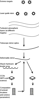
Fig. 5: A figure showing the design of a GLAO system.

We have simulated a system with five laser guide stars, and four discrete atmospheric turbulence layers as shown in table 6, assuming an 8 m telescope primary mirror. The simulation takes samples of the science field at a wavelength of 1250 nm at ten positions, on and off-axis, as well as the uncorrected image, and uses these samples to categorise the performance of the AO system, with parameters such as the Strehl ratio and encircled energy being computed for each science target location. The simulation uses a Shack-Hartmann wavefront sensor with $10\times 10$ sub-apertures, and assumes a generic deformable mirror to which combinations of Zernike modes are applied to give the correct mirror shape at each time-step (the first 54 Zernike modes were corrected). A typical layout of the science stars and guide stars is shown in Fig. 6, as viewed from the telescope. The guide star angle from the on-axis direction can be varied between 200–750 arc-seconds, and this can be used to investigate the degree of AO correction, and the area over which this correction is achieved. The integrated seeing in these models was taken as 0.6 arc-seconds with a Fried parameter of 0.17. An exposure time of 100 seconds was used with a WFS integration time of 2 ms. The laser guide stars were assumed to be of 13th magnitude brightness.

Layer height / m	0	300	2000	10000
Wind speed / ms-1	6	9	10	18
Relative layer strengths	0.45	0.15	0.07	0.33

Table 6: A table showing the atmospheric model details

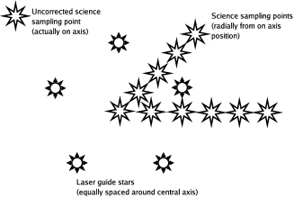
Fig. 6: A schematic diagram of the relative positions of the laser guide stars and science sampling points used for the GLAO simulation. The science sampling points (larger stars) are spaced uniformly 150 arc-seconds apart, while the laser guide stars (smaller stars) are positioned equally around a circle with a diameter which can be varied between 200–750 arc-seconds.

3.B Parallelisation approaches

There are many ways in which a large simulation such as that presented here can be parallelised. The optimal parallelisation approach will reduce the bottlenecks in data transferred between processes and minimise the amount of time in which processors are not actively processing, whilst fully utilising as many processors as possible. As mentioned in section 2.E, when simulating an AO system, it is possible to separate the parallel optical paths from different guide stars and science targets on to different processors, reducing the data transfer between processes. This is the approach used here, and is presented as a flowchart in Fig. 7.

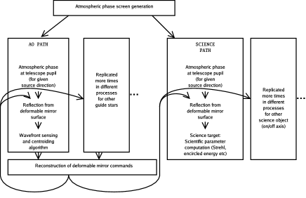
Fig. 7: A flowchart showing how the GLAO simulation is carried out using the Durham AO simulation platform. The algorithms in different boxes are implemented on different processors, and arrows show the direction of data flow between the algorithms. Typically, there will be between 5 and 10 science paths (to determine how the AO performance changes at different angles from the vertical axis), and between 5 and 10 AO paths, depending on the number of laser guide stars being used.

3.C GLAO simulation results

When a number of guide stars are evenly spaced about a circle (as viewed from the telescope), there will be some atmospheric correction for starlight passing within this circle, but the degree of correction will fall for starlight outside the circle. If the guide star separation is reduced, better correction will be achieved over a smaller area. Conversely, if the separation is increased, a poorer correction will be achieved over a larger area.

A GLAO system does not aim to achieve a high degree of correction. Rather, a partial degree of correction is achieved over a wide field of view, and the GLAO system is usually designed to be complementary to more conventional AO systems, or to be used with integral field spectroscopy units. The correction achieved from a GLAO system alone typically produces Strehl ratios of only a few percent.

The results of an investigation into the effect of guide star separation are presented here, and Fig. 8 shows that by moving the guide stars out from the on-axis direction, the isoplanatic correction covers a larger area with a smaller degree of correction, hence giving a lower Strehl ratio. This decreases for fields further from the on-axis direction, but the rate of change is dependent on the guide star separation. The uncorrected Strehl ratio was about 0.75 percent.

Fig. 8: A figure showing the Strehl ratio as a function of distance from the on-axis direction. The solid line is for a laser guide star separation of 700 arc-seconds from the on-axis direction, the dotted line for a separation of 550 arc-seconds, the dashed line for a separation of 450 arc-seconds and the dot-dashed line for a separation of 250 arc-seconds. The points and error bars are obtained from a sample of 10 results for each point.

The full width half maximum (FWHM) as a function of angle from the on-axis direction also displays the expected behaviour, increasing as the viewing angle is moved away from the axis. When the guide star separation is small, the FWHM is small close to the axis, increasing rapidly away from it, and when guide star separation is large, the FWHM is initially larger, but increases slowly away from the on-axis direction, as shown in Fig. 9. The uncorrected FWHM was 0.35 arcsec.

Fig. 9: A figure showing the change in the FWHM of corrected images as a function of angle from the on-axis direction. The solid curve is calculated with a guide star angle of 700 arc-seconds from the axis, the dotted curve for 550 arc-seconds, the dashed curve for 450 arc-seconds and the dot-dashed curve for 250 arc-seconds.

The GLAO simulation presented here has been compared with other independent AO simulation codes [18], and are found to be in agreement within the statistical uncertainties.

4 Conclusion

We have developed a new AO simulation capability at Durham for astronomical applications, and this platform is capable of extremely large telescope AO system simulation. This simulation platform is capable of using algorithms implemented within reconfigurable logic to provide hardware acceleration for the most computationally intensive tasks.

A simulation platform includes tools for creating and controlling the simulations, and optimal parallelisation techniques specific to AO simulations have been discussed. The flexibility of the simulation platform, as well as the ability to query and alter the state of a running simulation make it unique. Additionally, techniques used to parallelise a given simulation reducing the computation time have been described, and these parallelisation strategies are specifically aimed at AO system simulation. The simulation platform has been tested against other independent codes, and is found to be in agreement with these.

We have demonstrated a use of the AO simulation platform for GLAO simulation, and presented some results obtained. These results show that separation of guide stars affects the achievable AO correction and the area over which this correction can be achieved.

References

- [1] E. Gendron, A. Coustenis, P. Drossart, M. Combes, M. Hirtzig, F. Lacombe, D. Rouan, C. Collin, S. Pau, A.-M. Lagrange, D. Mouillet, P. Rabou, T. Fusco, and G. Zins, “VLT/NACO adaptive optics imaging of Titan,” A&A417, L21–L24 (2004).
- [2] E. Masciadri, R. Mundt, T. Henning, C. Alvarez, and D. Barrado y Navascués, “A Search for Hot Massive Extrasolar Planets around Nearby Young Stars with the Adaptive Optics System NACO,” Astrophys. J. 625, 1004–1018 (2005).
- [3] E. Marchetti, R. Brast, B. Delabre, R. Donaldson, E. Fedrigo, C. Frank, N. N. Hubin, J. Kolb, M. Le Louarn, J. Lizon, S. Oberti, R. Reiss, J. Santos, S. Tordo, R. Ragazzoni, C. Arcidiacono, A. Baruffolo, E. Diolaiti, J. Farinato, and E. Vernet-Viard, “MAD status report,” in Advancements in Adaptive Optics. Edited by Domenico B. Calia, Brent L. Ellerbroek, and Roberto Ragazzoni. Proceedings of the SPIE, Volume 5490, pp. 236-247 (2004)., pp. 236–247 (2004).
- [4] D. Mouillet, A. M. Lagrange, J.-L. Beuzit, C. Moutou, M. Saisse, M. Ferrari, T. Fusco, and A. Boccaletti, “High Contrast Imaging from the Ground: VLT/Planet Finder,” in ASP Conf. Ser. 321: Extrasolar Planets: Today and Tomorrow, pp. 39–+ (2004).
- [5] C. Vérinaud, M. Le Louarn, V. Korkiakoski, and M. Carbillet, “Adaptive optics for high-contrast imaging: pyramid sensor versus spatially filtered Shack-Hartmann sensor,” MNRAS357, L26–L30 (2005).
- [6] M. Carbillet, C. Vérinaud, B. Femenía, A. Riccardi, and L. Fini, “Modelling astronomical adaptive optics - I. The software package CAOS,” MNRAS356, 1263–1275 (2005).
- [7] M. Le Louarn, C. Verinaud, V. Korkiakoski, and E. Fedrigo, “Parallel simulation tools for AO on ELTs,” in Advancements in Adaptive Optics. Edited by Domenico B. Calia, Brent L. Ellerbroek, and Roberto Ragazzoni. Proceedings of the SPIE, Volume 5490, pp. 705-712 (2004)., pp. 705–712 (2004).
- [8] A. J. Ahmadia and B. L. Ellerbroek, “Parallelized simulation code for multiconjugate adaptive optics,” in Astronomical Adaptive Optics Systems and Applications. Edited by Tyson, Robert K.; Lloyd-Hart, Michael. Proceedings of the SPIE, Volume 5169, pp. 218-227 (2003)., pp. 218–227 (2003).
- [9] A. G. Basden, F. Assémat, T. Butterley, D. Geng, C. D. Saunter, and R. W. Wilson, “Acceleration of adaptive optics simulations using programmable logic,” MNRAS364, 1413–1418 (2005).
- [10] R. Conan, M. Le Louarn, J. Braud, E. Fedrigo, and N. N. Hubin, “Results of AO simulations for ELTs,” in Future Giant Telescopes. Edited by Angel, J. Roger P.; Gilmozzi, Roberto. Proceedings of the SPIE, Volume 4840, pp. 393-403 (2003)., pp. 393–403 (2003).
- [11] A. P. Doel, “Comparison of Shack-Hartmann and curvature sensing for large telescopes,” in Proc. SPIE Vol. 2534, p. 265-276, Adaptive Optical Systems and Applications, Robert K. Tyson; Robert Q. Fugate; Eds., pp. 265–276 (1995).
- [12] A. P. G. Russell, T. G. Hawarden, E. Atad-Ettedgui, S. K. Ramsay-Howat, A. Quirrenbach, R. Bacon, and R. M. Redfern, “Instrumentation studies for a European extremely large telescope: a strawman instrument suite and implications for telescope design,” in Emerging Optoelectronic Applications. Edited by Jabbour, Ghassan E.; Rantala, Juha T. Proceedings of the SPIE, Volume 5382, pp. 684-698 (2004)., pp. 684–698 (2004).
- [13] Cray, Cray XD1 Supercomputer, Cray, http://www.cray.com/products/xd1/, 1st ed. (2005).
- [14] A. G. Basden, “Implementation of a wavefront sensing simulation pipeline in reprogrammable logic,” accepted by Applied Optics (2006).
- [15] F. Assémat, R. Wilson, and E. Gendron, “Method for simulating infinitely long and non stationary phase screens with optimized memory storage,” Optics Express 14, 988–999 (2006).
- [16] R. M. Myers, private communication (2006).
- [17] F. Rigaut, “Ground Conjugate Wide Field Adaptive Optics for the ELTs,” in Beyond conventional adaptive optics : a conference devoted to the development of adaptive optics for extremely large telescopes. Proceedings of the Topical Meeting held May 7-10, 2001, Venice, Italy. Edited by E. Vernet, R. Ragazzoni, S. Esposito, and N. Hubin. Garching, Germany: European Southern Observatory, 2002 ESO Conference and Workshop Proceedings, Vol. 58, ISBN 3923524617, p.11, pp. 11–+ (2002).
- [18] D. R. Andersen, S. Stoesz, S. Morris, M. Lloyd-Hart, D. Crampton, T. Butterley, B. Ellerbroek, L. Jolissaint, M. Milton, R. Myers, K. Szeto, A. Tokovinin, J. Veran, and W. R., “Performance modeling of a wide field ground layer adaptive optics system,” Pub. Astron. Soc. Pacific(2006).