Abstract

A technique used to accelerate an adaptive optics simulation platform using reconfigurable logic is described. The performance of parts of this simulation have been improved by up to 600 times (reducing computation times by this factor) by implementing algorithms within hardware and enables adaptive optics simulations to be carried out in a reasonable timescale. This demonstrates that it is possible to use reconfigurable logic to accelerate computational codes by very large factors when compared with conventional software approaches, and this has relevance for many computationally intensive applications. The use of reconfigurable logic for high performance computing is currently in its infancy and has never before been applied to this field.

Adaptive optics simulation performance improvements using reconfigurable logic

Alastair Basden

Centre for Advanced Instrumentation, Department of Physics, Durham University, South Road, Durham, DH1 3LE, UK

a.g.basden@durham.ac.uk

OCIS codes: 010.1080, 010.7350, 100.2000

1 Introduction

The sensing of a corrupted optical wavefront is a key part of any astronomical adaptive optics (AO) system on an optical or infra-red telescope, and is carried out using a wavefront sensor (WFS), as described by Roddier[1]. When starlight passes through the Earth’s atmosphere, random perturbations are introduced which distort the wavefronts from the astronomical source in a time varying fashion [2]. It is then no longer possible to form a diffraction limited image from these distorted wavefronts, and the effective resolution of a telescope is reduced. By sensing the form of the wavefront using a WFS, and then rapidly applying corrective measures to one or more deformable mirrors, it is possible to compensate for some of the perturbations, and hence improve the image quality and resolution of the telescope. The WFS and deformable mirror together form part of an AO system. AO is a technology widely used in optical and infra-red astronomy, and almost all large science telescopes have an AO system. A large number of results, which would be impossible to obtain using seeing-limited (uncorrected) observations, have been obtained using AO systems (see for example Gendron[3] and Masciadri[4]). However, there is still much room for improvement: New AO systems are continually being built and new ideas developed, for example for wide-field high resolution imaging [5] and extra-solar planet finding [6].

The software simulation of an AO system is an important part of the characterisation of this AO system. This characterisation can be used to determine whether a given AO system will meet its design requirements, thus allowing scientific goals to be met, or to model new concepts. The simulated performance of different AO techniques can be compared[7], allowing informed decisions to be made when designing or upgrading an AO system and when optimising the system design.

A full AO simulation will typically involve several stages [8], from generation of simulated atmospheric phase screens, image creation for wavefront sensing and system performance categorisation, as well as simulation of the effect of the deformable optical path elements and control algorithms. The computational requirements for AO simulation scale rapidly with telescope size, and simulation of AO systems for the largest telescopes cannot be carried out within acceptable timescales without the use of techniques to greatly reduce computation time.

1.A Hardware acceleration

The use of reconfigurable logic to provide application acceleration for scientific applications is a relatively new area of research, and I have used reprogrammable logic in the form of field programmable gate arrays (FPGAs) to provide hardware acceleration for AO simulations. An FPGA is a user programmable logic array, which allows a hardware programmer to link together the various elements within the FPGA in such a way that enables the desired calculations to be carried out. An FPGA can perform highly parallelised calculations, carrying out simultaneous independent operations in different parts of the device. This high degree of parallelism means that a large number of operations can be performed simultaneously.

The clock speed of an FPGA is typically only a tenth of that of a commodity computer processor. However, due to the massively parallel architecture, it is possible to program an FPGA so that a given algorithm is computed at a much greater rate than would be possible using a conventional central processing unit (CPU). In this paper, I show how reprogrammable logic in the form of FPGAs has been used to greatly improve the performance of a wavefront sensing algorithm, and has been integrated with the Durham AO simulation platform [8].

In §2, I describe the wavefront sensing algorithm, and provide details of the hardware implementation. In §3, I give results for the performance improvements that are seen when using this hardware acceleration. In §4, I describe future work, and in §5 I give our conclusions.

2 The wavefront sensor pipeline

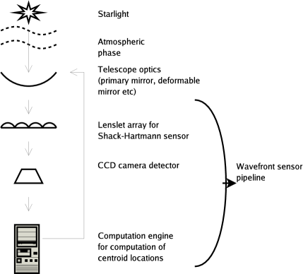
Fig. 1: A schematic diagram of the wavefront sensing process for a typical Shack-Hartmann wavefront sensor.

In a real astronomical AO system, starlight to be used for wavefront sensing will be diverted from the main science beam using, for example, a beam splitter. This diverted beam will then usually be passed through optical elements designed to allow the wavefront shape to be sensed, such as a Shack-Hartmann lenslet array or a pyramid optical element. The beam is then imaged onto a detector, usually a CCD, converted to an electronic form and passed to a processing engine. The processing engine will then use the detected light to determine the shape of the wavefront, for example by employing a centroiding algorithm in the case of a Shack-Hartmann system. The computed shape of the wavefront is then used to shape an optical element, typically a deformable mirror, using a “reconstruction” process. Designs for future AO systems can require this process to be repeated at a rate of 1-5 kHz with tens of thousands of degrees of freedom in the reconstruction process[9]. I now consider only the case of a Shack-Hartmann wavefront sensing system, and an overview of this wavefront sensing process is shown in Fig. 1.

2.A The simulated wavefront sensor pipeline

When simulating the wavefront sensing process, it is necessary to model many physical processes as well as the computational processes (such as the centroid location algorithm) so that the result will be as accurate as possible. When simulating a Shack-Hartmann WFS with the Durham AO simulation platform, I start by computing the atmospheric perturbations that have been introduced into the incident starlight by the time this light has reached the telescope. The wavefront sensing process then computes the following steps:

1. A small phase map (equivalent to a phase tilt) is added to the atmospheric phase in each Shack-Hartmann sub-aperture, so that in the un-aberrated case (with no atmospheric perturbations) the maximum intensity will be placed at the centre of the central four pixels in the sub-aperture once the high light level Shack-Hartmann images are created.

2. A telescope pupil map is used to determine which parts of the telescope aperture are in the optical path.

3. The real and imaginary parts of the atmospheric phase array are computed (assuming an amplitude of unity) by taking the sine and cosine of the phase values.

4. The complex phase values are Fourier transformed using a two dimensional fast Fourier transform (FFT).

5. The high light level (noiseless) image for each sub-aperture is computed by taking the square modulus of the Fourier transform.

6. Any required integration time and re-sampling of the image scale are performed on the high light level images.

7. The light within each sub-aperture is normalized so that the total light within the sub-aperture is equal to that expected from a given source magnitude.

8. A sky-brightness pattern is introduced into the high light level images.

9. Photon shot noise is then added, by replacing the high light level (noiseless) image intensities in each pixel with a Poisson random variable with a mean and variance equal to this intensity.

10. The CCD readout noise is simulated by adding a Gaussian random variable with a mean and variance defined by the level of CCD readout noise to be simulated. The simulated signal is now at the stage where it would be read out from the CCD camera and grabbed into computer memory.

11. Noise sources are subtracted from the signal, for example by applying a threshold value.

12. The centroid location of light within each sub-aperture is then computed.

The centroid locations which are computed by this process are then passed into a software wavefront reconstructor which will typically use a large matrix multiplication operation to determine and update the deformable mirror shape.

2.B Hardware implementation of the wavefront sensing pipeline

When implementing an algorithm in an FPGA, it is important to consider how the algorithm can be parallelised so that the FPGA is used efficiently. I have implemented the WFS pipeline in a way which means that all stages of the pipeline can operate simultaneously on different parts of a dataset. This is demonstrated in Fig. 2. In simple terms, the phase data for one sub-aperture is loaded into the FPGA. The FPGA then begins to compute the 2D Fourier transform of this data while a second dataset is loading into the FPGA. After the Fourier transform has been computed, various noise sources (e.g. photon shot noise) are introduced into the sub-aperture. While this is happening, the second dataset is being Fourier transformed, and the third dataset is being loaded into the FPGA. This highly parallel operation then continues until the results for all sub-apertures have been computed. In reality, the parallelization is even finer as, for example, the Fourier transform will begin while data is still being loaded, and the introduction of photon shot noise will be computed in stages on many different pixel values at the same time.

In a CPU implementation only one stage can happen at a time and so even though the time to compute each stage may be less than with the FPGA implementation, the total computation time will be greater.

2.B.1 The algorithm choice

Many simulation codes (for example propagation codes) contain one part of the simulation where the majority of the computation time is spent computing a simple algorithm. Such simulations are ideal candidates for hardware acceleration because the simple algorithm can easily be placed in hardware, and the resulting performance increase of this part of the simulation also gives a similar performance increase to the simulation as a whole, since this is where the majority of computation time is spent.

However, in an AO simulation, a large amount of computational time is divided between a number of key components since an AO simulation contains many complex algorithms, for example, the reconstruction algorithms, the atmospheric phase screen generation, and various parts of the wavefront sensing pipeline. To give a large overall performance increase for an AO simulation, each of these components would require a performance increase. Amdahl’s law [10] states that the overall system speed is governed by the slowest component. As an example, a simulation may consist of five algorithms, each requiring 20 percent of processor time. If one of these algorithms was then implemented in hardware, which reduced the computational time for this algorithm by a factor of 1000, the overall simulation computational time will only be reduced by about a fifth. It is therefore necessary to reduce the computational time of all five algorithms to achieve an overall performance increase of greater than five times.

This means that most parts of the AO simulation should be implemented in hardware to give a significant performance increase. I have therefore implemented the wavefront sensing algorithms in hardware as a first step, since these algorithms are among the most computationally intensive. Additionally, these algorithms are among the most complicated to place in hardware and so success implementing them gives an idea of the difficulty of implementing the majority of an AO simulation within one or more FPGA.

2.B.2 Data bandwidth considerations

In many computer architectures, data flow – passing data between computational elements – can cause a bottleneck when processes spend significant amounts of time waiting for data. On the Cray XD1 super computer where the hardware wavefront sensing pipeline has been implemented, it is possible to pass data at a theoretical bandwidth of 1.6 GBs^-1 between the FPGA and processor memory in each direction. The highly parallel nature of the FPGA means that many calculations can be computed simultaneously. It is therefore important to ensure that all of these calculations can be fed with necessary data. To do this, I have ensured that data is passed to and from the FPGA only once, with no intermediate results being returned to the CPU memory. This ensures that the FPGA can be fed with new data at all times. If, for example, one intermediate result stage was returned to the CPU memory, operated on by the CPU, and then passed back into the FPGA, the bandwidth available for each data transfer stage would be halved, resulting in an increase in the computation time.

It is therefore essential to program the FPGA so that data flow to and from the host processor memory is minimised.

2.B.3 Algorithms within the wavefront sensing pipeline

Optical phase data (aberrated by the atmospheric turbulence) is currently generated by the CPU, and read by the FPGA at every iteration (time-step) of the simulation. Once computed within the FPGA, the floating point centroid locations are written back to the CPU main memory by the FPGA. I have implemented all of the algorithms described in section 2.A within the hardware implementation of the wavefront sensing pipeline, which is treated as a black box, accepting floating point optical phase data, and returning floating point centroid location values. Internally, data is stored in the most appropriate format chosen to give the required precision while not consuming FPGA resources which are not needed. For example, during the high light level image computation, data is stored in a floating point format with a 22 bit mantissa and a six bit exponent, while during the introduction of photon shot noise, the data is stored as a 23 bit wide fixed point number.

It is important to realise that each stage within the pipeline can operate simultaneously with other stages on different parts of the dataset. In total, about four months of effort was required to implement this algorithm in hardware. The software version on the other hand could be prepared in about a week or so, giving some idea of the differences between software and hardware complexities. The hardware algorithm was implemented in VHDL, a low level hardware description language. Higher level languages are available for hardware programming (such as Handel-C). However, these higher level languages take up much more of the FPGA resources (typically by a factor of two or much more), and can often restrict the maximum clock speed of the FPGA for which the algorithm will give correct results. These factors mean that the wavefront sensing pipeline would not fit into a single FPGA if created using a higher level language. Currently, about 70 percent of the FPGA resources (a Virtex-II Pro V2P50) are used for this pipeline.

2.B.4 Configuration

FPGAs are usually considered to be fixed function devices, performing only one set task (which may be simple or complicated). In the case described here, the fixed function is the WFS algorithms. However, these have been implemented to be configurable:

1. The dimensions of the input optical phase array for each sub-aperture can be selected, up to a maximum of $32\times 32$ values.

2. The size of a two dimensional fast Fourier transform (FFT) (used to create the high light level images from the atmospheric phase) can be chosen from $8\times 8$, $16\times 16$ or $32\times 32$ pixels. If the FFT dimensions are not equal to the optical phase array dimensions, the optical phase is zero-padded inside the FPGA before the FFT is executed.

3. The number of iterations over which the wavefront sensor is to be integrated before being read out is also configurable (up to a maximum of 63 iterations).

4. Pixel re-sampling (binning) can also be configured, with the FFT output being re-sampled to any size from $2\times 2$ pixels up to the size of the FFT (including rectangular arrays).

5. Random number generator seeds can be configured.

6. The shape of the telescope pupil function which is used to determine which sub-apertures are able to collect light can be defined.

7. CCD readout noise parameters can be configured (mean and root-mean-square).

8. A sky background value can be set.

9. A threshold level to be applied to the signal after CCD readout has been simulated can be set.

10. The number of sub-apertures is configurable up to a maximum of $1024\times 1024$ (more sub-apertures can be used when a pupil mask is not required).

11. The magnitude of the guide star can be chosen.

The configurability of this hardware implementation of the wavefront sensing and centroid algorithms means that the benefits of hardware acceleration can be realized for a large range of simulations.

2.C Integration with the AO simulation platform

The hardware accelerated wavefront sensing algorithms have been integrated with the Durham AO simulation platform in such a way that the user needs to specify only whether or not the hardware implementation should be used where possible. There are situations in which this implementation cannot be used (for example when simulating a Pyramid WFS), in which case, a software algorithm is used instead. When an AO simulation is running, it is possible to switch on or off the FPGA acceleration facility using a graphical simulation control interface.

3 Performance improvements

An FPGA should be operated at a clock rate which is dependent on the logic implemented within the FPGA. The synthesis tools used to compile the FPGA code give an indication of what the maximum clock rate should be. Improving the implementation of the logic within the FPGA will often allow a faster clock rate to be used, for example by more efficient pipelining. When the clock rate is set too high, the FPGA will cease to function in the expected way, which can cause data corruption. The FPGA performance is directly dependent on this clock rate.

3.A FPGA clock rate performance

The relative time taken by the software and hardware algorithms determines the performance increase achieved by the hardware implementation. For this purpose, a slightly modified software algorithm was used which computed only the algorithms also computed in the FPGA. Fig. 3 shows the performance increase obtained as a function of FPGA clock speed, and it can be seen that the trend is linear. The dotted line in Fig. 3 shows that at clock speeds above about 170 MHz, the hardware implementation of the algorithm becomes unreliable due to overclocking of the FPGA, sometimes giving incorrect results. Further work on the algorithms within the FPGA to streamline the pipeline would allow the FPGA to give accurate results at these clock rates, though this has not yet been carried out. In the Cray XD1, the FPGAs can be clocked at a maximum rate of 199 MHz, which would give an extra 10 percent increase in performance over the 170 MHz clock rate which currently gives correct results. For the rest of this paper, a clock rate of 170 MHz is assumed unless otherwise stated, so that data integrity is maintained.

3.B Data quantity

The relative performance improvement achieved when using the FPGAs depends partly on the size of the dataset which is accessed by the FPGA. When the dataset is small, the overhead of reading data into the FPGA, and writing the results back to the host CPU memory will be large compared to the time spent computing the results. Therefore, the performance improvement will be small (indeed, there are algorithms in which the FPGA can be slower than the CPU when the dataset is small[11]). The pipeline itself also has some latency, as there is a finite time between the last data entering the pipeline, and the last result leaving the pipeline, of order 700 clock cycles, or 4 $\mu$s (at 170 MHz). Fig. 4 shows the time taken to compute the WFS algorithms when using the hardware and software implementations, as a function of the number of sub-apertures operated on. As can be seen, when using the FPGA implementation, the total computation time is about 20 $\mu$s for small numbers of sub-apertures (up to about $4\times 4$), regardless of the number of sub-apertures used, corresponding to the latency in the pipeline and the latency for memory access. When larger numbers of sub-apertures are used, the computation time is proportional to the number of sub-apertures evaluated.

The time taken for the hardware WFS algorithms to complete can be estimated when the number of sub-apertures is large (greater than about 100), as

$$t=\frac{n_{f}^{2}\times n_{s}\times n_{i}}{f}+t_{l}$$ (1)

where $t$ is the time taken in seconds, $n_{f}$ is the size of the dimensions of the 2D fast Fourier transform (FFT) used to compute the high light level images (8, 16 or 32), $n_{s}$ is the total number of sub-apertures to be evaluated, $n_{i}$ is the number of integrations carried out, $f$ is the clock frequency of the FPGA in Hz and $t_{l}$ is the initial latency of the pipeline, about $20\times 10^{-6}$ s. The massively parallel architecture means that the computation time is simply the computation time of the lowest algorithm (in this case, creating and integrating the high light level images).

When the CPU implementation is used, the computation time is dependent on the number of sub-apertures evaluated. The memory access latency is lower when the calculation is carried out in the CPU, and so the computation time scales closely with the number of sub-apertures to be evaluated even when this is small. The performance increase when using the FPGA is therefore less when smaller numbers of sub-apertures are used, as shown in Fig. 5. A typical current AO system will contain 100 sub-apertures, while future AO systems are planned with over 100, 000 sub-apertures when multiple wavefront sensors are used.

3.C Integrations

When the optical phase data is sampled more than once for each CCD readout simulation, (i.e. the sub-aperture images are integrated before photon shot noise or CCD readout noise is added), it is necessary to pass more data into the FPGA per final centroid value. Since the FPGA computation is limited by the rate at which data is passed in, this will increase the computation time proportionally to the number of integrations. However, the time taken by the software implementation will only be proportional to the number of integrations up to the point at which the integration is carried out. After this, the remainder of the calculation (noise addition, centroid estimation) will be performed only once, meaning the time taken is independent of the number of integrations. Therefore, the total time taken by the software implementation will be less than proportional to the number of integrations, meaning that the relative performance improvement realized by the FPGA will be reduced as shown in Fig. 5.

3.D Sub-aperture size

The computation time of the FPGA implementation of these algorithms is given by Eq. 1. For the software implementation, this is not the case, since an increase in sub-aperture dimensions by a factor of two (i.e. four times as many phase value array elements per sub-aperture) will take less than four times as long to compute, as demonstrated in Fig. 6, due to the different rates at which various algorithms within the pipeline take to complete. This figure shows that performance increase provided by the FPGA is reduced as the sub-aperture size increases. Additionally, whereas for the FPGA implementation, pixel re-sampling does not affect the computation time (due to the fine grain parallel architecture), the CPU implementation run time is effected, taking shorter times to complete when greater binning is used (due to the centroid algorithm then being applied to smaller sub-apertures). The performance increase will therefore be less when the CPU implementation performs relatively faster as shown in Fig. 6. In most AO simulations, small sub-apertures are used with typically $8\times 8$ phase array elements.

4 Future work

The hardware WFS pipeline is useful for a wide range of simulations. The effect of spot elongation when using laser guide stars is not yet considered in this pipeline, and so this could be added, Additionally, taking scintillation effects into account may be necessary for some systems.

Implementing these algorithms within the current FPGAs in the XD1 is unlikely to be possible, due to the finite amount of logic within the FPGAs. However, it is possible to upgrade the XD1 with larger FPGAs, and this would allow these extra algorithms to be implemented within a single FPGA should funds become available.

In a typical software AO simulation at Durham, the WFS algorithms may take about 75 percent of CPU time. By implementing these algorithms in an FPGA, they can be accelerated by over 600 times. The remaining 25 percent of the processor tasks then have full access to the conventional processors. However, this will then only accelerate the AO simulation by a factor of four, not particularly impressive given the acceleration achieved for the WFS algorithms. It is therefore necessary to implement other parts of the simulation within the FPGAs.

The majority of the remaining processor tasks are found within the reconstruction algorithms which map the WFS outputs onto new figures for the deformable mirror optics. It is therefore necessary to implement these algorithms in hardware to accelerate the simulation further. Given the large number of combinations of natural guide stars, laser guide stars and conjugate deformable mirrors, it is not possible to include the reconstruction algorithms as part of the WFS pipeline, but rather, in a separate hardware implementation running within a different FPGA. This will allow for the flexibility and reconfigurability of the AO simulation to be maintained.

The construction of atmospheric turbulence phase screens is also processor intensive, and it is planned to move this algorithm into hardware also. This again will improve the overall performance of the AO simulation.

5 Conclusion

I have described the implementation of a WFS simulation pipeline within reconfigurable logic in the form of FPGAs, and this is the first time that this has been attempted. This has led to a reduction in computation time of over 600 times over the conventional software approach, allowing the simulation run times to be reduced. This work demonstrates the feasibility and benefits of hardware acceleration using FPGAs, and shows that hardware acceleration can greatly improve the performance of calculations, far beyond that achievable by using software based approaches. This has relevance for simulation of a wide range of optical systems. By using a hardware accelerated AO simulation platform, it is possible to model AO systems on extremely large telescopes, which would be otherwise infeasible due to the long computation times.

Fig. 2: A schematic diagram showing the parallelization of the wavefront sensor pipeline within the FPGA. All stages operate simultaneously. Here, NOP means no operation is computed, i.e. the input data is not valid.

Fig. 3: A figure showing the performance increase when using an FPGA instead of a CPU for wavefront sensing pipeline algorithms, as a function of the FPGA clock rate. The dotted line above 170 MHz shows the speeds at which the FPGA algorithm becomes unreliable due to overclocking. Here, the centroid locations of 1024 Shack-Hartmann sub-apertures have been computed at each FPGA clock frequency.

Fig. 4: A figure showing the computation time for the wavefront sensing pipeline in hardware (solid curve) and software (dotted curve) as a function of the number of sub-apertures to be evaluated.

Fig. 5: A figure showing the ratio of CPU to FPGA computation time for the wavefront sensing pipeline as a function of the number of sub-apertures to be evaluated. A typical current AO system will contain 100 sub-apertures, while future AO systems are designed with over 100,000 sub-apertures. The number of image integrations carried out before the CCD readout is simulated is 1 (solid curve), 2 (dotted curve), 4 (dashed curve) and 8 (dot-dashed curve).

Fig. 6: A figure showing the ratio of CPU to FPGA computation time for the wavefront sensing pipeline as a function of the number of pupil phase values per sub-aperture (first number for each bar) and the number of simulated CCD pixels (in each dimension) per sub-aperture (second number for each bar).

1. A schematic diagram of the wavefront sensing process for a typical Shack-Hartmann wavefront sensor.

2. A schematic diagram showing the parallelization of the wavefront sensor pipeline within the FPGA. All stages operate simultaneously. Here, NOP means no operation is computed, i.e. the input data is not valid.

3. A figure showing the performance increase when using an FPGA instead of a CPU for wavefront sensing pipeline algorithms, as a function of the FPGA clock rate. The dotted line above 170 MHz shows the speeds at which the FPGA algorithm becomes unreliable due to overclocking. Here, the centroid locations of 1024 Shack-Hartmann sub-apertures have been computed at each FPGA clock frequency.

4. A figure showing the computation time for the wavefront sensing pipeline in hardware (solid curve) and software (dotted curve) as a function of the number of sub-apertures to be evaluated.

5. A figure showing the ratio of CPU to FPGA computation time for the wavefront sensing pipeline as a function of the number of sub-apertures to be evaluated. A typical current AO system will contain 100 sub-apertures, while future AO systems are designed with over 100,000 sub-apertures. The number of image integrations carried out before the CCD readout is simulated is 1 (solid curve), 2 (dotted curve), 4 (dashed curve) and 8 (dot-dashed curve).

6. A figure showing the ratio of CPU to FPGA computation time for the wavefront sensing pipeline as a function of the number of pupil phase values per sub-aperture (first number for each bar) and the number of simulated CCD pixels (in each dimension) per sub-aperture (second number for each bar).