Medium resolution spectroscopy in $\omega$ Centauri:
abundances of 400 subgiant and turn-off region stars

Medium resolution spectra of more than 400 subgiant and turn-off region stars in $\omega$ Centauri were analysed. The observations were performed at the VLT/Paranal with FORS2/MXU. In order to determine the metallicities of the sample stars, we defined a set of line indices (mostly iron) adjusted to the resolution of our spectra. The indices as determined for $\omega$ Cen were then compared to line indices from stars in the chemically homogeneous globular cluster M55, in addition to standard stars and synthetic spectra. The uncertainties in the derived metallicities are of the order of $\pm 0.2\;{\rm dex}$.

Our study confirms the large variations in iron abundances found on the giant branch in earlier studies ($-2.2<$[Fe/H]$<-0.7\;{\rm dex}$). In addition, we studied the $\alpha$-element and CN/CH abundances. Stars of different metallicity groups not only show distinct ages (Hilker et al. 2004), but also different behaviours in their relative abundances. The $\alpha$ abundances increase smoothly with increasing metallicity resulting in a flat [$\alpha$/Fe] ratio over the whole observed metallicity range. The combined CN+CH abundance increases smoothly with increasing iron abundance. The most metal-rich stars are CN-enriched. In a CN vs. CH plot, though, the individual abundances divide into CN- and CH-rich branches. The large abundance variations observed in our sample of (unevolved) subgiant branch stars most probably have their origin in the pre-enriched material rather than in internal mixing effects. Together with the age spread of the different sub-populations, our findings favour the formation of $\omega$ Centauri within a more massive progenitor.

1 Introduction

In many respects, one of the most extraordinary globular clusters within our Milky Way is $\omega$ Centauri. It is not only the most massive ($3\times 10^{6}\;M_{\odot}$) and with a projected ellipticity of 0.18 one of the most flattened clusters in our galaxy, but it furthermore has a retrograde orbit around the Galactic centre, unlike most other globular clusters.

Table 1: Log of observations

Date	Mask	Position (RA; DEC (J2000))	Exp.time (1400V)	Exp.time (600I)
07/05/2002	ome-1	201.950389   -47.45774	$3\times 900\;{\rm s}$	$2\times 900\;{\rm s}$
08/05/2002	ome-2	201.950367   -47.45791	$3\times 900\;{\rm s}$	$2\times 1200\;{\rm s}$
09/05/2002	ome-3	201.950467   -47.45834	$3\times 900\;{\rm s}$	$3\times 1200\;{\rm s}$
	omw-1	201.499877   -47.47863	$3\times 900\;{\rm s}$	$3\times 1200\;{\rm s}$
10/05/2002	omn-1	201.694769   -47.31202	$3\times 900\;{\rm s}$	$3\times 1200\;{\rm s}$
	oms-1	201.740967   -47.62819	$3\times 900\;{\rm s}$	$3\times 1200\;{\rm s}$
	omss-1	201.739449   -47.72814	$3\times 900\;{\rm s}$	$3\times 900\;{\rm s}$
	M55-1	294.996455   -30.88368	$3\times 600\;{\rm s}$	$3\times 720\;{\rm s}$
11/05/2002	oms-2	201.739332   -47.62879	$3\times 720\;{\rm s}$	$3\times 900\;{\rm s}$
	omn-2	201.694567   -47.31218	$3\times 900\;{\rm s}$	$3\times 960\;{\rm s}$
	omw-2	201.512185   -47.48084	$3\times 720\;{\rm s}$	$3\times 900\;{\rm s}$
12/05/2002	omw-3	201.512222   -47.48080	$2\times 900\;{\rm s}$	$2\times 1200\;{\rm s}$

Although $\omega$ Cen is one of the longest-known globular clusters and has been the subject of countless studies, the history of its investigation is more one of adding enigmatic properties than explaining them. Already Dickens & Woolley (1967) realised the unusual width of the red giant branch (RGB), which was later explained as a spread in metallicity by Cannon & Stobie (1973) and which was spectroscopically confirmed by Freeman & Rodgers (1975). Further spectroscopic analyses revealed significant variations in nearly all element abundances (e.g. Norris & Da Costa 1995; Smith et al. 2000). Especially remarkable is the wide spread in [Fe/H], which covers a range of $-2.0$ to $-0.5\;{\rm dex}$. Both photometric and spectroscopic studies point to multiple stellar populations within $\omega$ Cen, which differ not only in metal abundances but also in their spatial and kinematic properties. The stars on the RGB in $\omega$ Cen can be divided into at least 3 sub-populations. A dominant metal-poor component (peaking at [Fe/H]$\sim-1.7\;{\rm dex}$) contributes about 70% of the stars. This population rotates at a maximum velocity of $V_{\rm rot,max}\sim 8\;{\rm km\>s^{-1}}$ (Merritt et al. 1997). In contrast, the intermediate metallicity population (about 25% of the stars and peaking at [Fe/H]$\sim-1.2\;{\rm dex}$) shows no rotation but rather a concentration towards the cluster centre (Norris et al. 1997). The most metal-rich component comprises about 5% of the stars with metallicities around $-0.6\;{\rm dex}$, and its spatial distribution is off-centre with respect to the more metal-poor populations (Hilker & Richtler 2000). One has to be aware of the changes in nomenclature of these populations over the years. Before the discovery of the most metal-rich population (Lee et al. 1999; Pancino et al. 2000), what are here called metal-poor and intermediate metallicity populations are often referred to as metal-poor and metal-rich.

Recent high-resolution multi-band images reveal that the population puzzle in $\omega$ Cen  is probably even more complicated. Ferraro et al. (2004) discovered, apart from the main subgiant branch (SGB), an additional, narrow, and well-defined SGB in the colour-magnitude diagram (CMD) that seems to be the extension of the very red RGB found by Lee et al. (1999) and Pancino et al. (2000). Also, finer substructures have been identified on the RGB and the main sequence (MS) using HST photometry. Sollima et al. (2005) have revealed the subdivision of the intermediate metallicity population on the RGB into at least 3 discrete populations. Very stunning is also the bifurcation of the MS (e.g. Bedin et al. 2004). The observed fact that the red branch of the MS contains the majority of the stars, which is the opposite of what is observed on the RGB, was at first very puzzling. An unusual Helium enrichment of the intermediate metallicity population now seems to be one of the most favoured explanations for this feature (e.g. Norris 2004; Piotto et al. 2005).

Both spectroscopic and broad and narrow band photometric studies suggest a spread in age (e.g. Lee et al. 1999; Hughes & Wallerstein 2000; Hilker & Richtler 2000; Rey et al. 2004; Hughes et al. 2004). All of these independent measurements reveal a significant age difference between the sub-populations of 2-6 Gyr, correlated in the sense that the younger populations are the more metal-rich ones.

Neither the spread in [Fe/H] nor in age has been observed in any other globular cluster so far. Presumably, the formation history of $\omega$ Centauri differs fundamentally from the ones of the other globular clusters in the Milky Way. There are many different possibilities discussed as conceivable origins of the variations in metal abundances and the observed age spread. One of the most convincing ideas is that $\omega$ Cen has an extragalactic origin, either the isolated nucleus of a formerly disrupted dwarf galaxy or a super-star cluster that has formed in an ancient, violent merger event (e.g. Bekki & Freeman 2003; Fellhauer & Kroupa 2003) .

Most of the spectroscopic studies of $\omega$ Cen have so far been concentrated on the RGB. These gave very accurate metallicity measurements, but only rough age estimates due to the age-insensitivity of the location of RGB stars. With pure photometric investigations, though, it is not possible to achieve accurate metallicity determinations. With 8-meter telescopes, however, it is now possible to obtain spectra of the appropriate resolution of stars near the main sequence turn-off (MSTO) and the SGB, i.e. of stars in a region that is highly sensitive to age.

In this paper, the results of an analysis of more than 400 spectra of stars in this region of the CMD are presented. In particular, the method that has been used for the Fe calibration is described in detail in this paper. Section 2 introduces the observations and summarises the data reduction. The selection of spectra for the final sample is described in Sect. 3. Section 4 deals with the definition of the new line indices used to analyse this spectroscopic data. A detailed description of the dependencies of the measured indices on stellar parameters and the absolute calibration of the Fe indices is given in Sects. 5 and 6. In Sect. 7 we present a qualitative analysis of other lines besides Fe, including Mg, Ca, CH, and CN. A discussion and summary of the results is given in Sect. 8. The age spread of the different sub-populations in $\omega$ Cen was presented in a first paper by Hilker et al. (2004), and an automated analysis of a larger sample of stellar spectra is presented in Willemsen et al. (2005).

2 Observations and data reduction

The instrument used for this project was the Focal Reducer and Low Dispersion Spectrograph 2 (FORS2) attached to the Very Large Telescope (VLT/UT4) at ESO/Paranal (Chile). FORS2 is equipped with a mask exchange unit (MXU) and provides (with the standard resolution collimator) a field of view of $6\hbox{$.\mkern-4.0mu^{\prime}$}8\times 6\hbox{$.\mkern-4.0mu^{\prime}$}8$. The detector system consists of two $4096\times 2048$ MIT CCDs, which were read out in the $2\times 2$ binning mode.

In a preceding study of Hilker & Richtler (2000), a large sample of RGB and MSTO stars in $\omega$ Centauri was analysed using Strömgren photometry. The photometry of this study was used to select the candidate stars for the spectroscopy. Five fields outside the cluster centre were defined in the region covered by the Stömgren photometry. According to their position, the fields were named ‘omn’ (north), ‘ome’ (east), ‘oms’ (south), ‘omw’ (west) and ‘omss’ (south-south). Figure 1 shows the position of these fields with respect to the Strömgren data. For this project, we primarily selected stars with magnitudes in the range 17$<V<$18 mag and colours of 0.25$<(b-y)<$0.55 mag, and those without direct neighbours to allow a proper sky subtraction. In total, 11 slit masks have been defined.

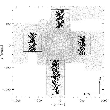
Figure 1: This plot shows in grey the region of $\omega$ Cen that is covered by Strömgren photometry (Hilker & Richtler 2000). All stars with a $V$ magnitude brighter than 19.0 mag and a photometric error less than 0.1 mag have been plotted. The squared areas indicate the 5 defined fields in which the candidate stars for the spectroscopy have been selected (bold dots).

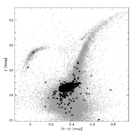
Figure 2: Position of the programme stars (filled triangles) in the Strömgren CMD of $\omega$ Cen (Hilker & Richtler 2000). The open triangles are those objects identified as non cluster members by their radial velocities. All objects crossed out have been rejected due to the velocity or other selection criteria, such as quality of the spectrum and close neighbouring stars (see Sect. 3).

A slit mask contained 50 to 60 slits with fixed width of 1^′′ and a length of 4-8^′′. Occasionally, one slit covered more than one object. About 40 stars were observed through more than one slit mask. Those objects were used to verify the consistency between the observations of the different nights/masks.

The observations were performed between May 7, 2002 and May 12, 2002. In total, spectra of $\sim$620 selected objects were observed. The seeing was between $0\hbox{$.\!\!^{\prime\prime}$}6$ and $1\hbox{$.\!\!^{\prime\prime}$}0$ in all nights. Each slit mask was observed through two different grisms with the ESO denotations 1400V+18 and 600I+25 (second order). In the $2\times 2$ binning mode the first grism has a dispersion of $0.62\;{\rm{\AA}\;pix^{-1}}$ in the spectral range 4560 to $5860\;{\rm\AA}$. The latter covers the range 3690 to $4888\;{\rm\AA}$ with a dispersion of $0.58\;{\rm{\AA}\;pix^{-1}}$. The individual wavelength coverage depends on the position of the slit on the mask. Lines located in the overlapping wavelength range could be used to check the consistency between the measurements of the two different grisms. Each mask was observed two or three times with typical total exposure times of 45 min for the 1400V grism and 60 min for the 600I grism (see Table 1). Moreover, for each field/mask, calibration exposures such as bias, flat-field, and lamp spectra were obtained.

During the same observing run, one mask for stars was observed near the MSTO/SGB of the globular cluster M55. This chemically homogeneous cluster with a well-known metallicity of [Fe/H]=$-1.8\;{\rm dex}$ (e.g. Zinn 1985; Caldwell & Dickens 1988; Richter et al. 1999) serves as a comparison and calibration object. Furthermore, spectra of 17 standard stars with known abundances (mostly from Cayrel de Strobel et al. 2001) were obtained with the same grism in the long slit mode.

The data reduction was performed with the IRAF-packages ONEDSPEC and TWODSPEC. The mask-exposures were bias corrected, cleaned for cosmic-rays (using BCLEAN from the STARLINK package), and combined. The combined spectral images were response-calibrated using dome-flat spectra. No absolute flux calibration was performed. Next, the individual stellar spectra were extracted. In most cases, object and sky could be extracted from the same slit. For about 90 stars the sky was taken from another closeby slit and subtracted with the SKYTWEAK task. The lamp exposures were extracted in the same way as the science exposures.

For the wavelength calibration, we used 9-15 lines of the elements He, Ne, Hg, and Cd for the 1400V grism. In case of the blue grism (600I, 2nd order), 7-12 He, Hg, and Cd lines were used for the calibration. The overall uncertainty of the wavelength calibration was found to be $0.01\;{\rm\AA}$ (rms). For further analyses, all spectra were binned to a spectral scale of $1\;{\rm{\AA}\;pix^{-1}}$ in the ranges 3520 - $5100\;{\rm\AA}$, for the blue, and 4340 - $6120\;{\rm\AA}$ for the red grism. The final spectral resolution (FWHM) for narrow lines is $\sim 2.5\;{\rm\AA}$. The signal-to-noise ratio (S/N) varied between 30 and 100 per pixel depending on the grism, wavelength range, and luminosity of the star. The data for M55 and the standard stars were reduced to wavelength-calibrated spectra in the same way.

Figure 3: This figure illustrates the different strengths of the metal lines in the continuum-normalised spectra of three different stars. From top to bottom a metal-rich, an intermediate, and a metal-poor star are shown. Note that the three stars have roughly the same temperature so that the differences in line strengths are due purely to abundance variations.

3 Grid of observed spectra

The spectra sample included stars with different luminosities and at different positions on the slit mask. In order to obtain a more homogeneous set, we therefore applied several selection criteria.

First, we classified the spectra based on their overall quality. We sorted out those spectra with errors resulting from bad tracing of the spectrum, either due to its position at the border of the slit (star not fully in the slit) or due to its faintness. Also, spectra of stars that are located closer than 2^′′ to a bright neighbouring star in dispersion direction were left out, since it is possible that their spectral contributions overlap. Second, we rejected all but the exposure with the highest S/N of those stars that had been observed multiple times through different slit masks. In total, 508 stars (of originally 662 individual spectra) passed these quality checks.

We went on to select the stars based on their observed radial velocity. These were determined using the IRAF tasks RVIDLINES and FXCOR. Since $\omega$ Cen has a heliocentric velocity of $232.3\;{\rm km\;s^{-1}}$ (Harris 1996), foreground stars could easily be identified by their much lower radial velocities. We selected all those stars with observed radial velocities in the range 150 to $350\;{\rm km\>s^{-1}}$. This wide range was chosen to account for possible systematic effects in the velocity determination that have not been corrected for (e.g. slight mismatches of the arc-lamp and science exposures during day and night observations). The radial velocity selection resulted in a sample of 483 member stars with good quality.

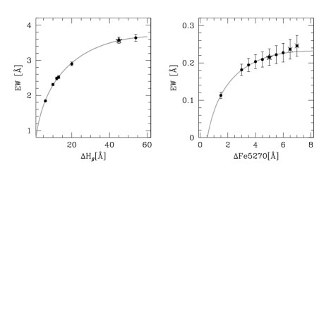
Figure 4: Effects of the variation in the width of the index bandpasses on the measured EW for two exemplary lines (H_β and Fe5270). The curves are second-order fits to the data points. Excluded data points are crossed out.

The selected widths of the bandpasses are marked with asterisks.

The final step was to select only SGB/MSTO-region stars from the member sample. We included only those stars with magnitudes of $16.8<V_{0}<18.2\;{\rm mag}$ and colours of $0.4<(B-V)_{0}<0.8\;{\rm mag}$. Our final sample contains 429 stars.

4 Measurement of line indices

For the spectroscopic analysis we defined 42 line indices that include 25 of the strongest iron lines, hydrogen lines, 3 calcium and 3 magnesium lines, and the CH-band at $4300\;{\rm\AA}$. The lines were identified and selected by means of the “Bonner Spektralatlas” (Seitter 1970, 1975) and the online database NIST.

For each of these lines a central bandpass region and two flanking continuum regions on either side were defined with typical bandwidths of $5-20\;{\rm\AA}$. We chose the widths of the central bands in such a way that only the line to be measured was included. This approach was problematic for the strong Balmer and calcium lines, though. These lines have extended wings in which one can find lines of other elements. In case of the weaker Fe lines it was very important to minimise the effects of neighbouring lines, since even weak neighbouring lines can have a considerable influence on the measured equivalent width (EW). Figure 4 illustrates the effect of varying the width of the central line bandpass on the measured line indices using the example of the ${\rm H_{\beta}}$ and the Fe5270 line. With larger width of the central line bandpass ($\Delta\rm H_{\beta}$ and $\Delta\rm Fe5270$), the EW first increases very rapidly and only marginally after the whole line is covered by the bandpass. With the further increase of the bandwidth the influence of included neighbouring lines can be seen, especially for the weaker Fe5270 line. We selected the bandwidth large enough to cover the whole line but as well small enough to prevent major effects by neighbouring lines. In the case of very close lines of the same element the central bandpass was extended to cover all of them. These indices were labelled with “B_” (=band).

Following the specifications in the Lick system, the EW of an index was determined by the flux difference between the pseudo-continuum and the spectrum in the range of the bandpass (e.g. Worthey et al. 1994). The pseudo-continuum is defined as a line drawn between the midpoints of the two continuum bandpasses. There were 6 line indices defined in the overlapping wavelength region of the two grisms. Those indices were measured in both the red and blue spectra individually, and the indices are correspondingly labelled ‘r’ and ‘b’ . Figure 5 shows the location of some of the defined line indices, and Tables 2 and 3 summarise all indices.

For the automatic measurement of the line indices we used a program (gonzo.prl) provided by Thomas H. Puzia. This algorithm measures line indices of abundance features on ASCII files for any kind of spectra. The overall errors are estimated based on the Poisson noise of the spectra, on the errors in the velocity determination, and by the uncertainties of the sky spectrum.

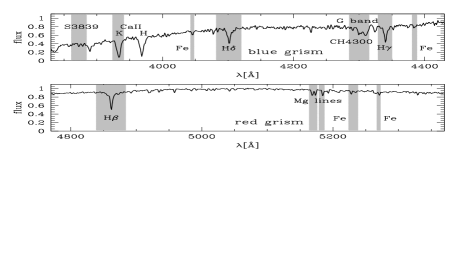
Figure 5: The blue and red part of a spectrum of a typical SGB star of $\omega$ Cen is shown. The maximum count rate was normalised to unity. The shaded regions mark most of the bandpasses that were used to measure iron and Balmer line indices as well as CN, CH and $\alpha$ indices.

Table 2: Definition for line indices in the blue grism

Index	central bandpass		blue continuum		red continuum
	l. limit	u. limit	l. limit	u. limit	l. limit	u. limit
CN_Fe	3853.5	3875.0	3847.0	3853.0	3909.0	3923.0
CaII_K	3924.0	3942.0	3909.0	3917.0	3988.0	3995.0
CaII_H	3954.0	3987.0	3909.0	3917.0	3988.0	3995.0
Mn4032	4027.5	4036.5	4018.5	4027.0	4037.0	4042.5
Fe4045	4043.0	4048.0	4037.0	4042.0	4049.0	4061.0
Fe_B01	4061.5	4080.0	4049.0	4061.0	4115.5	4128.5
Hδ	4082.0	4120.0	4049.0	4061.0	4147.0	4166.0
Fe4132	4129.0	4136.5	4116.0	4128.5	4137.0	4141.0
Fe4143	4141.5	4146.0	4137.0	4141.0	4146.5	4166.0
Fe_B02	4184.0	4206.0	4146.5	4166.0	4206.5	4213.5
Fe4215	4213.5	4218.0	4206.5	4213.5	4230.5	4245.0
Fe_Ca	4223.5	4229.5	4206.5	4213.5	4230.5	4245.0
G4300	4282.0	4318.0	4239.0	4269.0	4357.0	4370.0
CH	4322.0	4328.0	4239.0	4269.0	4357.0	4370.0
Hγ	4329.0	4350.0	4239.0	4269.0	4364.0	4371.0
Fe4376	4373.0	4380.0	4357.0	4370.0	4409.0	4413.0
Fe4383	4381.0	4388.0	4355.0	4370.0	4409.0	4413.0
Ti4395	4391.5	4397.0	4355.0	4370.0	4409.0	4413.0
Fe4405	4402.5	4409.0	4355.0	4370.0	4409.0	4413.0
Ca4455	4452.0	4457.0	4432.0	4451.0	4458.0	4473.0
bTi4534	4530.0	4536.5	4504.0	4524.0	4537.0	4545.0
bFe4549	4546.0	4552.0	4537.0	4545.0	4552.0	4570.0
bHβ	4839.0	4884.0	4815.0	4829.0	4895.0	4905.0
bFe4920	4915.5	4922.0	4901.5	4915.0	4941.5	4952.0
bFe4957	4954.0	4960.0	4942.0	4952.0	4961.0	4980.0
bFe_B03	5003.5	5021.0	4992.0	5003.0	5021.0	5038.5

Table 3: Definition for line indices in the red grism

Index	central bandpass		blue continuum		red continuum
	l. limit	u. limit	l. limit	u. limit	l. limit	u. limit
rTi4534	4530.0	4536.5	4504.0	4524.0	4537.0	4545.0
rFe4549	4546.0	4552.0	4537.0	4545.0	4552.0	4570.0
rHβ	4839.0	4884.0	4815.0	4829.0	4895.0	4905.0
rFe4920	4915.5	4922.0	4901.5	4915.0	4941.5	4952.0
rFe4957	4954.0	4960.0	4942.0	4952.0	4961.0	4980.0
rFe_B03	5003.5	5021.0	4992.0	5003.0	5021.0	5038.5
Fe5041	5039.0	5044.0	5021.0	5039.0	5054.0	5064.0
Fe5139	5136.5	5141.5	5116.0	5136.0	5144.0	5161.0
Mg_1+2	5164.0	5177.0	5144.0	5161.0	5210.0	5223.5
Mg5183	5179.0	5187.0	5144.0	5161.0	5210.0	5223.5
Fe_B04	5224.0	5238.0	5210.0	5223.5	5239.0	5259.0
Fe5270	5267.0	5272.5	5240.0	5259.0	5286.0	5311.0
Fe5328	5322.5	5331.0	5299.5	5316.0	5351.0	5365.5
Fe5371	5368.0	5373.5	5351.0	5365.5	5375.0	5394.0
Fe5397	5394.0	5400.0	5375.0	5394.0	5410.0	5422.0
Fe5405	5402.0	5408.0	5375.0	5394.0	5410.0	5422.0
Fe_B05	5426.0	5437.0	5410.0	5422.0	5459.0	5471.0
Fe5446	5442.0	5450.0	5410.0	5422.0	5459.0	5471.0
Fe5455	5453.0	5458.0	5410.0	5422.0	5459.0	5471.0
Mg5528	5523.0	5533.0	5512.0	5522.0	5535.0	5546.0
Na_D1	5888.0	5893.0	5863.0	5877.0	5900.0	5910.0
Na_D2	5894.0	5898.5	5863.0	5877.0	5900.0	5910.0

We performed tests to check the self-consistency of the measurements and to estimate the errors. As mentioned in Sect. 2 the covered spectral ranges of the two grisms slightly overlap. In Fig. 6 we compare the measured equivalent widths for 2 of the 6 lines (Ti4534 and Fe4549) located in this region. Although the scatter for the Ti4634 is quite large and there might be some overestimation of the line strength of Fe4549 in the red spectrum, we consider the agreement acceptable, in particular when taking into account that the lines are very weak and located close to the edge of the spectra. The tracing of the spectrum in these regions was difficult during the data reduction. Bad tracing leads to a misdefinition of the pseudo continuum and therefore to mismeasurements of the line strengths.

Another check on the accuracy of the measurements is provided by stars that were observed through more than one slit-mask. For those objects the defined line-indices were measured twice. Accordingly, one would expect identical values for the EW. As an example, Fig. 7 shows the comparison of the indices H_δ, H_γ, Fe5270, and Fe_B04 that were measured in different spectra of identical stars. In these graphs only data with a fractional error of less than 50% of the index value are shown. For all indices one sees good consistency within the errors.

Figure 6: Comparison of indices measured in both grisms (Ti4534 and Fe4549).

In order to calculate a more accurate indicator for hydrogen and iron, we averaged several individual line indices to a single-line index for a given element. For hydrogen, we combined 2 of the 3 prominent Balmer lines:

$$\rm{\langle H\rangle=(H_{\gamma}+H_{\delta})/2}.$$ (1)

During the analysis we found that index ${\rm H_{\beta}}$ showed strong discrepancies as compared to ${\rm H_{\gamma}}$ and ${\rm H_{\delta}}$. ${\rm H_{\beta}}$ is the strongest of these three Balmer lines and has very extended wings at these temperatures and surface gravities. It is very likely that the influence of lines in those wings and non-linearities effects cause the observed deviance. We therefore excluded ${\rm H_{\beta}}$ from the combined H-index.

In order to get an average iron index, 6 of the strongest iron lines and one magnesium line of similar strength were combined. Before averaging the 7 indices, they were weighted in such a way that their line strengths are of the same order. In other words, the weaker indices were multiplied by larger weighting factors than the stronger indices. The weighting factors were defined in the following way: the line strength versus $\langle{\rm H}\rangle$ distribution of each individual index was fitted by a linear least-square fit, i.e. Fe4045 $=a\cdot\langle{\rm H}\rangle+b$. The reciprocal of the fit value at $\langle{\rm H}\rangle$ = 3 defines the weighting factor $w$, i.e. $w_{\rm Fe4045}=1/(3a+b)$. With this definition, the combined iron index scatters around 1 at $\langle{\rm H}\rangle$ = 3 (see e.g. Fig. 11). The formula for the combined iron index showing the weighting factors of the individual indices is:

$$\rm{\langle Fe\rangle} = \rm{(4.13\cdot Fe4045+2.91\cdot Fe\_Ca+3.67\cdot Fe4383}$$ (2)

$$\rm{+3.42\cdot Mg5183+4.08\cdot Fe\_B04+4.04\cdot Fe5270}$$

$$\rm{+4.67\cdot Fe5328)/7}.$$

This iron index was used in combination with the combined hydrogen index (see above) for the subsequent analysis.

Figure 7: Comparison of indices (H_δ, H_γ, Fe5270, and Fe_B04) measured in different spectra of the same star. The 1:1 correlation is indicated by the dashed line. All line indices affirm the very good consistency between the different nights/masks.

5 Analysis of the line indices

5.1 Luminosity, surface gravity, and temperature effects

Besides the element abundance, the strength of the iron lines depends on other stellar parameters. The most important ones here were the effects of effective temperature ($T_{\rm eff}$) (or correspondingly the colour of the star) and the surface gravity (log $g$) of the star.

In order to analyse the impact of these parameters on the line strengths, we used synthetic spectra provided by Bailer-Jones (2000). We adjusted their step size ($0.5\;{\rm{\AA}\;pix^{-1}}$) and resolution ($\sim 1\;{\rm\AA}$) to the observed data ($1\;{\rm{\AA}\;pix^{-1}}$ and $\sim 2-2.5\;{\rm\AA}$). Additionally, we scaled the synthetic counts to the order of magnitude of the observational data. We used spectra of different metallicities ($-2.0,-1.5,-1.0$ and $-0.5\;{\rm dex}$), effective temperatures ($5000-7000\;{\rm K}$), and surface gravities (range $3.2$ to $4.6$ dex). On the synthetic spectra, we then measured the line indices introduced above in the same way as for the stellar spectra of $\omega$ Cen .

As an example, the dependence of the strongest iron line Fe5270 on $T_{\rm eff}$ and log $g$ is shown in Fig. 8. One can see that the temperature is a major influence on the line index at those parameter values ($3.2<$ log $g$ $<4.1$ dex and $5400<$ $T_{\rm eff}$ $<6000$ K). To correct for the effects of temperature, we used the combined Balmer index $\langle{\rm H}\rangle$, which shows a strong correlation with the $(B-V)_{0}$ colour (see Fig. 9). The scatter in the $\langle{\rm H}\rangle$ -$(B-V)_{0}$- diagram is mainly caused by an additional, but weak, dependence on metallicity and log $g$.

Figure 8: Effects of temperature and surface gravity. The upper panel shows the measured Fe5270 index as a function of the effective temperature for four different iron abundances ([Fe/H]), with constant $log\hskip 2.84526pt$g$\ =3.5$. Due to the temperature effect, the measured EW increases with decreasing effective temperature for constant [Fe/H]. In the lower panel the Fe5270 index is plotted versus log $g$ in case of four different [Fe/H] and a constant temperature $\hbox{$T_{\rm eff}$}\ =6000\;{\rm K}$.

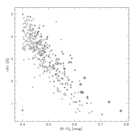
Figure 9: This figure shows the coherency between mean Balmer index $\langle{\rm H}\rangle$ and the $(B-V)_{0}$ colour for the $\omega$ Cen data. $\langle{\rm H}\rangle$ mainly depends on temperature, as demonstrated by the relatively small scatter in this diagram, and therefore can be used as a temperature indicator. The scatter in this diagram is due to small metallicity effects on $\langle{\rm H}\rangle$ and $(B-V)$: the light grey dots indicate stars with iron abundances between $-2.0$ and $-1.4\;{\rm dex}$; the grey triangles are for those with $-1.4<$[Fe/H]$<-1.0\;{\rm dex}$, and the dark asterisks are for stars with $-1.0<$[Fe/H]$<-0.5\;{\rm dex}$.

5.2 Comparison with M55 spectra

One possibility for deriving absolute metallicities is comparing the line strengths of the stars in $\omega$ Cen with those in M55. This globular cluster has a similar distance to the Sun ($d_{M55}=5.4\;{\rm kpc}$ and $d_{\omega Cen}=5.2\;{\rm kpc}$; Harris 1996); i.e. the MSTO stars have luminosities comparable to those of $\omega$ Cen  ($V_{\rm MSTO}\sim 17.5\;{\rm mag}$), and thus their spectra are of the same quality in terms of S/N. After clearing the M55 sample of non-members (by radial velocities) and selecting stars with $0.35<(B-V)_{0}<0.68\;{\rm mag}$ and $17.1<V_{0}<17.8\;{\rm mag}$ we measured the defined line indices on the remaining 36 spectra. As for $\omega$ Cen, we calculated a combined Fe and H index. The upper panels of Fig. 10 show the $\langle{\rm Fe}\rangle$-$\langle{\rm H}\rangle$-diagrams for both $\omega$ Cen and M55. As the M55 stars have a well-known iron abundance of [Fe/H]$=-1.8\;{\rm dex}$, their average position in the $\langle{\rm Fe}\rangle$-$\langle{\rm H}\rangle$-diagram can serve as reference in the $\omega$ Cen plot.

Figure 10 shows that $\omega$ Cen has a much larger variation in iron abundances than M55. Furthermore, one can see that most of the stars have higher abundances than [Fe/H]$=-1.8\;{\rm dex}$. This result is in qualitative agreement with former results for RGB stars (e.g. Norris & Da Costa 1995; Suntzeff & Kraft 1996).

Although the $\langle{\rm Fe}\rangle$-$\langle{\rm H}\rangle$-relation of M55 stars cannot be used for an absolute calibration of the most metal-rich stars in $\omega$ Cen, it is very useful to estimate the accuracy of the index measurements. The analysis of the scatter of the M55 stars around the fit (upper right panel) reveals a standard deviation of $\sigma_{M55}({\rm Fe})\sim 0.10\;{\rm\AA}$ (see Fig. 10 lower panel). The EW is proportional to the number of absorbing atoms (for non-saturated lines, which can be assumed for the weak Fe lines), i.e. EW${}_{\rm Fe}\sim N_{\rm Fe}$ and [Fe/H]$\sim{\rm log}N_{\rm Fe}$. By defining an upper and lower error in EW ((${\rm EW}+\Delta{\rm EW}$) and (${\rm EW}-\Delta{\rm EW}$)) we estimated the internal error in [Fe/H] to be $0.12\;{\rm dex}$.

In the lower left panel in Fig. 10 we plotted the scatter around the fit curve of the $\omega$ Cen data (upper panel of Fig. 10). The standard deviation for this fit is $\sigma_{\omega\;Cen}({\rm Fe})\sim 0.22\;{\rm\AA}$, significantly larger than that for M55. This a clear indication of an intrinsic broad scatter in [Fe/H] in the region of the MSTO and SGB.

5.3 Comparison with standard stars

In addition to the observations of M55, we obtained spectra of stars with known stellar parameters. These are referred to as ‘standard’ stars in the following. The spectra of these stars have higher S/N values than the globular cluster spectra (typically $\sim 80-150$ at $4500\;{\rm\AA}$ and $\sim 180-220$ at $5100\;{\rm\AA}$). From the sample of 17 observed standard stars, we selected 11 stars with spectral types of SGB/MSTO region stars. Table 4 summarises their properties. On these spectra we again measured the line indices and calculated the average iron and hydrogen indicators $\langle{\rm Fe}\rangle$ and $\langle{\rm H}\rangle$ as defined in Sect. 4.

For more clarity, we divided the standard stars into four groups according to the [Fe/H] values given by the literature. All stars with Fe abundances higher than $-0.95\;{\rm dex}$ are classified as most metal-rich, followed by stars with metallicities in the range $-1.3<$[Fe/H]$<-0.95\;{\rm dex}$ and $-1.8<$[Fe/H]$<-1.3\;{\rm dex}$. Stars with [Fe/H]$<-1.8\;{\rm dex}$ are termed as ‘metal-poor’.

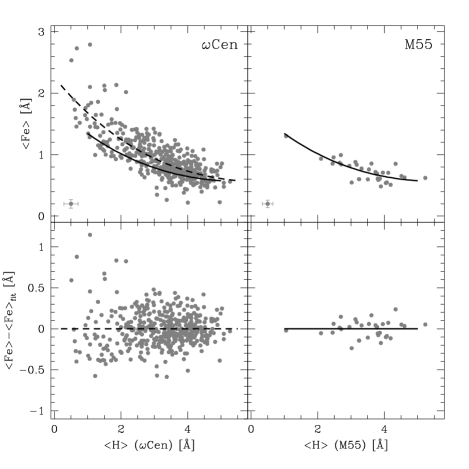
Figure 10: The upper two panels show the $\langle{\rm Fe}\rangle$- $\langle{\rm H}\rangle$- diagrams of 410 MSTO/SGB stars in $\omega$ Cen (left) and 36 M55 stars (right). The $\omega$ Cen data points show a much larger scatter in the $\langle{\rm Fe}\rangle$ index. The solid line is an exponential fit to the M55 data points and therefore marks the position of stars with [Fe/H]$=-1.8\;{\rm dex}$ in both diagrams. The dashed line in the left panel is an exponential fit to the $\omega$ Cen data points. In the lower left corner the average error is shown. The two lower figures show the scatter of the $\omega$ Cen and M55 data points around the fit curves. The scatter in $\omega$ Cen is much larger than in M55 and can only be explained by the wide intrinsic metallicity spread.

In Fig. 11, we plot the $\langle{\rm Fe}\rangle$-$\langle{\rm H}\rangle$ diagram for $\omega$ Cen, together with the data points of the standard stars. The positions of the different groups of standard stars mark the relation between $\langle{\rm H}\rangle$, $\langle{\rm Fe}\rangle$, and [Fe/H]. The metal-poor standards form a lower limit for the distribution of $\omega$ Cen stars, whereas the most metal-rich standards form an upper limit. Most stars of $\omega$ Cen are associated with an Fe abundance between $-2.0$ and $-1.3\;{\rm dex}$.

5.4 Comparison with synthetic spectra

Another independent calibration method is the use of synthetic spectra (see Sect. 5.1). By measuring the same line indices on these spectra and by calculating $\langle{\rm Fe}\rangle$ and $\langle{\rm H}\rangle$ we were able to derive synthetic iso-metallicity curves in the $\langle{\rm Fe}\rangle$-$\langle{\rm H}\rangle$-diagram. Only synthetic spectra with $T_{\rm eff}$ and log $g$ values that are consistent with MSTO/SGB stars (adopted from the isochrone set by Kim et al. (2002)) were considered. In this way, the iso-metallicity curves are implicitly corrected for the log $g$ effect of MSTO/SGB stars (see Fig. 8).

Table 4: General properties of the standard stars used for the metallicity calibration. The values are taken from the SIMBAD database (http://simbad.u-strasbg.fr/Simbad)

Name	$V$	$B-V$	Type	log $g$	[Fe/H]	Hβ
	[mag]	[mag]		[dex]	[dex]	[mag]
BD-032525	9.67	0.48	F3	3.60	$-$1.90	2.59
BD-052678	11.92	0.59	F7	4.43	$-$1.89	2.59
BD-084501	10.59	0.59	F8	4.00	$-$1.40	2.59
BD-133442	10.37	0.32	F	4.20	$-$2.72	–
HD089499	8.68	0.74	F8	3.00	$-$2.23	2.54
HD097916	9.17	0.38	F5V	4.20	$-$0.92	2.64
HD179626	9.14	0.53	F7V	3.70	$-$1.26	2.59
HD192718	8.41	0.54	F8	4.00	$-$0.74	–
HD193901	8.67	0.53	F7V	4.58	$-$1.03	2.57
HD196892	8.23	0.50	F6V	4.14	$-$1.00	2.59
HD205650	9.00	0.59	F8V	4.38	$-$1.03	–

6 Absolute calibration of the abundances

The absolute calibration of iron abundances was done by using all calibrators introduced above. The distribution of the standard stars, the M55 fit curve, and the iso-metallicity curves of the synthetic spectra are shown in Fig. 11. The metallicity positions of all calibrators are consistent with each other, the $\omega$ Cen data points are plotted for reference.

In order to derive the absolute [Fe/H] abundances for the $\omega$ Cen stars from their $\langle{\rm H}\rangle$ and $\langle{\rm Fe}\rangle$, we established an analytical relation of the form [Fe/H]=f($\langle{\rm Fe}\rangle$, $\langle{\rm H}\rangle$). A polynomial fit of 4th order in both coordinates was used with full cross-terms. The determined metallicities were analysed in our previous paper (Hilker et al. 2004). As our sample is strongly biased by the selection of the target stars, our metallicity distribution is not representative for $\omega$ Cen; hence we do not show the biased metallicity distribution here.

The total errors in [Fe/H] were derived from the errors in the measurements of the individual line indices and the error of the derived relation between $\langle{\rm H}\rangle$, $\langle{\rm Fe}\rangle$ and [Fe/H]. The former are based on the Poisson noise of the spectra, the errors in the velocity determination and on the uncertainties on the sky spectrum, whereas the latter include the uncertainties of the polynomial fit.

In order to estimate the error resulting from the calibration method, we compared the [Fe/H] literature values with those calculated by our established analytical relation for the standard stars, the M55 data, and the synthetic data points. Figure 12 shows the difference between the [Fe/H] values as derived from our calibration versus the literature values. For the case of M55, we plot five values with different $\langle{\rm H}\rangle$. The scatter of the calibrators around the calibration relation is $\sigma_{\rm calib}({\rm Fe})\sim 0.04\;{\rm\AA}$.

The total errors in [Fe/H], $\delta$[Fe/H], were found to be of the order of $0.1-0.3\;{\rm dex}$. As the most luminous stars ($\approx 16.5\;{\rm mag}$) in our sample provide the spectra with the highest S/N ratios, the measured indices on those spectra have the smallest errors. The mean relative error in [Fe/H] for stars between V=16.6 and 17.0 mag is $\delta$[Fe/H]/[Fe/H]$=5.1\%$, whereas for fainter stars ($18.0<V<18.4$) this error is $12.5\%$. That temperature has a major effect on the strength of the Fe lines (Sect. 5.1) is reflected in the relative errors of [Fe/H]. Figure 13 shows the relation of the relative error in [Fe/H] with $\langle{\rm H}\rangle$ i.e. temperature. For lower $\langle{\rm H}\rangle$ (lower $T_{\rm eff}$), the relative errors are smallest. In other words, for a given [Fe/H] the observed iron lines are stronger the lower the effective temperature $T_{\rm eff}$ (in the temperature regime considered by us). Consequently, the total errors in [Fe/H] are mainly influenced by the luminosity and temperature of the individual stars (see Fig. 13).

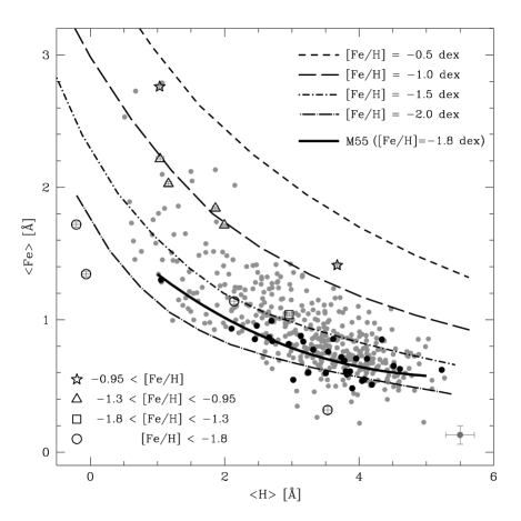
Figure 11: This plot shows the distribution of 410 MSTO/SGB stars in $\omega$ Cen (grey dots) in the $\langle{\rm Fe}\rangle$-$\langle{\rm H}\rangle$-diagram with respect to all three independent calibrators. The positions of the 11 standard stars are plotted for four metallicity ranges as indicated in the lower left. The bold curve is the fit of the M55 datapoints as derived in Sect. 5.2. The dashed lines are the iso-metallicity curves as calculated from the synthetic spectra. These lines are constructed in such a way that they account for the log $g$ effect on the SGB where log $g$ decreases steadily from 4.1 to 3.5 with increasing $\langle{\rm H}\rangle$. All independent calibration methods are consistent with each other and allow for an assignment of absolute iron abundances. The average error bar is given in the lower right.

Figure 12: Scatter of the calibrated iron abundances versus their literature values. The standard stars are marked as bold dots, the synthetic data points as open symbols. Five sample points out of the M55 fit curve are given as asterisks.

Figure 13: The dependency of relative error in [Fe/H] on V, $\langle{\rm H}\rangle$ (i.g. $T_{\rm eff}$), and [Fe/H]. For brighter and cooler stars the determined [Fe/H] values have the smallest relative errors.

7 Relative abundances of light elements in the different sub-populations

In addition to Fe, we also measured indices of the Ca and Mg lines and of the CN and CH bands. The calcium index $\langle{\rm Ca}\rangle$ is just the strength of the Ca K line. The magnesium index $\langle{\rm Mg}\rangle$ is the average of the Mg indices Mg_1+2 and Mg5183 (see Table 3). For a qualitative analysis of CN and CH abundances, we measured the modified S3839 and CH4300 indices used by Harbeck et al. (2003), which are defined as

$${\rm S3839=-2.5\;log\frac{F_{3861-3884}}{F_{3894-3910}}},$$ (3)

$${\rm CH4300=-2.5\;log\frac{F_{4285-4315}}{0.5F_{4240-4280}+0.5F_{4390-4460}}}$$ (4)

where F are the fluxes in the different bandpass regions. For comparison, we again measured the same indices in the M55 stars, expecting to show no strong variations in the light-element abundances.

In the following we describe the correction of the measured indices for effects of temperature and compare the relative abundances of the thus-weighted indices for the different sub-populations in $\omega$ Cen. An absolute calibration of $\alpha$ and C, N abundances is foreseen for a future study.

7.1 Correction of temperature effects

We restricted our analysis of the light elements to the cooler/redder part of the subgiant branch, in the magnitude and colour range $16.9<V_{0}<17.8$ and $(B-V)_{0}>0.44$. Since even this colour-selected set of stars shows a considerable range in temperature, we need to apply a correction that eliminates the effects of temperature on the strength of the absorption lines.

As a temperature indicator, we used the combined hydrogen index $\langle{\rm H}\rangle$ (see Sect. 5.1). Figure 14 shows the dependence of the different element indices on $\langle{\rm H}\rangle$. As expected, the line strengths for the different elements/molecules increase on average with decreasing $\langle{\rm H}\rangle$ (decreasing temperature). For CN, however, there is no such strong dependence since the strength of the CN line at 3839 Å only weakly depends on temperature (see e.g. Jaschek & Jaschek 1995).

In order to correct for the effects of temperature, we fitted a second order polynomial to the lower boundary of each index in Fig. 14. The ‘temperature corrected’ index is then calculated from the vertical distance $\langle{\rm index}\rangle-$fit, and the resulting value (‘$\delta$’) is further scaled by the median value for a given index. In the following, these corrected and scaled indices are denoted by, e.g., $\overline{\delta\langle{\rm Mg}\rangle}$.

Due to the stronger line indices at lower temperatures, the abundance variations can be analysed best in the regime of low $\langle{\rm H}\rangle$ values. For the subsequent analyses, we therefore selected SGB stars between $1<$$\langle{\rm H}\rangle$$<2.2$. The exact selection boundaries are shown in Fig. 14. Their inclinations are motivated by lines of equal temperatures as derived from the synthetic spectra in Fig. 11. The selected temperature range is about 5300-6100 K. Furthermore, we restricted the sample to the colour range $0.50<(B-V)_{0}<0.68$ mag. All these selection criteria ensure a minimisation of the temperature effects while maximising the signal of intrinsic abundance variations between the individual SGB stars. It should be further noted that the restriction to stars on the subgiant branch mostly excludes possible effects of atmospheric mixing as would be expected to occur in giant branch stars (see e.g. Thorén et al. 2004).

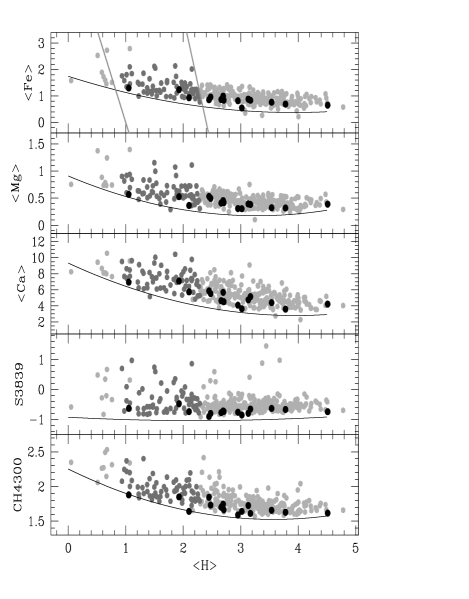
Figure 14: Different line indices versus the hydrogen index $\langle{\rm H}\rangle$. From top to bottom: iron indicator $\langle{\rm Fe}\rangle$, magnesium index $\langle{\rm Mg}\rangle$, calcium index $\langle{\rm Ca}\rangle$, CN-band indicator S3839, and CH-band index CH4300. The black dots are stars from the comparison cluster M55. Dark grey dots indicate those stars that were selected for further analyses. Besides the boundaries in the upper panel, the selection criteria are a colour range of 0.5$<(B-V)_{0}<$0.68 mag.

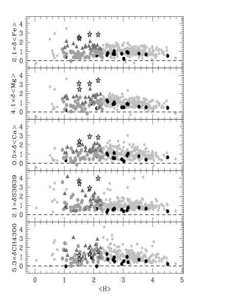
Figure 15: Normalised and ‘temperature-corrected’ line indices versus the hydrogen index $\langle{\rm H}\rangle$. The black dots are stars from M55. Light dots are all the data points for $\omega$ Cen. The darker symbols mark the selected stars (see Fig. 14) in different metallicity bins: dots indicate stars with iron abundances between $-2.0$ and $-1.4\;{\rm dex}$; the grey triangles are for those with $-1.4<$[Fe/H]$<-1.0\;{\rm dex}$, and the dark asterisks are for stars with $-1.0<$[Fe/H]$<-0.5\;{\rm dex}$.

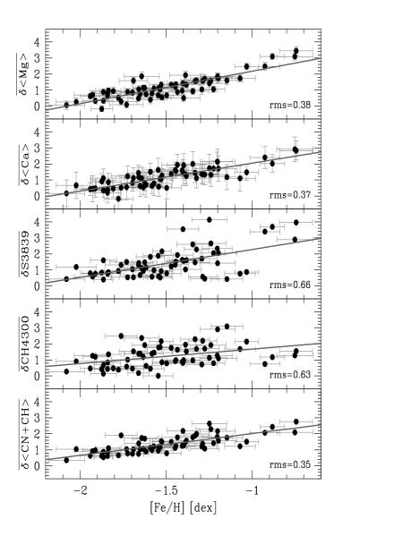
Figure 16: Normalised and ‘temperature-corrected’ line indices versus iron abundance [Fe/H]. Only stars in the selected regions of Figs. 14 and 15 are considered. The lines are fits to the data points with the rms indicated. Clearly, the scatter of the combined index $\overline{\delta\langle{\rm CN+CH}\rangle}$ is significantly smaller than those of the individual indices alone.

7.2 The dependencies of light elements on iron abundances

The normalised and temperature-corrected indices as a function of the metallicity [Fe/H] are shown in Fig. 16. It can be seen that for the five indices analysed ($\overline{\delta\langle{\rm Mg}\rangle}$, $\overline{\delta\langle{\rm Ca}\rangle}$, $\overline{\delta CH4300}$, $\overline{\delta S3839}$, and $\overline{\delta\langle{\rm CN+CH}\rangle}$) there is a correlation in the sense that the line strengths increase for increasing metallicities. Given that we only consider stars on the SGB with (on average) the same luminosity and since we only make use of temperature corrected line indices, we conclude that the observed dependencies reflect the chemical enrichment history of these stars in $\omega$ Cen. Interestingly, the most metal-rich stars ([Fe/H] $\geq$ $-$1 dex) do not show a significantly larger $\overline{\delta CH4300}$ as compared to e.g. stars with [Fe/H] $\sim$ $-$1.5 dex. For $\overline{\delta S3839}$, however, we find significantly higher values for the metal-rich population (but note the two CN-rich stars at [Fe/H] $\sim$ $-$1.4 dex). In particular, there is an anticorrelation among $\overline{\delta S3839}$ and $\overline{\delta CH4300}$ for the most metal-rich stars. This could most readily be explained by the enrichment of CNO-processed material (with increased N and decreased C). However, that only the most metal-rich stars seem to show this anticorrelation is puzzling. A careful examination of the location of these stars in the colour-magnitude diagram shows that the most metal-rich stars are not the reddest ones. Moreover, these stars have rather intermediate luminosities (as compared to the overall sample of stars) at these colours. This indicates that the observed anticorrelation is not due to (not corrected for) temperature and/or luminosity effects or that these stars occupy a special region in the colour-magnitude diagram. Instead, it could be that the enrichment history for these stars was indeed very different from that of the earlier populations. The scatter as measured by the rms of the best-fitting line is much larger for $\overline{\delta S3839}$ and $\overline{\delta CH4300}$ than for the $\alpha$ elements Mg and Ca (as measured by $\overline{\delta\langle{\rm Mg}\rangle}$ and $\overline{\delta\langle{\rm Ca}\rangle}$). Under the assumption that $\overline{\delta S3839}$ mostly depends on N while $\overline{\delta CH4300}$ is a measure of C abundance, we conclude that there is indeed a wide range of C and N abundances, similar to what was found for RGB stars by Norris & Da Costa (1995).

It should be also noted that the average index $(\delta S3839+\delta CH4300)/2$ ($=$ $\overline{\delta\langle{\rm CN+CH}\rangle}$ in Fig. 16) shows a strong correlation with increasing [Fe/H] and a significantly smaller scatter as compared to the individual indices $\overline{\delta S3839}$ and $\overline{\delta CH4300}$. This was also observed by Hilker & Richtler (2000), albeit for RGB stars. The fact that the CN/CH anticorrelation is not only visible on the RGB but is also detected for almost unevolved stars on the SGB strongly suggests that mixing effects cannot be the dominant cause of the increase of C and N for higher metallicities. Instead, this shows that the enrichment of subsequent stellar populations by the light elements followed that of the iron peak elements.

7.3 Line strengths of $\alpha$ elements

The $\alpha$-elements are important tracers for the enrichment by SN II events. Figure 17 shows the temperature-corrected and scaled Mg over Fe and Ca over Fe absorption-line strengths as a function of [Fe/H]. For both elements, we find that the ratio remains almost constant over the whole metallicity range (up to $\sim$ $-$0.8 dex). The flatness of the $\alpha$ elements, here for SGB-stars, has also been found by Norris & Da Costa (1995) for RGB-stars in the same metallicity range. This is interpreted as a signature for an enrichment dominated by SN II events. Pancino et al. (2002) detected indications for SN Ia enrichment only at very high metallicity ($>-$0.8 dex), which our stars hardly reach. Moreover, it should be noted that the number of stars at higher metallicities is rather low, thus lowering the statistical significance of our analysis.

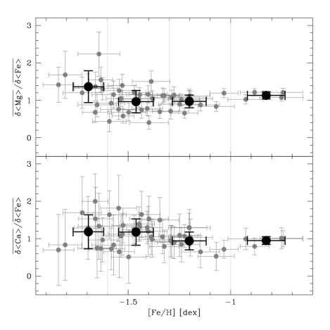
Figure 17: Ratio of magnesium (upper panel) and calcium (lower panel) to the iron index versus iron abundance [Fe/H] for selected stars (see text). The bold data points are averages for the given metallicity bins (vertical lines).

In general, it appears that the spread in [$\alpha$/Fe] is wider for lower metallicities. This is possibly not only due to the larger number of low-metallicity stars in our sample but rather because of the overall higher uncertainty in the measurements for shallower absorption lines at overall lower metallicities (as indicated by the larger error bars). Nevertheless, we cannot exclude the possibility that some fraction of this scatter is due to the chemical enrichment process in $\omega$ Cen. The scatter would then reflect the enrichment by stochastical SN II events during the early star formation phase.

7.4 CN/CH line strengths

The dependence of the temperature-corrected, scaled indices for CN ($\overline{\delta S3839}$) on CH ($\overline{\delta CH4300}$) is shown in Fig. 18. In general, we find that there is a large scatter in the CH and CN abundances of stars in $\omega$ Cen, as compared to e.g. M 55. Indeed, while most of the stars in M 55 are confined to a small region in the CH vs. CN diagram, the stars in $\omega$ Cen show a large scatter towards higher CH or higher CN abundances.

Such a spread was also found by Stanford et al. (2004) in their analysis of 450 MS and MSTO stars in $\omega$ Cen. In their comparison with other galactic globular clusters, they showed that this behaviour can be seen neither for any other globular cluster in their sample nor for close Galactic disk and halo stars. The only other globular cluster showing such a bimodal distribution of CN and CH abundances, but to a much smaller degree, is 47 Tuc. Stanford et al. (2004) argue that the reason for the unique CN/CH spread in $\omega$ Cen might be the much larger iron abundance of its stars .

Figure 18 includes plots of $\overline{\delta CH4300}$ vs. $\overline{\delta S3839}$ for different ranges of the metallicity [Fe/H]. It can be seen that the low-metallicity stars show a wide spread in CH, but there are only few CN-rich stars. For high metallicities, however, there are only stars with moderate CH but with high CN-band strengths; i.e. these stars are possibly enriched in N and depleted in C. The large scatter towards higher CH or CN abundances in the $\overline{\delta S3839}$ vs. $\overline{\delta CH4300}$ diagram (see also Stanford et al. 2004) could be explained by a prolonged enrichment history in a galactic environment. In a scenario where $\omega$ Cen was the nucleus of a gas-rich dwarf galaxy, the intermediate metallicity sub-populations of $\omega$ Cen would have been created from the enriched material of this underlying galactic disk population.

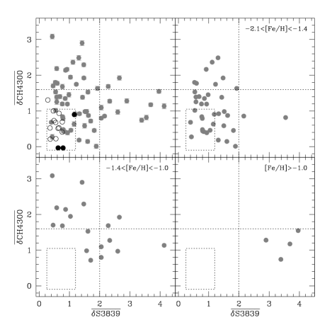
Figure 18: Normalised and ‘temperature-corrected’ CN versus CH index. In the upper right panel all selected stars (see Fig. 14 and 15) are shown, together with the stars in M55 that are confined to a small area (dotted box). Filled dots show stars in M55 in the selected temperature range, while open symbols show all examined stars in M55. The other panels show the CN versus CH index for three different metallicity bins as indicated. The horizontal and vertical lines divide the group of stars into CH-rich and CN-rich populations.

8 Summary and conclusions

The spectra of 429 stars near the SGB/MSTO region of the globular cluster $\omega$ Cen were analysed in the wavelength range $3500$ to $6200\;{\rm\AA}$. The equivalent widths of newly-defined line indices were measured. Absorption lines in the overlapping wavelength regions of the two grisms, as well as repeatedly observed stars, were used to prove the consistency and to estimate the uncertainties of our measurements. In order to calculate an index with high sensitivity to Fe, we combined seven individual line indices to an average iron indicator $\langle{\rm Fe}\rangle$. Furthermore, we defined a mean Balmer index $\langle{\rm H}\rangle$ that served as a temperature indicator.

The same indices were measured on spectra of the chemically homogeneous cluster M55, in addition to standard stars and synthetic spectra. These indices were used to estimate the dependence of $\langle{\rm Fe}\rangle$ on temperature and surface gravity and to establish an analytical function [Fe/H]=f($\langle{\rm Fe}\rangle$, $\langle{\rm H}\rangle$). The error in the absolute iron abundance calibration is of the order $\pm$ 0.1 to 0.3 dex.

Furthermore, we measured Mg, Ca, CN, and CH indices for the $\omega$ Cen and M55 spectra to study the abundance variations in the different populations. The [$\alpha$/Fe] ratio is fairly flat over a wide range of metallicities, indicating a prolonged enrichment by massive (M $>$ 10 $M_{\odot}$) stars. Moreover, we showed that the strong CN and CH variations (which had been found on the RGB before, see e.g. Hilker & Richtler 2000) are also found among the stars in the MSTO/SBG region, i.e. these variations most possibly have a primordial origin so are not due to mixing effects. While the combined CN+CH abundance smoothly increases with metallicity, the enrichment in C and N is anti-correlated. The most metal-rich stars show an extreme enrichment in the CN-bands, whereas metal-poor stars are scattered to high CH abundances, probably pointing to a fast C enrichment by more massive AGB stars.

The abundance patterns of the stars in $\omega$ Cen are uncommon among the globular cluster population of our Milky Way. This refers not only to the iron abundance but also to the lighter element abundances. The strong abundance variations of the light elements indicate that $\omega$ Cen experienced a very complex enrichment history and that the progenitor of this object must have been a far more massive object that was able to retain ejecta by its subsequent generations of stars. Whether this enrichment was due to homogeneous or episodic star formation must be left to a more detailed analysis that includes information on s- and r-process elements, which would allow more accurate models of the star formation rate and the initial stellar mass distributions to be derived.

Over the past years, many studies have revealed more and more peculiarities of $\omega$ Cen. Deep photometry enabled a more detailed inquiry of the bifurcation of the MS found by Anderson (1997), which can most probably be explained as an He overabundance of the intermediate metallicity population (Norris 2004 and Piotto et al. 2005), thus complicating the interpretation of the chemical-enrichment history of $\omega$ Cen. Up to now there no self-consistent models exist for the origin of $\omega$ Cen, but most studies suggest a complex formation scenario in order to explain the unusual observed properties of this globular cluster. Our study provides further evidence of a scenario in which $\omega$ Cen was embedded in a formerly larger galactic entity that was captured and disrupted by the Milky Way.

In our previous study (Hilker et al. 2004), we show that $\omega$ Cen has experienced an extended star-formation history over a period of at least 3 Gyr. In combination with the abundance patterns presented in this study, the combined information shares many similarities with what is found for nearby dwarf galaxies that are known to have experienced rather complex star-formation processes (e.g. Shetrone et al. 2003; Tolstoy et al. 2002; Lanfranchi & Matteucci 2003).

In general, star formation histories vary from dwarf to dwarf galaxy. Both a continuous star formation and bursts seem to be common among the Local Group dSphs (Grebel 1999). Furthermore, Harbeck et al. (2001) have found significant population gradients in Local Group dSphs in the sense that the more metal-rich and younger sub-populations are concentrated towards the galaxies’ centres. This is also observed among the stars in $\omega$ Cen  (e.g. Norris et al. 1996), thus in agreement with a galactic origin of this cluster.

In a forthcoming paper a much more detailed analysis of a larger sample of stars in $\omega$ Cen is foreseen. Combined with precise photometry from HST, the larger spectroscopic data set will be used to shed more light on the enrichment history of this cluster. In particular, we will take the suggested variations in He abundances into account, which can have a non-negligible effect on the derived ages for the different stellar populations.