The Star Formation History of the Universe

Abstract

Strong constraints on the cosmic star formation history (SFH) have recently been established using ultraviolet and far-infrared measurements, refining the results of numerous measurements over the past decade. Taken together, the most recent and robust data indicate a compellingly consistent picture of the SFH out to redshift $z\approx 6$, with especially tight constraints for $z<1$. There have also been a number of dedicated efforts to measure or constrain the SFH at $z\approx 6$ and beyond. It is also possible to constrain the normalisation of the SFH using a combination of electron antineutrino flux limits from Super-Kamiokande measurements and supernova rate density measurements. This review presents the latest compilation of SFH measurements, and summarises the corresponding evolution for stellar and metal mass densities, and supernova rate densities. The constraints on the normalisation of the cosmic SFH, arising from the combination of the supernova rate measurements and the measurement limit on the supernova electron antineutrino flux, are also discussed.

School of Physics, University of Sydney, NSW 2006, Australia

1. Introduction

In the past few years measurement of the evolution of galaxy luminosity functions at a broad range of wavelengths has rapidly matured. One consequence of this has been the refinement in our understanding of how the space density of the galaxy star formation rate (SFR) evolves (Lilly et al. 1996; Madau et al. 1996). In particular the cosmic star formation history (SFH) is now quite tightly constrained (to within $\approx 30-50\%$) up to redshifts of $z\approx 1$. Combined with measurements at higher redshifts the SFH is well determined (within a factor of about 3 at $z\mathrel{\hbox{\hbox to0.0pt{\hbox{\lower 4.0pt\hbox{$\sim$}}\hss}\hbox{$>$}}}1$) up to $z\approx 6$ (e.g., Hopkins 2004).

Additional results from the Super-Kamiokande (SK) particle detector provide a strong limit on the electron antineutrino ($\overline{\nu}_{e}$) flux, 1.2 cm^-2 s^-1 (for $E_{\nu}>19.3\,$MeV), originating from supernova type II events associated with the SFH (Malek et al. 2003). This limit on the diffuse supernova neutrino background (DSNB) constrains the normalisation of the SFH (Fukugita & Kawasaki 2003; Strigari et al. 2005). An exploration of quantities predicted from the SFH, the stellar and metal mass density evolution, and supernova (SN) rate evolution, provides further insight into the allowable normalisation of the SFH (Strigari et al. 2005). This series of interconnected physical properties of galaxies and SNe provides an emerging opportunity for determining the level of the SFH normalisation, and the SFH measurements particularly for $z\mathrel{\hbox{\hbox to0.0pt{\hbox{\lower 4.0pt\hbox{$\sim$}}\hss}\hbox{$<$}}}1$ now have the precision to allow this exploration of their accuracy. Constraining the normalisation of the SFH will support a range of quantitative analyses of galaxy evolution, including the mass-dependence of the SFH (e.g., Papovich et al. 2006; Juneau et al. 2005; Heavens et al. 2004), and the reasons underlying the decline in the SFH to low redshifts (e.g., Bell et al. 2005).

The analysis of the constraints on the SFH normalisation are detailed in Hopkins & Beacom (2006), and here the main arguments are summarised. Since optical SNII can be hidden from observations by dust obscuration, the present SNII rate density measurements may merely be lower limits, and serve as a lower bound on the allowable SFH normalisation. In contrast, since neutrinos are unaffected by dust, the DSNB provides an absolute upper limit on the true SNII rate. We assume $H_{0}=70\,$km s^-1 Mpc^-1, $\Omega_{M}=0.3$, $\Omega_{\Lambda}=0.7$.

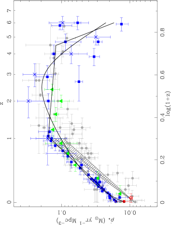
Figure 1.: Evolution of SFR density with redshift (scaled assuming the SalA IMF). Circles are from the compilation of Hopkins (2004). The hatched region is the $24\,\mu$m SFH from Le Floc’h et al. (2005). Triangles are $24\,\mu$m data from Pérez-González et al. (2005). The open star at $z=0.05$ is based on 1.4 GHz data from Mauch (2005). The filled circle at $z=0.01$ is the H$\alpha$ estimate from Hanish et al. (2006). Squares are UV data from Baldry et al. (2005); Wolf et al. (2003); Arnouts et al. (2005); Bouwens et al. (2003a, b, 2005a); Bunker et al. (2004); Ouchi et al. (2004). Crosses are the UDF estimates from Thompson et al. (2006).

2. The Data

The compilation of Hopkins (2004) was taken as the starting point for this analysis, and uses their “common” obscuration correction where necessary. Additional measurements are indicated in Figure 1, and are detailed in Hopkins & Beacom (2006).

2.1. Dust Obscuration Corrections

To implement effective obscuration corrections for the UV measurements at $z\mathrel{\hbox{\hbox to0.0pt{\hbox{\lower 4.0pt\hbox{$\sim$}}\hss}\hbox{$<$}}}1$, we take advantage of the well-established FIR SFR densities up to $z=1$ from Le Floc’h et al. (2005). The UV data at $z\leq 1$ are “obscuration corrected” by adding the FIR SFR density from Le Floc’h et al. (2005) to each point. As shown by Bell (2003a) for individual systems, this technique results in $\dot{\rho}_{*}$ estimates consistent with the obscuration corrected H$\alpha$ measurements. This result is consistent with the interpretation of Takeuchi et al. (2005) that about half the SFR density in the local universe is obscured by dust, increasing to about 80% by $z\approx 1$. For obscuration corrections to the UV data between $1<z<3$ we rely on the fact that the FIR measurements of Pérez-González et al. (2005) are quite flat in this domain, as well as being highly consistent with those of Le Floc’h et al. (2005) at $z<1$, and add the constant SFR density corresponding to that of Le Floc’h et al. (2005) at $z=1$. This is also consistent with the recent measurements of obscuration corrections for UV luminosities at $z\approx 2$ by Erb et al. (2006), who find a typical correction factor of $\approx 4.5$. At higher redshifts we apply a “common” obscuration correction to the UV data as detailed in Hopkins (2004).

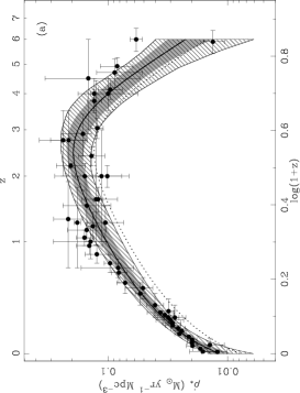
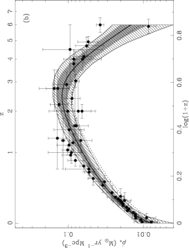
Figure 2.: SFH data used in the parametric fitting. (a) Assumes SalA IMF. (b) Assumes BG IMF. The shape of the fits is determined from the SFH data alone, and a scaling factor is fit to ensure consistency with the SK $\overline{\nu}_{e}$ limit Solid lines assume a $\overline{\nu}_{e}$ temperature of $T=4\,$MeV or $T=6\,$MeV, and dotted $T=8\,$MeV. The grey shaded and hatched regions are the $1\,\sigma$ and $3\,\sigma$ confidence regions around the $T=4\,$MeV fits respectively.

2.2. IMF Assumptions

While uncertainties in SFR calibration act to increase the scatter in the SFH, and uncertainties in dust obscuration can raise it to greater or lesser degrees, the choice of IMF is the only assumption that can systematically decrease the SFH normalisation. A modified Salpeter (1955) IMF, with a turnover below $1\,M_{\odot}$, remains a reasonable model (e.g., Baldry & Glazebrook 2003), and other currently favoured IMFs include those of Kroupa (2001) and Baldry & Glazebrook (2003). The factor to convert SFH measurements from a traditional Salpeter (1955) IMF to the IMF of Baldry & Glazebrook (2003, hereafter BG IMF) is $0.50$ ($-0.305\,$dex). To convert to the modified Salpeter A IMF (Baldry & Glazebrook 2003, hereafter SalA IMF) is a factor of 0.77 ($-0.114\,$dex). The Kroupa (2001) IMF and the modified Salpeter B IMF (Baldry & Glazebrook 2003, hereafter SalB IMF) have scale factors intermediate between these choices. With these two extreme IMF choices we expect to provide bounds encompassing the result from choosing any reasonable IMF in our subsequent analysis.

3. SFH Fitting

To derive a $\overline{\nu}_{e}$ flux from the DSNB for comparison with the limits from SK, we first fit a functional form to the SFH. We use the parametric form of Cole et al. (2001): $\dot{\rho}_{*}=(a+bz)h/(1+(z/c)^{d})$, here with $h=0.7$. The individual $\dot{\rho}_{*}$ measurements chosen to constrain this fit are also important since the resulting fit will obviously vary depending on the data used. The details of the data selected are given in Hopkins & Beacom (2006), and the results shown in Figure 2. The final parametric fitting is a simple $\chi^{2}$ fit to the 58 selected $\dot{\rho}_{*}$ measurements spanning $0\leq z\mathrel{\hbox{\hbox to0.0pt{\hbox{\lower 4.0pt\hbox{$\sim$}}\hss}\hbox{$<$}}}6$.

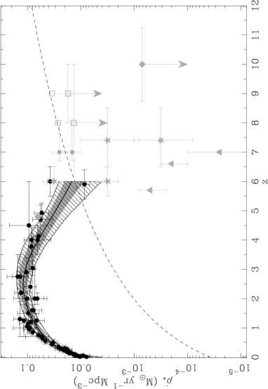
Figure 3.: SFH measurements emphasising recent $z\mathrel{\hbox{\hbox to0.0pt{\hbox{\lower 4.0pt\hbox{$\sim$}}\hss}\hbox{$>$}}}6$ estimates (assuming the SalA IMF). The filled circles and grey shaded and hatched regions are as in the previous Figure (note the different axes scales). The dashed line corresponds to the level of (unobscured) SFH required for reionisation (Madau et al. 1999). Triangles: Ly$\alpha$ emitters (Iye et al. 2006); Stars: LBGs in GOODS (Bouwens & Illingworth 2006); Filled squares: LBGs in GOODS (Mannucci et al. 2006); Diamond: LBGs in the HUDF (Bouwens et al. 2005b); Hexagon: LBGs (A. Verma et al., 2006, this proceedings); Open squares: lensed LBGs (Richard et al. 2006). In all cases where the same symbols appear at the same redshift, the upper values correspond to the maximum expected SFH after integration over the full luminosity function.

3.1. UV Data at High Redshift

As a brief aside, it is worth discussing star formation at $z\mathrel{\hbox{\hbox to0.0pt{\hbox{\lower 4.0pt\hbox{$\sim$}}\hss}\hbox{$>$}}}6$, as there are now a large number of estimates in the literature spanning this range. These primarily use the photometric dropout technique to select Lyman break galaxies (LBGs), often using relatively small, very deep fields (including the Great Observatories Origins Deep Survey, GOODS, and the Hubble Ultra Deep Field, HUDF). Measurements of Ly$\alpha$ emission typically show SFH measurements significantly lower than those from LBGs. It is not clear whether the same populations are being probed here, or the full extent of the selection biases that may be present.

The $z\mathrel{\hbox{\hbox to0.0pt{\hbox{\lower 4.0pt\hbox{$\sim$}}\hss}\hbox{$>$}}}6$ SFH contributes a negligible fraction to the integrated SFH that produces the DSNB, and is neglected in the subsequent analysis. It is, however, of great significance to the epoch of reionisation, and star formation may in fact play the dominant role here. Figure 3 shows the measurements of the $z\mathrel{\hbox{\hbox to0.0pt{\hbox{\lower 4.0pt\hbox{$\sim$}}\hss}\hbox{$>$}}}6$ SFH, based on rest-frame UV luminosities not corrected for obscuration effects. The dashed line in this Figure is the level of SFR density required for reionisation at a given redshift (Madau et al. 1999) assuming $f_{\rm esc}=1$, appropriate for unobscured UV emission, and a clumping factor $C=30$.

Figure 4.: The $\overline{\nu}_{e}$ energy spectra predicted for the various SFH fits and temperature assumptions. The solid and dashed curves are the SalA IMF and BG IMF respectively. The $T=4\,$MeV and $T=6\,$MeV curves are consistent with the SK $\overline{\nu}_{e}$ limit. The $T=8\,$MeV curves are inconsistent with the $\overline{\nu}_{e}$ limit, and indicate the shape of the $\overline{\nu}_{e}$ spectrum derived by assuming the parametric form for the SFH corresponding to our best fit ($T=4\,$MeV), and setting the $\overline{\nu}_{e}$ temperature to the higher value. The thin vertical line marks $E=19.3\,$MeV, above which the $\overline{\nu}_{e}$ contribute to the SK limit.

Although the issue of dust obscuration at high redshift is still highly uncertain, some data is beginning to be obtained. In addition to the $E(B-V)$ estimates from Ouchi et al. (2004), intriguing evidence for significant obscuration ($A_{V}\approx 1\,$mag) at $z=6.56$ has recently been established through Spitzer observations of a lensed Lyman $\alpha$ (Ly$\alpha$) emitting source (Chary et al. 2005). This implies that the first epoch of star formation in this source must have occurred around $z\approx 20$. This is also supported by spectroscopic Ly$\alpha$ emission measurements of LBGs at $z\approx 5$ (Ando et al. 2005), suggesting that the bright LBGs (at least) lie in dusty, chemically evolved systems at this redshift. One promising suggestion here is that the cosmic SFH beyond $z\approx 6$ can be probed through galaxy archeology, i.e., by determining the star formation histories of the $z\approx 6$ galaxy population (see also R.-R. Chary 2006, this proceedings).

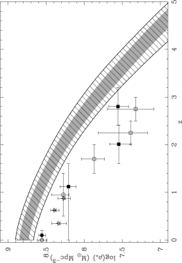
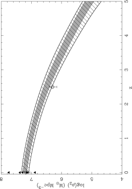
Figure 5.: Left: Evolution of stellar mass density buildup inferred from the SFH. Right: Evolution of metal mass density buildup inferred from the SFH. Refer to Hopkins & Beacom (2006) for references to the measurements shown in both panels. The grey shaded and hatched regions come from the $1\,\sigma$ and $3\,\sigma$ confidence regions around the $T=4\,$MeV fits to the SFH respectively. The SalA IMF is assumed in all cases.

3.2. The Diffuse Supernova Neutrino Background

The DSNB derived from the cosmic SFH is calculated as follows. The $\dot{\rho}_{*}(z)$ is first converted to a type II supernova rate history, $\dot{\rho}_{\rm SNII}(z)$. For the IMFs explored here $\dot{\rho}_{\rm SNII}(z)=(0.0132/M_{\odot})\,\dot{\rho}_{*}(z)$ for the BG IMF and $\dot{\rho}_{\rm SNII}(z)=(0.00915/M_{\odot})\,\dot{\rho}_{*}(z)$ for the SalA IMF. The predicted differential neutrino flux (per unit energy) is then calculated by integrating $\dot{\rho}_{\rm SNII}(z)$ multiplied by the $\overline{\nu}_{e}$ emission per supernova, appropriately redshifted, over cosmic time (see Hopkins & Beacom 2006, for details). Finally, this energy spectrum is integrated above 19.3 MeV to establish the $\overline{\nu}_{e}$ flux for comparison with the SK limit of 1.2 cm^-2 s^-1 (Malek et al. 2003). We explore the implication of assuming a temperature of $T\approx 4\,$MeV, 6 MeV, or 8 MeV. Given the $\overline{\nu}_{e}$ flux for each temperature, we simply scale the best fitting SFH to ensure the SK limit is not violated. The best fit SFHs independent of the $\overline{\nu}_{e}$ limit are identical to the fits constrained by a $\overline{\nu}_{e}$ temperature of $T=4\,$MeV. As found and discussed in Yüksel et al. (2005), our results favour effective temperatures at the lower end of the predicted range.

In addition to the Cole et al. (2001) parameterisation, we also explored a piecewise linear SFH model in $\log(1+z)-\log(\dot{\rho}_{*})$ space, in order to test the possibility that the Cole et al. (2001) parametric model could be biasing the shape of the resulting SFH fit in some way. In this model we allow the following six parameters to vary: The $z=0$ intercept, the slopes of three linear segments and the two redshift values at which the slopes change.

4. Results and Discussion

Figure 1 shows the current SFH data compilation (assuming the SalA IMF) emphasising the additional data used in this analysis compared to the compilation of Hopkins (2004). The best fitting Cole et al. (2001) form for this IMF is also shown as is the best-fitting piecewise linear fit. Figure 2 shows the data used in the fitting and the best fits assuming three temperature values for the $\overline{\nu}_{e}$ population for each IMF assumed. The fitting parameters are tabulated in Hopkins & Beacom (2006).

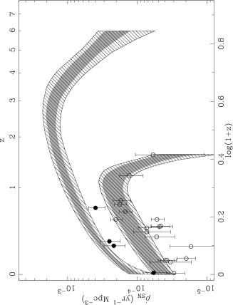
Figure 6.: Evolution of SN rates inferred from the SFH. The upper curves correspond to the predictions for $\dot{\rho}_{\rm SNII}$, and the lower for $\dot{\rho}_{\rm SNIa}$, assuming a delay time $t_{Ia}=3\,$Gyr. See Hopkins & Beacom (2006) for references to the measurements shown.

For both assumed IMFs it can clearly be seen that the assumption of $T=8\,$MeV, when the SFH is required to be consistent with the $\overline{\nu}_{e}$ flux limit, is inconsistent with the SFH measurements. Also for both IMFs, the best fitting SFH assuming $T=6\,$MeV is identical to that assuming $T=4\,$MeV. This can be understood by considering the SalA IMF, for example, with the higher SFH normalisation, but which also has a lower conversion factor between $\dot{\rho}_{*}$ and $\dot{\rho}_{\rm SNII}$, causing the predicted $\overline{\nu}_{e}$ flux to be within the SK limit even with the assumption of the slightly higher neutrino temperature. For both IMF assumptions we determine the $1\,\sigma$ (grey-shaded) and $3\,\sigma$ (hatched) confidence regions around the best fitting SFH (corresponding to $T=4$ or $6\,$MeV). Subsequent Figures reproduce these confidence regions in the predictions for stellar and metal mass density evolution ($\rho_{*}(z)$ and $\rho_{Z}(z)$, respectively) and SN rate evolution ($\dot{\rho}_{\rm SN}(z)$). The shape of the $\overline{\nu}_{e}$ energy spectra corresponding to the various fits for the different IMF and temperature assumptions are shown in Figure 4 (see also Beacom & Strigari 2006).

4.1. Stellar and Metal Mass Densities

Figure 5 shows the evolution of the stellar mass density, $\rho_{*}(z)$, (a far more extensive compilation of data appears in Figure 4 of Fardal et al. 2006), and the metal mass density, $\rho_{Z}(z)$, as inferred from the SFH (Pei & Fall 1995; Madau et al. 1996). The predictions from the best fitting SFH are also shown. For the evolution of $\rho_{*}(z)$ we need to know the fraction of the stellar mass recycled into the interstellar medium as stellar winds or SN ejecta, $R$, corresponding to each IMF (Cole et al. 2001; Madau et al. 1998). We find $R=0.40$ for the SalA IMF, and $R=0.56$ for the BG IMF. The stellar mass inferred is then a fraction $(1-R)$ of the time integral of the SFH (Cole et al. 2001). Converting the observed stellar mass density measurements (where a Salpeter IMF is assumed) to our assumed IMFs is achieved by scaling by the product of the SFR conversion factor and the ratio of the $1-R$ factor for the chosen IMF to that of the Salpeter IMF (where $1-R=0.72$). The $\rho_{*}(z)$ measurements in Figure 5 clearly lie systematically below the predictions from the SFH. Simulations suggest that the measurements might be underestimating the total $\rho_{*}(z)$ (e.g., Nagamine et al. 2004; Somerville et al. 2001). Discussion by Dickinson et al. (2003) imply that it is perhaps not unreasonable to expect about a factor of two larger stellar mass densities as a result of reasonable obscuration levels. Other issues that have also been raised include incomplete galaxy population sampling and cosmic variance that may affect surveys probing small fields of view (see discussion in Nagamine et al. 2004). At low redshift, the discrepancy between the measurements of $\rho_{*}(z)$ and the SFH prediction is more of a concern, and is discussed further by Hopkins & Beacom (2006, and references therein).

To determine $\rho_{Z}(z)$ from the SFH, we assume that $\dot{\rho}_{*}=63.7\,\dot{\rho}_{Z}$ (e.g., Conti et al. 2003). At $z=0$ the compilation of data from Calura & Matteucci (2004) is shown, and these authors favour a value of $1.31\times 10^{7}\,M_{\odot}$Mpc^-3. Values at $z=0$ and $z=2.5$ from Dunne et al. (2003) are also shown, suggesting that the evolution in $\rho_{Z}$ from the SFH may be consistent with that estimated from the dusty submillimeter galaxy (SMG) population, although recent results from Bouché et al. (2005) indicate that the SMGs may contribute much less to the metal mass density at high redshift. Investigating the predictions of $\rho_{Z}(z)$ from the SFH are complicated by the limited number of estimates for this quantity at $z>0$. This is observationally a difficult measurement to make, particularly as much of the metals may exist in an ionised intergalactic medium component (see, e.g., Dunne et al. 2003; Bouché et al. 2005).

4.2. Supernovae Type Ia and Type II

Figure 6 shows the evolution in the SN rate for both types Ia and II SNe. The SNII rate density, $\dot{\rho}_{\rm SNII}$, can be calculated directly from the SFH. The SNIa rate density, $\dot{\rho}_{\rm SNIa}$, involves more assumptions about the properties of SNIa events than in the case of SNII. See Hopkins & Beacom (2006) for details of these calculations. The $\dot{\rho}_{\rm SNII}$ measurements provide a strong lower bound on the normalisation of the SFH. Particularly given that uncertainty regarding obscuration corrections is more likely to raise than lower the $\dot{\rho}_{\rm SNII}$ measurements, the SFH normalisation cannot realistically be much lower than that obtained from assuming the BG IMF (Figure 2b). Moreover, the $\dot{\rho}_{\rm SNII}$ measurements are unlikely to be affected by sufficient obscuration to support an SFH normalisation much higher than that obtained with the SalA IMF (Hopkins & Beacom 2006).

The prediction for $\dot{\rho}_{\rm SNIa}$ from the SFH is also particularly intriguing. The assumption of the fixed $t_{Ia}=3\,$Gyr has the effect of matching the $z\mathrel{\hbox{\hbox to0.0pt{\hbox{\lower 4.0pt\hbox{$\sim$}}\hss}\hbox{$>$}}}3$ turnover in the fitted SFH with the apparent decline in $\dot{\rho}_{\rm SNIa}$ seen in the highest redshift measurement from the GOODS sample of Dahlen et al. (2004). It is possible, indeed probable, that this is simply a coincidence as it is a single $\dot{\rho}_{\rm SNIa}$ measurement, with large uncertainties, that is suggestive of the decline, and the turnover in the SFH is driven almost entirely by the $z\approx 6$ measurement of Bunker et al. (2004). It is thus still highly possible that the decline in both the SFH and $\dot{\rho}_{\rm SNIa}$ lie at somewhat higher redshift (see Hopkins & Beacom 2006).

5. Summary

The SFH compilation of Hopkins (2004) has been updated, emphasising the strong constraints from recent UV and FIR measurements, and refining the results of numerous measurements over the past decade. The results of parametric fits to the SFH, constrained by the SK $\overline{\nu}_{e}$ limit, suggest that the preferred IMF should produce normalisations within the range of those from the modified Salpeter A IMF (Baldry & Glazebrook 2003) and the IMF of Baldry & Glazebrook (2003). They also suggest that lower temperatures ($T=4-6\,$MeV) are preferred for the $\overline{\nu}_{e}$ population.

Based on the fits to the SFH we predict the evolution of $\rho_{*}$, $\rho_{Z}$ and $\dot{\rho}_{\rm SN}$, and compare with observations. The $\dot{\rho}_{\rm SNII}$ measurements provide a key constraint on the SFH normalisation, and correspondingly on the favoured IMF. In particular, these data bound the SFH from below, while the DSNB bounds the SFH from above. Together, these provide a novel technique for testing or verifying measurements of a universal IMF. More measurements of $\dot{\rho}_{\rm SN}$ for both type II and Ia SNe over a broader redshift range would help to more strongly constrain both the preferred universal IMF and the properties of SNe. Observing the high redshift turnover in the SNIa rate would also have strong implications for the location of the expected high redshift turnover in the SFH.

With the best fitting SFH models explored here, the predictions for the DSNB appear to lie excitingly close to the measured $\overline{\nu}_{e}$ flux limit. Direct observation of the DSNB will clearly allow much greater insight into the physics and astrophysics of star formation and supernovae. Already the DSNB constraint indicates a preferred IMF range and normalisation for the SFH. It also illustrates that stronger constraints on the SFH have implications for understanding the details of both SNII and SNIa production, and the physical basis of neutrino generation by SNII is intimately associated with all these predictions. Being able to detect the DSNB and its energy spectrum will allow a more sophisticated analysis of the detailed connections between all these aspects of star formation and the cosmic SFH. Methods for increasing the sensitivity of particle detectors to DSNB antineutrinos and neutrinos have been detailed elsewhere, and Hopkins & Beacom (2006) summarise some of these proposals.

Acknowledgments.

I thank John Beacom for getting me interested in the constraints enabled through the SK measurements, and for all his help in understanding the details. I also acknowledge support provided by the Australian Research Council in the form of a QEII Fellowship (DP0557850).

References

- Ando et al. (2005) Ando, M., Ohta, K., Iwata, I., Akiyama, M., Aoki, K., Tamura, N. 2005, astro-ph/0510830
- Arnouts et al. (2005) Arnouts, S., et al. 2005, ApJ, 619, L43
- Baldry & Glazebrook (2003) Baldry, I. K., Glazebrook, K. 2003, ApJ, 593, 258
- Baldry et al. (2005) Baldry, I. K., et al. 2005, MNRAS, 358, 441
- Beacom & Strigari (2006) Beacom, J. F., Strigari, L. E. 2006, Phys.Rev.C, 73, 035807
- Bell (2003a) Bell, E. 2003a, ApJ, 586, 794
- Bell et al. (2005) Bell, E., et al. 2005, ApJ, 625, 23
- Bouché et al. (2005) Bouché, N., Lehnert, M. D., Péroux, C. 2005, MNRAS, 364, 319
- Bouwens et al. (2003a) Bouwens, R. J., Broadhurst, T., Illingworth G. 2003a, ApJ, 593, 640
- Bouwens et al. (2003b) Bouwens, R. J., et al. 2003b, ApJ, 595, 589
- Bouwens & Illingworth (2006) Bouwens, R. J., Illingworth G. D. 2006, Nat, 443, 189
- Bouwens et al. (2005a) Bouwens, R. J., Illingworth G. D., Blakeslee, J. P., Franx, M. 2005a, ApJ, (in press; astro-ph/0509641)
- Bouwens et al. (2005b) Bouwens, R. J., Illingworth G. D., Thompson, R. I., Franx, M. 2005b, ApJ, 624, L5
- Bunker et al. (2004) Bunker, A. J., Stanway, E. R., Ellis, R. S., McMahon, R. G. 2004, MNRAS, 355, 374
- Calura & Matteucci (2004) Calura, F., Matteucci, F. 2004, MNRAS, 350, 351
- Chary et al. (2005) Chary, R.-R., Stern, D., Eisenhardt, P. 2005, ApJ, 635, L5
- Cole et al. (2001) Cole, S., et al. 2001, MNRAS, 326, 255
- Conti et al. (2003) Conti, A., et al. 2003, AJ, 126, 2330
- Dahlen et al. (2004) Dahlen, T., et al. 2004, ApJ, 613, 189
- Dickinson et al. (2003) Dickinson, M., Papovich, C., Ferguson, H. C., Budavári, T. 2003, ApJ, 587, 25
- Dunne et al. (2003) Dunne, L., Eales, S. A., Edmunds, M. G. 2003, MNRAS, 341, 589
- Erb et al. (2006) Erb, D. K., Steidel, C. C., Shapley, A. E., Pettini, M., Reddy, N. A., Adelberger, K. L. 2006, ApJ, (in press; astro-ph/0604388)
- Fardal et al. (2006) Fardal, M. A., Katz, N., Weinberg, D. H., Davé, R. 2006, MNRAS, (submitted; astro-ph/0604534)
- Fioc & Rocca-Volmerange (1997) Fioc, M., Rocca-Volmerange, B. 1997, A&A, 326, 950
- Fukugita & Kawasaki (2003) Fukugita, M., Kawasaki, M. 2003, MNRAS, 340, L7
- Hanish et al. (2006) Hanish, D. J., et al. 2006, ApJ, (in press; astro-ph/0604442)
- Heavens et al. (2004) Heavens, A., Panter, B., Jimenez, R., Dunlop, J. 2004, Nat, 428, 625
- Hopkins (2004) Hopkins, A. M. 2004, ApJ, 615, 209
- Hopkins & Beacom (2006) Hopkins, A. M., Beacom, J. F. 2006, ApJ, 651, 142
- Iye et al. (2006) Iye, M., et al. 2006, Nat, 443, 186
- Juneau et al. (2005) Juneau, S., et al. 2005, ApJ, 619, L135
- Kroupa (2001) Kroupa, P. 2001, MNRAS, 322, 231
- Le Fèvre et al. (2005) Le Fèvre, O., et al. 2005, Nat, 437, 519
- Le Floc’h et al. (2005) Le Floc’h, E., et al. 2005, ApJ, 632, 169
- Lilly et al. (1996) Lilly, S. J., Le Févre, O., Hammer, F., Crampton, D. 1996, ApJ, 460, L1
- Madau et al. (1998) Madau, P., Della Valle, M., Panagia, N. 1998, MNRAS, 297, L17
- Madau et al. (1996) Madau, P., Ferguson, H. C., Dickinson, M. E., Giavalisco, M., Steidel, C. C., Fruchter, A. 1996, MNRAS, 283, 1388
- Madau et al. (1999) Madau, P., Haardt, F., Rees, M. J. 1999, ApJ, 514, 648
- Malek et al. (2003) Malek, M., et al. 2003, Phys.Rev.Lett, 90, 061101
- Mannucci et al. (2006) Mannucci, F., Buttery, H., Maiolino, R., Marconi, A., Pozzetti, L. 2006, A&A, (in press; astro-ph/0607143)
- Mauch (2005) Mauch, T. 2005, PhD Thesis, University of Sydney
- Nagamine et al. (2004) Nagamine, K., Cen, R., Hernquist, L., Ostriker, J. P., Springel, V. 2004, ApJ, 610, 45
- Ouchi et al. (2004) Ouchi, M., et al. 2004, ApJ, 611, 660
- Papovich et al. (2006) Papovich, C., et al. 2006, ApJ, 640, 92
- Pei & Fall (1995) Pei, Y. C., Fall, S. M. 1995, ApJ, 454, 69
- Pérez-González et al. (2005) Pérez-González, P. G., et al. 2005, ApJ, 630, 82
- Richard et al. (2006) Richard, J., Pello, R., Schaerer, D., Le Borgne, J.-F., Kneib, J.-P. 2006, A&A, (in press; astro-ph/0606134)
- Salpeter (1955) Salpeter, E. E. 1955, ApJ, 121, 161
- Somerville et al. (2001) Somerville, R. S., Primack, J. R., Faber, S. M. 2001, MNRAS, 320, 504
- Steidel et al. (1999) Steidel, C. C., Adelberger, K. L., Giavalisco, M., Dickinson, M., Pettini, M. 1999, ApJ, 519, 1
- Strigari et al. (2005) Strigari, L. E., Beacom, J. F., Walker, T. P., Zhang, P. 2005, J. Cosmol. Astropart. Phys., 04, 017 (astro-ph/0502150)
- Takeuchi et al. (2005) Takeuchi, T. T., Buat, V., Burgarella, D. 2005, A&A, 440, L17
- Thompson et al. (2006) Thompson, R. I., Eisenstein, D., Fan, X., Dickinson, M., Illingworth, G., Kennicutt, R. C. 2006, ApJ, (in press; astro-ph/0605060)
- Wolf et al. (2003) Wolf, C., Meisenheimer, K., Rix, H.-W., Borch, A., Dye, S., Kleinheinrich, M. 2003, A&A, 2003, 401, 73
- Yüksel et al. (2005) Yüksel, H., Ando, S., Beacom, J. F. 2005, astro-ph/0509297