MHD Simulations of Accretion onto Sgr A*:
Quiescent Fluctuations, Outbursts, and Quasi-Periodicity

Abstract

High resolution observations of Sgr A* have revealed a wide variety of phenomena, ranging from intense rapid flares to quasi-periodic oscillations, making this object an ideal system to study the properties of low luminosity accreting black holes. In this paper, we use a pseudo-spectral algorithm to construct and evolve a three-dimensional magnetohydrodynamic model of the accretion disk in Sgr A*. Assuming a hybrid thermal-nonthermal emission scheme, we show that the MHD turbulence can by itself only produce factor of two fluctuations in luminosity. These amplitudes in variation cannot explain the magnitude of flares observed in this system. However, we also demonstrate that density perturbations in the disk do produce outbursts qualitatively similar to those observed by XMM-Newton in X-rays and ground-based facilities in the near infrared. Quasi-periodic oscillations emerge naturally in the simulated lightcurves. We attribute these to non-axisymmetric density perturbations that emerge as the disk evolves back toward its quiescent state.

1. Introduction

Accreting black holes of all masses, from stellar-mass systems in X-ray binaries to supermassive objects in active galactic nuclei (AGN), are highly variable, exhibiting a wide variety of outbursts from simple flares to relativistic jets. Periodic or quasi-periodic signals in these outbursts (van der Klis, 2006), if connected to the orbital period at the black hole’s innermost stable circular orbit (ISCO, also known as the marginally stable orbit), provide ideal probes of the spacetime in that region (see Melia et al., 2001a; Psaltis, 2003). However, using observations of the emission from the ISCO as probes requires understanding the dynamics of accretion near the black hole and the origin of these oscillations.

Although these quasi-periodic oscillations (QPOs) are well-established observationally, particularly in stellar-mass systems, their origin is still unclear. Quasi-periodic variability has emerged from theoretical work only under restrictive assumptions, either analytically in idealized disks (e.g., Kato, 2001, and references cited therein), or numerically in hydrodynamic (e.g., Milsom & Taam, 1997) and magnetohydrodynamic (MHD; e.g., Tagger & Melia, 2006) simulations with large-scale magnetic fields. However, global calculations including the effects of the magnetorotational instability (MRI) and MRI-driven turbulence have not yet produced quasi-periodic signals (e.g., Hawley & Krolik, 2001; Armitage & Reynolds, 2003; Arras et al., 2006, and references cited therein). In addition, it is possible that the origin of these oscillations is different for different accreting black hole systems.

At the Galactic center, the compact radio source Sagitarius A* (Sgr A*) derives its power from accretion onto a $\sim 3.4\times 10^{6}M_{\sun}$ black hole (Schödel et al., 2002; Ghez et al., 2004). Occasionally, rapid flares are observed from this object in the X-rays (Baganoff et al., 2001) and in the near infrared (NIR; see Genzel et al., 2003). During these flares, there is evidence for a quasi-periodic modulation of the X-ray emission, with a period of $\sim 17$ mins that is comparable to the orbital period at the ISCO of a Schwarzschild black hole with the mass of Sgr A*.

The spectra and polarization of the source during the quiescent state of Sgr A* suggest that the long-wavelength emission is due to synchrotron radiation, whereas the more energetic X-ray emission is due to inverse Compton scattering and thermal bremsstrahlung (see, e.g., Melia, 1992; Narayan et al., 1995). The rapid increase in the NIR and X-ray fluxes during the flares can then be accounted for by a transient acceleration of the energetic electrons responsible for the emission (Markoff et al., 2001; Yuan et al., 2004) or by a rapid increase of the accretion rate. Such an increase can be caused either by the highly variable nature of the accretion flow or by an external surge of matter. In this paper, we will address the possibility that the X-ray flares are due to a rapid increase of the accretion rate, including situations in which this is induced by infalling clumps of plasma.

We will use the pseudo-spectral algorithm of Chan et al. (2005, 2006a, 2006b) to simulate the effects of the magnetohydrodynamic turbulence on the accretion disk that surrounds the black hole. We will focus on the long-wavelength emission of Sgr A* and, therefore, consider only synchrotron emission from a hybrid plasma (Özel et al., 2000). For a study of spectral properties including synchrotron emission/absorption, free-free emission/absorption, and Compton/inverse Compton scattering, we refer to Ohsuga et al. (2005). We calibrate our simulations using the quiescent spectrum of Sgr A* and aim to simulate the dynamical evolution of the system caused either by the MHD turbulence or by an external surge of matter. In agreement with Goldston et al. (2005), we find that the MRI-driven turbulence alone cannot produce variations in the radiation flux that are as large as the observed flares. We also do not find any significant quasi-periodic oscillations during the quiescent-state flux.

To produce the observed flares, we locally perturb the density of the disk to simulate the effects of “clumpy material” raining down onto it from the large-scale flow (Falcke & Melia, 1997; Coker, Melia, & Falcke, 1999; Tagger & Melia, 2006). Here, again, observations help to constrain the perturbation, particularly its location in the disk. Most of Sgr A*’s luminosity is emitted at the mm/sub-mm spectral excess, suggesting for our calculation that the accretion disk extends out to 5–25 Schwarzschild radii (Melia et al., 2000; Melia & Falcke, 2001). Our density perturbations are introduced locally within the disk, rather than from a global simulation of the infall. However, even with this limitation, we find that we have enough freedom to construct a density perturbation that produces flares qualitatively similar to those observed in Sgr A*. The simulated flares exhibit quasi-periodic oscillations. If such density perturbations are indeed the cause of black-hole outbursts, this model may be used to not only study the properties of spacetime near Sgr A*, but also the near-horizon environment in other low-luminosity AGNs.

In §2 of this paper we present our modifications to the hybrid thermal-nonthermal emission model of Özel et al. (2000) by introducing a cooling break to the nonthermal component and a more reasonable treatment of the low energy cut-off in the electron distribution. In §3, we focus on the observational constraints on both our emission model and the conditions at the outer boundary of our simulated disk. In §4, we summarize the physical setup of our simulations based on observations. In §5, we present our results on the quiescent state and compare the properties of the magnetohydrodynamic turbulent plasma with those of previous numerical studies. We present the results of simulations involving a density perturbation in the disk in §6. We also discuss accretion rates, the disk morphology, and lightcurves from the quiescent and perturbed simulations in this section. We summarize the limitations of our simulations in §7. We conclude with a discussion of the broader impact of these results in §8.

2. Emission Model

In this section, we first describe how to incorporate special- and general-relativistic effects for the radiative transfer in a pseudo-Newtonian gravity. We then propose a hybrid thermal-nonthermal model for the electron distribution and consider its synchrotron emissivity from a region near the ISCO.

2.1. Radiative Transfer in Pseudo-Newtonian Gravity

We will use cylindrical coordinates $(r,\phi,z)$ throughout this paper. Because the vertical size of our computational domain is small compared to the disk radius, we will ignore gravity in the vertical direction. We denote the observed frequency at infinity by $\nu_{0}$. The corresponding frequency measured by a stationary observer in the local free-falling frame in a Schwarzschild spacetime, i.e., without gravitational redshift, is given by the transformation

$$\nu^{\prime}=\frac{\nu_{0}}{\sqrt{1-{r_{\mathrm{S}}}/r}}\;,$$ (1)

where ${r_{\mathrm{S}}}=2GM/c^{2}$ is the Schwarzschild radius, and $G$, $M$, and $c$ are the gravitational constant, mass of the central black hole, and speed of light, respectively. The flux density observed at Earth is

$$F_{\nu_{0}}=\frac{1}{D^{2}}\int I^{\prime}_{\nu^{\prime}}\left(1-\frac{{r_{\mathrm{S}}}}{r}\right)^{3/2}dA\;,$$ (2)

where $D\approx 8.5\mathrm{kpc}$ is the distance to the Galactic center and $I^{\prime}_{\nu^{\prime}}$ is the specific intensity measured in the local free-falling frame. The area element, $dA$, with general-relativistic correction, is

$$dA=\frac{\cos i}{\sqrt{1-{r_{\mathrm{S}}}/r}}\;r\;dr\;d\phi\;,$$ (3)

where $i$ is the inclination angle between the disk axis (i.e., the $z$-axis in our simulations) and the line of sight.

The specific intensity is computed in a frame comoving with the plasma. The transformation between the comoving frame frequency and the local free-falling frame frequency is

$$\nu=\frac{1-\beta\cos\alpha_{v}^{\prime}}{\sqrt{1-\beta^{2}}}\;\nu^{\prime}\;,$$ (4)

and the corresponding transformation for the specific intensity is

$$I_{\nu}=\left(\frac{1-\beta\cos\alpha_{v}^{\prime}}{\sqrt{1-\beta^{2}}}\right)^{3}\;I^{\prime}_{\nu^{\prime}}\;,$$ (5)

where $\cos\alpha^{\prime}_{v}$ is the cosine of the angle between the velocity $\mathbf{v}$ and the line of sight. If $\mathbf{\hat{v}}=\mathbf{v}/|\mathbf{v}|$ is the directional vector of velocity and $\mathbf{\hat{i}}=-\mathbf{\hat{r}}\sin i\sin\phi-\mathbf{\hat{\boldsymbol{\phi}}}\sin i\cos\phi+\mathbf{\hat{z}}\cos i$ points to the observer from the disk, then

$$\cos\alpha_{v}^{\prime}=\mathbf{\hat{v}}\cdot\mathbf{\hat{i}}\;.$$ (6)

Note that for azimuthal velocity we use $v_{\phi}=\gamma\beta c$ to take into account special-relativistic effects in pseudo-Newtonian gravity (Abramowicz et al., 1996), so that

$$\beta=\left[\left(\frac{v_{\phi}}{c}\right)^{2}+1\right]^{-1/2}$$ (7)

is always less than unity.

For simplicity, we assume a time-independent transfer equation

$$\frac{dI_{\nu}}{dl}=j_{\nu}-\alpha_{\nu}I_{\nu}$$ (8)

for each snapshot of our simulations, where $l$ is the line element along the ray (parallel to the directional vector $\mathbf{\hat{i}}$), and $j_{\nu}$ and $\alpha_{\nu}$ are the emission and absorption coefficients, respectively. The source function of hybrid synchrotron emission, i.e., the ratio of the emission to the absorption coefficient, $S_{\nu}=j_{\nu}/\alpha_{\nu}$, is not equal to a blackbody at the local temperature. This is especially true at wavelengths longer than the peak of the radio/NIR spectrum of the source (Özel et al., 2000). On the other hand, near the peak of the radio/NIR spectrum, the difference between the correct source function and the blackbody function is negligible as long as the non-thermal electrons are a small fraction of the thermal population (Özel et al., 2000). Furthermore, at even shorter wavelengths, where the emission is optically thin, the source function does not enter the calculation. Because evaluating the hybrid source function at every wavelength for our particular electron distribution is a time-consuming numerical step, we will focus our attention to wavelengths comparable or shorter than the peak of the radio/NIR spectrum and approximate the source function with the blackbody function. The transfer equation, written in terms of physical depth, takes the form

$$\frac{dI_{\nu}}{dl}=j_{\nu}\left(1-\frac{I_{\nu}}{B_{\nu}}\right)\;.$$ (9)

Note that this approximation has only minor effects on the optically-thin portion of the radiation spectrum. This equation can be integrated numerically along rays parallel to the line of sight by the first order forward difference equation

$$I_{\nu}^{n+1}=I_{\nu}^{n}+j_{\nu}\left(1-\frac{I_{\nu}^{n}}{B_{\nu}}\right)\Delta l$$ (10)

through the computational domain. The superscript $n$ denotes the steps and $\Delta l=(\Delta z/\cos i)$ is the finite difference “line element”. For each ray, if $I_{\nu}^{n}$ exceeds $B_{\nu}$ before integrating through the whole domain, we simply stop and set $I_{\nu}$ equal to the local blackbody value.

2.2. Electron Distribution

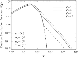
Figure 1.— The electron distribution function $N(\gamma)$ for different choices of $\zeta$. The other model parameters are fixed as shown in the legend. At the cooling break ${\gamma_{\mathrm{b}}}$, the power-law index increases by 1.

Özel et al. (2000) proposed a hybrid thermal-nonthermal model for synchrotron radiation in low-luminosity AGN. When applied to Sgr A*, the hybrid model shows better agreement with observations compared to a pure thermal model. However, recent polarization measurements of Sgr A* show that the rotation measure in the emission region is small, which suggests that the low-energy component of electrons is relativistic and likely thermal (Marrone et al., 2006). We modify the hybrid model so that the nonthermal distribution contributes only at high energies. That is, for some critical value ${\gamma_{\mathrm{c}}}$, we assume

$$N(\gamma)=\left\{\begin{array}[]{lll}{N_{\mathrm{th}}}(\gamma)&,&\gamma<{\gamma_{\mathrm{c}}}\;,\\ {N_{\mathrm{pl}}}(\gamma)&,&\gamma\geq{\gamma_{\mathrm{c}}}\;,\end{array}\right.$$ (11)

where $\gamma$ is proportional to the (ultra-relativistic) electron energy. When most of the electrons are thermalized, our distribution function is a close approximation to the hybrid model of Özel et al. (2000). Otherwise, our modified hybrid model keeps the low-energy electrons in a thermal distribution.

In order to obtain analytical expressions for the normalization, we take the domain of $\gamma$ to be all positive real numbers, and use the ultra-relativistic Maxwell-Boltzmann distribution

$${N_{\mathrm{th}}}(\gamma)={N_{\mathrm{c}}}\frac{\gamma^{2}}{{\gamma_{\mathrm{c}}}^{2}}\exp\left(\frac{{\gamma_{\mathrm{c}}}-\gamma}{\theta_{e}}\right),$$ (12)

where ${N_{\mathrm{c}}}$ is the normalization and $\theta_{e}={k_{\mathrm{B}}}T_{e}/m_{e}c^{2}$ is the dimensionless electron temperature. We use ${k_{\mathrm{B}}}$ to denote the Boltzmann constant, $T_{e}$ to denote the electron temperature, which is assumed to be equal to the plasma temperature $T$, and $m_{e}$ to denote the electron mass. Provided $\theta_{e}\gg 1$, the ultra-relativistic approximation will not introduce an appreciable error. Note that the maximum of the thermal distribution is located at $\gamma=2\theta_{e}$. It is convenient to introduce a parameter

$$\zeta={\gamma_{\mathrm{c}}}/2\theta_{e}\geq 1\;,$$ (13)

and specify it in our model.

We also introduce an additional parameter for the cooling break. The broken power law is given by

$${N_{\mathrm{pl}}}(\gamma)={N_{\mathrm{c}}}\left\{\begin{array}[]{lll}\ \ \ \ {\gamma_{\mathrm{c}}}^{s}/\gamma^{s}&,&\gamma<{\gamma_{\mathrm{b}}}\;,\\ {\gamma_{\mathrm{b}}}{\gamma_{\mathrm{c}}}^{s}/\gamma^{s+1}&,&\gamma\geq{\gamma_{\mathrm{b}}}\;.\end{array}\right.$$ (14)

The power-law index $s$ describes the spectrum of injected electrons and is believed to be greater than unity. Because the synchrotron cooling timescale is proportional to $\gamma^{2}$, the electrons in the high-energy tail cool more rapidly. The parameter ${\gamma_{\mathrm{b}}}$ therefore controls the location of this cooling break.

The symbol ${N_{\mathrm{c}}}$ in the above equations denotes the normalization of the distribution at ${\gamma_{\mathrm{c}}}$. Integrating the distribution, it is easy to show that

$${N_{\mathrm{c}}} = \frac{\rho}{{m_{\mathrm{H}}}}\left\{\frac{2\theta_{e}^{3}}{{\gamma_{\mathrm{c}}}^{2}}\left[\exp\left(\frac{{\gamma_{\mathrm{c}}}}{\theta_{e}}\right)-1\right]-\frac{2\theta_{e}^{2}}{{\gamma_{\mathrm{c}}}}-\theta_{e}+\right.$$ (15)

$$\ \ \ \ \ \ \ \ \ \left.\frac{1}{s-1}\left[{\gamma_{\mathrm{c}}}-{\gamma_{\mathrm{b}}}\left(\frac{{\gamma_{\mathrm{c}}}}{{\gamma_{\mathrm{b}}}}\right)^{s}\right]+\frac{1}{s}{\gamma_{\mathrm{b}}}\left(\frac{{\gamma_{\mathrm{c}}}}{{\gamma_{\mathrm{b}}}}\right)^{s}\right\}^{-1},$$

where $\rho$ is the mass density and ${m_{\mathrm{H}}}$ is the mass of hydrogen.

Figure 1 shows the electron distribution function $N(\gamma)$ for different choices of $\zeta$ with fixed density $n_{e}=\rho/m_{\rm H}$ and temperature. The function approaches a pure thermal distribution as $\zeta\rightarrow\infty$. As we decrease $\zeta$, more and more electrons are placed in the nonthermal tail. Note that the spectral index of the power-law component increases by one at the location of the cooling break ${\gamma_{\mathrm{b}}}$. This modified hybrid thermal-nonthermal model will be used to fit the spectrum of Sgr A* up to the X-ray band in §3.

2.3. Synchrotron Radiation

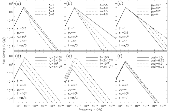
Figure 2.— Dependence on the model parameters of the flux density $F_{\nu}$ observed at Earth. The flux densities are computed from our emission model assuming a simplified disk. The top panels [from (a) to (c)] present the dependence on different parameters in the emission model, while the bottom panels present the dependence on the parameters of the disk itself. The units for $T$ are $\mathrm{K}$; the units for $n_{e}$ are $\mathrm{cm}^{-3}$. The non-monotonic dependence of the spectrum on $\cos i$ is caused by the combined effects of Doppler boosting, projection, and the pitch-angle dependence of the synchrotron radiation.

The emission coefficient in equation (9) is given by

$$j_{\nu} = \frac{\sqrt{3}e^{2}}{2c}\nu_{B}\sin\alpha_{B}\int_{0}^{\infty}N(\gamma)F(x)d\gamma\;,$$ (16)

where $\nu_{B}=eB/2\pi m_{e}c$ is the non-relativistic cyclotron frequency, and $\alpha_{B}$ is the angle between the magnetic field and the line of sight in the comoving frame. Here we use $e$ to denote the electron charge and $B$ to denote the magnitude of the magnetic field. The function $F(x)$ is defined by

$$F(x)=x\int_{x}^{\infty}K_{5/3}(z)dz$$ (17)

(Pacholczyk, 1970), where $x$ is related to $\gamma$ according to $x=x_{0}/\gamma^{2}$, with

$$x_{0}=\frac{2\nu}{3\nu_{B}\sin\alpha_{B}}\;.$$ (18)

We assume that the sub-grid fluctuation of the magnetic field is small. Writing $\mathbf{\hat{B}}=\mathbf{B}/|\mathbf{B}|$, we simply use

$$\cos\alpha_{B}^{\prime}=\mathbf{\hat{B}}\cdot\mathbf{\hat{i}}$$ (19)

to obtain the angle between the magnetic field and the line of sight. The comoving angle cosine is then given by the transformation

$$\cos\alpha_{B}=\frac{\cos\alpha_{B}^{\prime}-\beta}{1-\beta\cos\alpha_{B}^{\prime}}\;.$$ (20)

Using $x_{M}=x_{0}/\theta_{e}^{2}$, the emission coefficient can be written as

$$j_{\nu} = \frac{e^{2}\nu}{\sqrt{3}c}{N_{\mathrm{c}}}\left[\frac{e^{2\zeta}}{4\zeta^{2}\theta_{e}}I_{2\zeta}(x_{M})+\frac{{\gamma_{\mathrm{c}}}^{s}}{2}J_{s,{\gamma_{\mathrm{b}}}}(x_{0},{\gamma_{\mathrm{c}}})\right]\;.$$ (21)

The partial thermal synchrotron function, $I_{2\zeta}(x_{M})$, is given by the integral

$$I_{2\zeta}(x_{M})=\frac{1}{x_{M}}\int_{0}^{2\zeta}z^{2}e^{-z}F\left(\frac{x_{M}}{z^{2}}\right)dz\;,$$ (22)

where $z=\gamma/\theta_{e}$. It does not have any known analytical form. We approximate it by a piecewise power law, i.e., for each fixed $\zeta$, we pre-compute the function numerically as a lookup table and carry out linear interpolations on a log-log scale. Similarly, the function $J_{s,{\gamma_{\mathrm{b}}}}(x_{0},{\gamma_{\mathrm{c}}})$ is given by

$$J_{s,{\gamma_{\mathrm{b}}}}(x_{0},{\gamma_{\mathrm{c}}}) = \frac{1}{x_{0}^{(s+1)/2}}\int_{x_{\mathrm{b}}}^{x_{\mathrm{c}}}x^{(s-3)/2}F(x)dx+$$ (23)

$$\frac{{\gamma_{\mathrm{b}}}}{x_{0}^{(s+2)/2}}\int_{0}^{x_{\mathrm{b}}}x^{(s-2)/2}F(x)dx\;,$$

where ${x_{\mathrm{c}}}=x_{0}/{\gamma_{\mathrm{c}}}^{2}$ and ${x_{\mathrm{b}}}=x_{0}/{\gamma_{\mathrm{b}}}^{2}$. The integrals are related to a class of hypergeometric functions. However, because there is no convergent algorithm to compute this specific class of hypergeometric functions, we will simply perform the integral numerically, for each $s$ and ${\gamma_{\mathrm{b}}}$. We use a piecewise power law to approximate the first integral as a function of ${x_{\mathrm{c}}}$.

Figure 2 demonstrates how the spectrum depends on the different parameters. To highlight the characteristics of the emission model, we assume for illustrative purpose that the disk is uniform and rotates with a constant (dimensionless) azimuthal velocity $\beta=2/3$. We also assume an azimuthal magnetic field, whose energy density is $10\%$ of the internal energy of the gas, and use a disk volume of $4\pi\times 10^{38}\mathrm{cm}^{3}$, which is of the same order as our computational domain (see §4). In the first row of panels, we vary different parameters of the electron distribution. It is interesting to note that in panel (a), the nonthermal tail depends only weakly on $\zeta$ when $\zeta\lesssim 4$. Panel (b) shows how the spectrum depends on the power-law index $s$. Indeed, from equations (21) and (23), it can be seen immediately that the nonthermal tail has a broken power-law spectrum with indexes $(s-1)/2$ and $s/2$. Panel (c) shows the effect of changing ${\gamma_{\mathrm{b}}}$.

The second row shows the dependence of the spectrum on $n_{e}$, the temperature $T$ (note that we assume that the electron temperature is equal to the ion temperature), and the inclination angle of the disk $i$. As the density is increased, the disk becomes optically thin at higher frequencies [see panel (d)]. The optically-thick portion of the spectrum is blackbody-like and is proportional to the projected source size and the temperature. Increasing the temperature will increase the blackbody flux linearly. The emission efficiency in the optically thin portion is proportional to the square of the temperature, which explains the change in shape of the spectrum at $T=3\times 10^{11}\mathrm{K}$ [see panel (e)]. Panel (f) shows the dependence on the inclination angle $i$ of the disk. On one hand, a larger value of $i$ results in a smaller projected source size and a small angle between the magnetic field and the line of sight at the blue-shifted side of the disk, implying less efficient synchrotron radiation. On the other hand, a larger value of $i$ enhances the effect of Doppler boosting. We found that the highest peak frequency is reached when $\cos i=1/2$, which, obviously, depends on the azimuthal velocity we adopt.

3. Observational Constraints

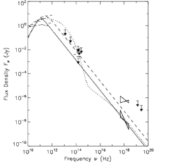
Figure 3.— Model fit to the observed broadband spectrum of Sgr A*. The horizontal bars show only the extrema obtained from different observations, while the arrows at NIR and $\gamma$-ray wavelengths give upper bounds on the flux densities in the quiescent state. We use $T=10^{11}\mathrm{K}$ and $n_{e}=5\times 10^{6}\mathrm{cm}^{3}$ at the outer boundary of the disk. The solid line is the spectrum computed from our emission model with $\zeta=1$, $s=3.5$, ${\gamma_{\mathrm{b}}}=\infty$, and $\cos i=1/2$ from a snapshot at the $t=13$ hr of the quiescent simulation. The dashed line corresponds to the perturbed simulation. To demonstrate that this is not a unique fit, we compute the quiescent spectrum with a temperature that is 10 times higher throughout the disk and $\zeta=10$, $s=2.5$ and ${\gamma_{\mathrm{b}}}=10^{5}$ (the other parameters are the same as the solid line); the result is shown by the dotted line.

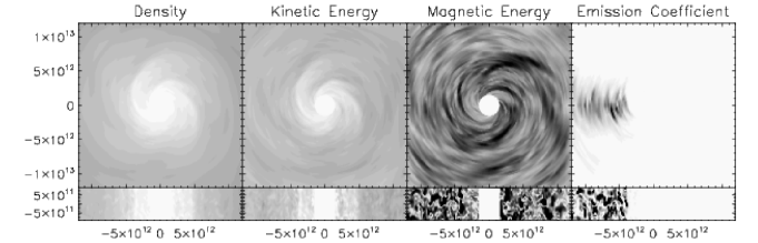
Figure 4.— Gray-scale plots of different quantities in the unperturbed simulation at late time ($t=13$ hr). From left to right the panels show the density $\rho$, kinetic energy density $\rho v^{2}/2$, magnetic energy density $B^{2}/8\pi$, and the emissivity in the infrared ($\nu_{0}=1.8\times 10^{14}\mathrm{Hz}$) band with relativistic corrections ($\cos i=1/2$ in this case, see text for details). The polar plots in the top row are vertically-averaged results, while the rectangular plots along the bottom show the variation with height in the disk. The asymmetry in the effective emission coefficient comes from the Doppler effect.

Figure 3 shows the observed flux of Sgr A* at different frequencies (see Liu et al., 2004, for the instruments and references). The horizontal bars show the maximum and minimum fluxes observed so far at the corresponding frequencies. The arrows at NIR and $\gamma$-ray wavelengths give the upper bounds for the quiescent state emission. Fitting these data, one obtains a (non-unique) set of parameters for the emission model and physical conditions of the accretion disk.

The mm/submm spectrum of Sgr A* has been modeled in different ways by various groups. Narayan et al. (1995) used thermal emission from an advection-dominated accretion flow. Mahadevan (1998) and Özel et al. (2000) incorporated the effects of a hybrid electron distribution in the same model. Melia et al. (2001b) considered thermal synchrotron emission from a compact accretion disk, whereas Markoff et al. (2001) used the emission of a thermal jet. For a magnetic field energy density below equipartition with the energy density of the plasma as suggested by MHD simulations (Hawley, 2000), these studies generally point to an emission region of a few Schwarzschild radii with a plasma temperature of $\sim 10^{11}\mathrm{K}$ and a density of $\sim 10^{6}\mathrm{cm}^{-3}$.

Given the low luminosity of Sgr A*, the accretion flow is radiatively inefficient (Melia, 1992, 1994; Narayan et al., 1995; Yuan et al., 2003, 2004). The temperature of the plasma therefore should be close to its virial value. As mentioned above, we assume for simplicity that the electron and proton temperatures are equal. A realistic treatment of the thermal coupling between the protons and the electrons is not feasible in our time-dependent simulations. For a given outer boundary radius of the accretion disk, the scale height of the disk can be estimated from the virial temperature, and we have only the gas density left as a free parameter.

We take the outer boundary of the accretion disk to be $21.5{r_{\mathrm{S}}}$ in our simulations. We can therefore use the broadband spectrum of Sgr A* to constrain the density at the outer boundary, which determines the density normalization of the whole disk, the inclination angle of the disk, and other parameters describing the nonthermal population of the electrons (specifically, $\zeta$, $s$, and ${\gamma_{\mathrm{b}}}$).

The solid line in Figure 3 is an emission spectrum computed from a late time snapshot (at $t=13$ hr) of our quiescent-state simulation (see § 5 for details) with $T=10^{11}\mathrm{K}$ and $n_{e}=10^{6}\mathrm{cm}^{-3}$ at the outer boundary. The disk inclination angle is $\cos i=1/2$, while the emission model parameters are $\zeta=1$, $s=3.5$, and ${\gamma_{\mathrm{b}}}=\infty$. We note that the spectrum peaks at $\sim 1.2\times 10^{11}$ Hz with a peak flux density of $\sim 3$ Jy. Observations suggest that Sgr A*’s spectrum peaks at $220$ GHz, slightly above the model predicted value, with a flux density of $\sim 3$ Jy (Marrone et al. 2006). In order to better understand this difference, we sampled the parameter space to improve the quality of the fitting. For the chosen snapshot of our quiescent-state simulation, we either over-predict the peak flux density or have a lower peak frequency as shown in the figure. These deviations suggest that the real electron temperature might be lower than the plasma temperature, as also expected on theoretical grounds, while the electron density might be higher than in our calculations; this would shift the simulated emission peak frequency and flux density closer to the observed values. However, quantitative fitting to the spectrum is beyond the scope of this paper, which focuses on the variability of the NIR and X-ray emission. We will adopt the above model parameters in the following sections.

Note that, with ${\gamma_{\mathrm{b}}}=\infty$, we only need two parameters to describe the spectrum of nonthermal electrons. Here we neglect other radiation processes that may dominate in the X-rays (i.e., bremsstrahlung and comptonization). Moreover, at least part of the quiescent-state X-ray emission from Sgr A* is produced near the capture radius of the accretion flow by a thermal plasma (Baganoff et al., 2001, 2003). As a result, the observed X-ray flux needs to be treated as an upper limit for the X-ray emission from our model of the small accretion disk. The above model fitting therefore suggests that for $\zeta=1$, the power-law index can not be less than 3.5. For large values of $\zeta$, one may adopt a small $s$ without violating the X-ray upper limit. These models, however, will predict very weak NIR emission. The parameter ${\gamma_{\mathrm{b}}}$ needs to be included to bring the NIR flux close to the observed values during flares.

The dashed line in Figure 3 corresponds to the perturbed simulation discussed in §6, which predicts an X-ray flare with a soft spectrum and a flux density 8 times higher than the quiescent level. Further analysis of small flares observed by the Chandra and XMM-Newton telescopes are needed to test this prediction. As we pointed out above, the values of model parameters presented earlier do not constitute a unique fit to the spectrum. The dotted line in the figure is another possible fit to the spectrum. The corresponding model parameters are $\zeta=10$, $s=2.5$, ${\gamma_{\mathrm{b}}}=10^{5}$, and $T=10^{12}\mathrm{K}$. The values of the other parameters are the same as those used to produce the solid line.

4. Physical Setup

We take the mass of Sgr A* to be $M=3.4\times 10^{6}M_{\sun}$ (Schödel et al., 2003; Ghez et al., 2003). From the physical conditions in the disk estimated in the previous section, the density and temperature at the outer boundary ($r=21.5\ r_{S}$) are fixed at $\rho_{0}\approx 1.7\times 10^{-18}\mathrm{g\;cm}^{-3}$ and $T_{0}=10^{11}\mathrm{K}$. At this temperature, the plasma is fully ionized, so we take the mean molecular weight to be $\mu=0.5$. We also assume the MHD equations are valid although the electron distribution has a nonthermal component. An absorbing layer is placed between $20{r_{\mathrm{S}}}<r<21.5{r_{\mathrm{S}}}$ to attenuate waves reflecting back into the domain.

In order to focus on the effects of magnetohydrodynamic turbulence produced by shearing, we assume a slab geometry and neglect the vertical component of gravity. Because the disk’s mass is negligible compared to that of the black hole, we also neglect self-gravity. Inflowing (to the black hole) conditions are imposed at the inner boundary at $r=1.5\,{r_{\mathrm{S}}}$, which lies well below the ISCO ($\approx 3{r_{\mathrm{S}}}$) in a Schwarzschild geometry.

At such high temperatures, the electrical conductivity within the plasma is high enough that we can neglect any resistive deviations from ideal MHD (as was done, for example, in the global simulations of Igumenshchev & Narayan, 2002, following the suggestion by Shvartsman 1971). We also neglect molecular viscosity, which is expected to be insignificant compared to the turbulent viscosity arising from Maxwell (and Reynolds) stresses in the magnetized plasma. We take the initial velocity to be Keplerian in a pseudo-Newtonian gravitational potential, $v_{\phi 0}=\sqrt{GMr}/(r-{r_{\mathrm{S}}})$. Shearing leads to the development of the MRI (Balbus & Hawley, 1991).

We start with a uniform density and temperature and an initial magnetic field $\mathbf{B}=B_{0}\mathbf{\hat{z}}$ with $B_{0}=0.3\mathrm{G}$. A random perturbation at the $1\%$ level is added to the temperature, and hence pressure, in order to initiate the MRI. The disk is allowed to evolve towards a quasi-steady state. Note that a linear mode analysis shows that the modes become stable when $k_{z}^{2}>3(\Omega/v_{A,z})^{2}$, so it is important that the computational domain is large enough to enclose unstable modes for which $\lambda_{z}>B_{z}(r-{r_{\mathrm{S}}})\sqrt{\pi r/3GM\rho}$. For our model, the critical value is roughly $0.01r_{S}$ at the inner boundary, and $1r_{S}$ at the outer boundary. Therefore, we choose the vertical domain to be $-r_{S}\leq z<r_{S}$ to ensure that the MRI can develop over the whole disk. We use $257\times 64\times 32$ grid points in our simulations. The vertical resolution can resolve the most unstable wavelength outside the ISCO. The radial and azimuthal grid points are chosen so that these two directions are resolved as accurately as the $z$ direction.

5. Quiescent State

We carry out the calculation described in §4 for 24 simulated hours, which corresponds to about 80 orbits at the ISCO. The material inside the ISCO is accreted very quickly, in under an hour. Magnetohydrodynamic turbulence then kicks in because of the MRI. The inner disk rotates much more rapidly so turbulence is fully developed first in the inner region; the MRI in the outer region grows more slowly. Turbulence is developed through the whole disk by $t=12$ hr (note that the period at the outer boundary is around 6 hours), and the disk reaches a quasi-steady state thereafter.

5.1. Quasi-Steady State Solution

To illustrate the turbulent flow in the disk, we show in Figure 4 gray-scale plots of the density $\rho$, kinetic energy density $\rho v^{2}/2$, magnetic energy density $B^{2}/8\pi$, and the NIR (i.e., $\nu_{0}=1.8\times 10^{14}\mathrm{Hz}$) emissivity. The plots show the disk profile at $t=13$ hr of the simulation, after steady state has been reached. The NIR emissivity is computed with relativistic corrections, using the equation

$$j_{\nu 0}=\left(1-\frac{{r_{\mathrm{S}}}}{r}\right)^{2}\left(\frac{\sqrt{1-\beta^{2}}}{1-\beta\cos\alpha^{\prime}_{v}}\right)^{3}j_{\nu}\;,$$ (24)

where we have assumed a $60^{\circ}$ inclination angle for the disk. The polar plots in the top panels are vertical-averaged quantities. The rectangular plots along the bottom show the vertical structure at the angles $\phi=0$ and $\pi$. Note that the $z$-axis is rescaled to show the vertical structure; the disk itself is much thinner than it appears in these plots.

Because of the high temperature, the density (and the thermal energy, which is not shown in the plots) is rather smooth. The region within $3{r_{\mathrm{S}}}$ is almost empty. Although both the density and kinetic energy decrease inside the ISCO, there is no significant drop in the magnetic field or the temperature there. A weak two-armed spiral pattern, or $m=2$ mode, appears in the density (and thermal energy). This pattern also shows up in the kinetic energy density plot, which is correlated to that of the magnetic field. The turbulent magnetic field shows smaller structure close to the inner disk and larger eddies in the outer region. This agrees with the standard stability criterion of Balbus & Hawley (1991).

The strong asymmetry of the emission coefficient comes from the Doppler shift. Because the plasma moves in a counter-clockwise direction (in the polar plots), the emission from the left side is blue-shifted. The hybrid emission spectrum decreases for frequencies $\nu>10^{11}\mathrm{Hz}$. Hence, blue-shifting raises the emission spectrum and makes the left side of the disk much brighter. In the rectangular plots, the patchy structure of the emission coefficient for $r>4{r_{\mathrm{S}}}$ is well correlated with the magnetic field because $j_{\nu}\propto B^{2}$. For the region inside $4{r_{\mathrm{S}}}$, the low density and low thermal energy, together with the gravitational redshift, reduce the emission coefficient significantly.

5.2. Saturated Turbulent Flow

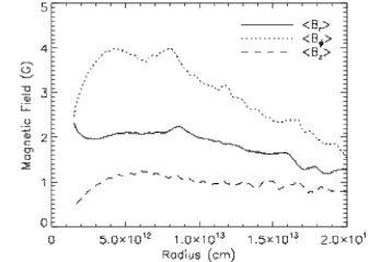
Figure 5.— The root-mean-square of the different components of the magnetic field. Note that, although we start with a seed magnetic field of 0.3 G in the $z$-direction, the magnetic field saturates at a value $\sim 10$ times higher in the (dominant) $B_{\phi}$ component.

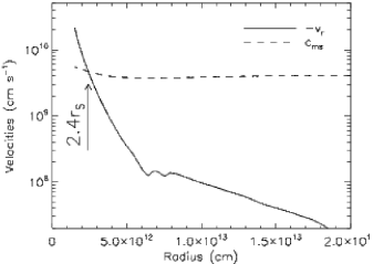
Figure 6.— Average radial velocity (solid) and magnetosonic speed (dashed) profiles through the disk. The intersection of the two lines defines the magnetosonic point $r_{\mathrm{ms}}\simeq 2.4{r_{\mathrm{S}}}$. The fluid inside this point loses causal contact with the outer part of the disk.

In Figure 5, we compute the root-mean-square of different components of the magnetic field

$$\langle B_{i}\rangle_{\mathrm{rms}}=\left(\frac{\int B_{i}^{2}r\;d\phi\;dz}{\int r\;d\phi\;dz}\right)^{1/2}.$$ (25)

Although our initial magnetic field has only a vertical component with a seed value of 0.3 G, the dominant component in the quasi-steady state is $B_{\phi}$. This result is in agreement with earlier global simulations (see Hawley, 2001). The magnitude of the magnetic field (which is dominated by the $\phi$-component) ranges from 2 G near the outer boundary, to the peak value of 4 G near $6{r_{\mathrm{S}}}$, and decreases to about 2.5 G within the ISCO. The magnetic field strength is around 10% of the equipartition value, consistent with the results of Hawley & Krolik (2001, 2002).

Defining an average along the $\phi$- and $z$-directions as

$$\langle f\rangle_{\phi z}=\frac{\int fr\;d\phi\;dz}{\int r\;d\phi\;dz}\;,$$ (26)

the magnetic flux along the radial direction is then given by

$$\Phi_{B_{r}}(r)=\langle B_{r}\rangle_{\phi z}\int rd\phi dz\;.$$ (27)

This should vanish for all radii because of the divergenceless condition of the magnetic field $\nabla\cdot\mathbf{B}=0$ and our periodic $z$-axis boundary condition. We compute $\langle B_{r}\rangle_{\phi z}$ from our simulation and obtain $\langle B_{r}\rangle_{\phi z}\lesssim 10^{-15}\;\mathrm{G}$ at all times. Compared to the root-mean-square values of the different components of the magnetic field, this shows that our algorithm is able to preserve $\nabla\cdot\mathbf{B}=0$ down to machine accuracy. This property is a useful test of our simulation.

The inner edge of the accretion disk should therefore be defined as the location where the infalling material loses causal contact with the rest of the disk. Hence, it may be functionally defined to be the magnetosonic point, at which the radial velocity matches the (fast) magnetosonic speed ${c_{\mathrm{f}}}=\sqrt{{c_{\mathrm{s}}}^{2}+{c_{\mathrm{A}}}^{2}}$, where ${c_{\mathrm{s}}}$ is the sound speed and ${c_{\mathrm{A}}}=B/\sqrt{4\pi\rho}$ is the Alfvén speed. Below this radius, the material loses causal contact with the rest of the disk at larger radii. We plot in Figure 6 the root-mean-square of the radial velocity and magnetosonic speed as functions of radius. The intersection indicates the location of the magnetosonic point, which is around $2.4{r_{\mathrm{S}}}$. The Keplerian period at this radius is 10.76 min, in contrast to the 17.19 min period at the ISCO.

6. Flares

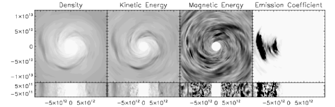
Figure 7.— Same as Figure 4 but for the perturbed simulation.

Earlier hydrodynamic and MHD simulations of the large-scale ($r\gg 20{r_{\mathrm{S}}}$) accretion flow (e.g. Ruffert & Melia, 1994; Coker & Melia, 1997; Igumenshchev & Narayan, 2002, 2003; Cuadra et al., 2005) have indicated that the inflow onto Sgr A* is not smooth. The time scales of these simulations range from 1 to $10^{4}$ years. Given the low-density conditions in the surrounding medium, only parcels of plasma with relatively small specific angular momentum find their way to small radii (Coker & Melia, 1997). The lack of strong accretion apparently inhibits the formation of a large continuous disk extending out to the Bondi-Hoyle capture radius (around $10^{5}{r_{\mathrm{S}}}$). Instead, the compact disk in Sgr A* appears to be accreting clumps of plasma that “rain” inwards from all directions (Falcke & Melia, 1997; Coker, Melia, & Falcke, 1999; Tagger & Melia, 2006).

Each clump circularizes at a radius corresponding to its specific angular momentum. Some clumps presumably reach as far in as the ISCO; most of the others probably merge with the disk at larger radii. To model the impact of such a clump falling onto our quasi-steady inner disk, we simulate its effect on the luminosity of the disk by introducing a density perturbation in the saturated disk.

6.1. Density Perturbation

The perturbation is introduced into the quiescent simulation after quasi-steady state is reached, at $t=12$ hr. The perturbation is Gaussian in density

$$\delta\rho=2\rho_{0}\exp\left(-\frac{r^{2}+r_{0}^{2}+2rr_{0}\cos\phi}{2\sigma}\right)\;,$$ (28)

where $\rho_{0}=10^{6}{m_{\mathrm{H}}}\;\mathrm{cm}^{-3}$, $r_{0}=6{r_{\mathrm{S}}}$ and $\sigma=2{r_{\mathrm{S}}}$. We assume that the perturbation has a temperature of only $10^{10}\mathrm{K}$, much cooler than the disk, to avoid a strong increase in pressure. This allows the clump to move with the plasma in the disk instead of propagating out as sound waves. The internal energy, therefore, is raised by

$$\delta E=\delta\rho\frac{3{k_{\mathrm{B}}}}{2\mu{m_{\mathrm{H}}}}\times 10^{10}\mathrm{K}\;.$$ (29)

For simplicity, we also assume the clump has zero momentum. Hence the velocity is slowed down by

$$\delta\mathbf{v}=\frac{-\delta\rho}{\rho+\delta\rho}\;\mathbf{v}\;.$$ (30)

The simulation is carried out for 10 hours, until the accretion rate becomes comparable to that of the quiescent state again. In Figure 7, we plot the density, kinetic energy density, magnetic energy density, and the effective NIR emission coefficient at $t=13$ hr. The various physical quantities are shown at the same time and with the same gray-scale as in Figure 4 for comparison. The perturbation is sheared out and forms a one-armed spiral pattern in the disk, which also raises the kinetic energy. The correlation between the magnetic energy density and the gas density is less clear in the plot. The perturbation seems to produce a few strong magnetic spots, but it also weakens the $m=2$ mode. There is a prominent feature in the effective emission coefficient; this “hot spot” arises due to both the density and the temperature enhancements.

6.2. Accretion Rate

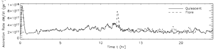
Figure 8.— The variation of the accretion rate $\dot{M}$ at $r=3{r_{\mathrm{S}}}$ with time. The solid line corresponds to the unperturbed simulation. The peak that appears in the first hour is due to our initial condition of a uniform disk. Matter below the ISCO falls into the black hole very quickly after the simulation begins. The dashed line after $t=12\mathrm{hr}$ is the result from the simulation with a density perturbation (see §6). The accretion rate rises for about half an hour, then falls back to the quasi-steady level.

Before looking for quasi-periodic signals in the lightcurve, we first study variations in the accretion rate. In Figure 8 we plot the accretion rate of our simulation at $r=3{r_{\mathrm{S}}}$ as a function of time. The solid line corresponds to the unperturbed simulation, and the dashed line corresponds to the accretion rate after we introduce the density perturbation. The strong peak in the first hour is due to our initial condition of a uniform disk. The material inside the ISCO falls into the black hole immediately after the simulation begins. Although the accretion rate never settles to a constant value, it converges to a value around $2\times 10^{17}\mathrm{g\;s}^{-1}$, consistent with the value inferred from earlier semi-analytic treatments. The weaker peak appearing right after $t=12$ hr is caused by the density perturbation.

Although we do not show it in the plot, the accretion rate $\dot{M}$ at radii $r>6{r_{\mathrm{S}}}$ oscillates between positive and negative values (it actually ranges from $-6\times 10^{17}$ to $1\times 10^{18}\mathrm{g\;s}^{-1}$). These oscillations in $\dot{M}$ have well-defined periods of about 1 hour, though they are not related to the orbital period. They are simply pressure-driven.

6.3. Disk Images

Assuming an inclination angle of $60^{\circ}$ and using the parameters obtained in §3, we integrate the transfer equation along parallel rays and obtain ray-traced images of the accretion disk around Sgr A*. Compared to the emissivity plots in Figures 4 and 7, these images represent the observation more directly because they are numerical solutions of the radiative transfer equation. They also take into account the projection effects of the disk.

In Figures 9 and 10 we present the ray-traced images of our unperturbed and perturbed simulations, respectively. Note, however, that unlike the images provided in Falcke, Melia, & Agol (2000) and Bromley, Melia, & Liu (2001), in which the effects of interstellar scattering and the diffraction-limited finite resolution of the telescope array were taken into account to produce realistic images observed at Earth, these are meant only to show the emission characteristics at the source.

The images show the disk at mm ($10^{11}$ Hz, left), NIR ($10^{14.25}$ Hz, middle), and X-ray ($10^{18}$ Hz, right) wavelengths, from $t=12$ hr (top) to 14 hr (bottom). The K-band is centered on 2.2 microns and has a bandwidth of 0.48 microns. We approximate it by the frequency $1.78\times 10^{14}\mathrm{Hz}$, which is equal to $10^{14.25}\mathrm{Hz}$. The color scales are chosen to enhance the contrast in the emission and are fixed for each frequency. The value of $F_{\nu_{0}}$ given in the plot is the flux density observed at Earth from the whole image, according to equation (2).

From Figure 9, we already see that the accretion disk is highly variable. The flux densities of the unperturbed disk at 12 hr 20 min and 13 hr 40 min are different by a factor of two in both the NIR and X-ray bands. They are only different by about 70% in the mm/sub-mm bump. These variations, due to the bright structure at $10{r_{\mathrm{S}}}$ [panel (b0)], are consistent with the observed frequency dependence of the flux variability. This suggests that the turbulent structure itself can only generate factor-of-two fluctuations. However, although it is not likely to happen, because we have only run the simulation for 24 hours, we cannot rule out the possibility that the turbulence can generate flares that increase the disk brightness by a larger factor, though much more rarely than these smaller variations.

The first row of Figure 10 for the perturbed state is identical to that of Figure 9 because the perturbation is added at $\phi=0$ and $t=12$ hr. The flow shears out the perturbation and forms a one-armed spiral pattern as shown in Figure 7. Not surprisingly, there is a spiral pattern in the corresponding images. At $t=12\;\mathrm{hr}\ 20\mathrm{min}$, we start to see a hot spot appear near the inner edge of the disk. This hot spot is much brighter than the bright structure seen in the unperturbed simulation. The hot spot keeps moving outward due to the leading spiral pattern of the perturbation. One hour after the perturbation is introduced, the disk reaches its brightest moment when its flux is 20% higher than its quiescent value in the radio and 500% brighter in the NIR and X-ray bands.

In addition to the bright one-armed spiral, there are other bright features in the inner part of the perturbed disk. For example, there are two hot spots in the $t=13$ hr image. The inner hot spot moves much faster than the spiral pattern, and appears in the image about every half hour after the perturbation is introduced. These corotating features suggest that QPOs may be found in these simulations.

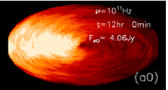
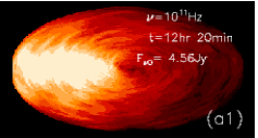
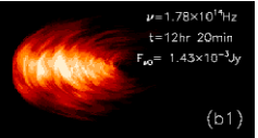
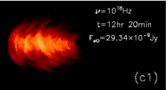
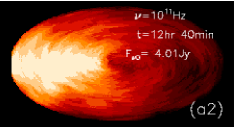
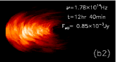
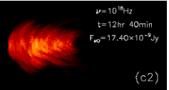
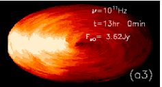
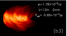
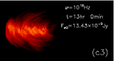
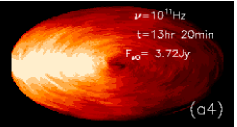
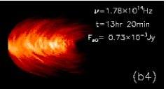
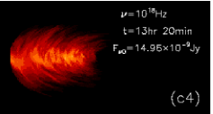
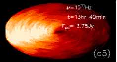
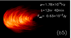
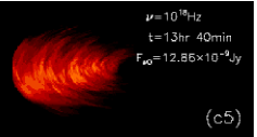
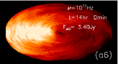
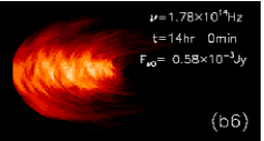
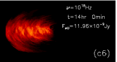
Figure 9.— Ray-traced images of the unperturbed simulation of the accretion disk in Sgr A*. The plots show the images at the thermal peak (left), infrared (middle), and X-ray (right) bands from $t=12$ hr (top row) to 14 hr (bottom). The color scale for each frequency is fixed so that the reader can see the variation of the image with time and compare with Figure 10 for the perturbed simulation. Here, $F_{\nu_{0}}$ is the flux density that would be observed at Earth (from the whole image). Note, however, that these images do not include the distortions produced by interstellar scattering and the finite telescope resolution due to diffraction, and are meant only to convey a sense of the emission geometry at the source.

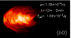
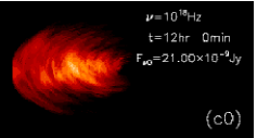
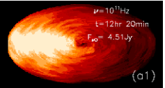
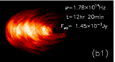
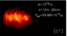
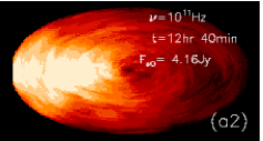
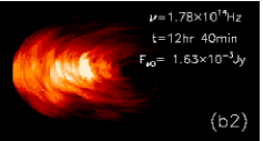
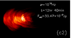
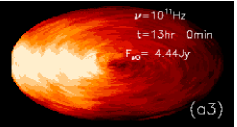
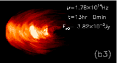
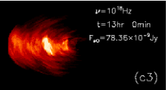
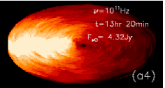
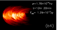
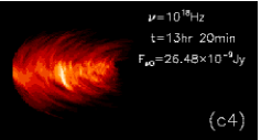
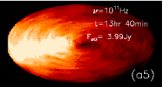
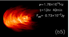
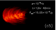
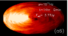
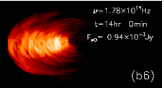
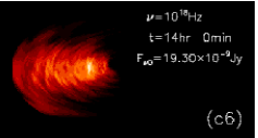
Figure 10.— Same as Figure 9 but for the perturbed simulation.

6.4. Light Curves and QPOs

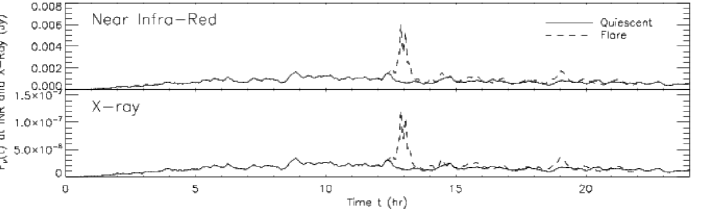
Figure 11.— NIR and X-ray lightcurves. The solid lines are computed from the quiescent state, and the dashed lines are from the flare simulation. Note that the peaks appearing at the 13th hour are much broader than the peak seen in the accretion rate. This indicates that the perturbation actually disturbs the magnetohydrodynamic disk, instead of trivially raising the density. There are some oscillations on top of the peak, which persist all the way to the 20th hour. These oscillations originating from hot spots in the disk produce a QPO in the lightcurve.

In Figure 11, we show the NIR (upper) and X-ray (lower) lightcurves obtained by integrating the flux densities over the disk images. The solid and dashed lines correspond to the quiescent and flare state simulations, respectively.

There are several important differences between the lightcurves shown in Figure 11 and the accretion rate plotted in Figure 8. First, note that the initial peak in the accretion rate in Figure 10 is a transient phenomenon that occurs because the density relaxes from an initial constant value to a steady-state solution. At the same time, the MRI has not yet amplified the magnetic field to produce significant synchrotron radiation. Second, the accretion rate is noisier than the lightcurves because it is a surface integral at some specific radius (at $3{r_{\mathrm{S}}}$ in our case), while the flux density is a volume integral over the whole computational domain. Features with a width $\Delta$ in the accretion disk pass through a specific radius over a time scale $\Delta/v_{r}$; however, they can affect the lightcurve for a much longer time $(r_{\max}-r_{\min})/v_{r}$.

The flare near $t=12$ hr in the perturbed lightcurves lasts much longer than the corresponding peak in the accretion rate. The NIR (and X-ray) flux density reaches its peak at $t=13$ hr, when the accretion rate at $3.0{r_{\mathrm{S}}}$ has dropped back to the quiescent level. These results show that the flux densities are not necessarily correlated with the accretion rate. Indeed, our simulations indicate that the perturbation not only raises the density trivially, but is also able to change the structure of the turbulence. This kind of distortion takes about an hour to develop, and merges with the original turbulent disk within a second hour.

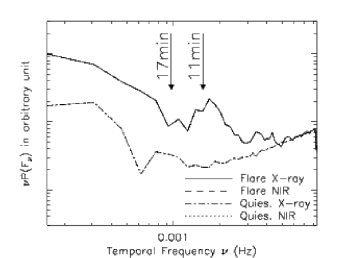
Figure 12.— The PSD (multiplied by the frequency) of the lightcurves. The curves are normalized so that the flat noise spectra at high temporal frequencies match each other. There is no significant period during the quiescent state. In the perturbed simulation, a QPO appears at 11 min, which is the orbital period at $2.4{r_{\mathrm{S}}}$, the magnetosonic point.

Comparing the lightcurves to the disk images, we can identify the second peak of the flare with the hot spots shown in panels (b3) and (c3) in Figure 10. It is directly related to the spiral structure in the disk (see Figure 7). However, the oscillations during the flare, which persist all the way to about $t=20$ hr, come from other features developed by the perturbation—for example, the smaller hot spot located at the inner boundary in panel (b3) of Figure 10.

The evolution of these small fluctuations suggests that there should be a periodic (or quasiperiodic) signal in the lightcurves. In Figure 12, we over-plot the power spectral densities (PSD; multiplied by the frequency) in the NIR band in both the quiescent and flare state simulations. The curves are normalized at higher frequencies for easy comparison of the two. The PSDs of the X-ray lightcurves are almost identical to (and hence overlapping with) the NIR PSDs because both of them are produced by the nonthermal electrons. The two arrows indicate the frequencies associated with the orbital period at the ISCO and the magnetosonic point (at $2.4{r_{\mathrm{S}}}$).

Although there is no significant period in the quiescent state, a QPO-like feature is found in the flare simulation. The quasiperiod is around 11 min, essentially the Keplerian period at the magnetosonic point. This is, to our knowledge, the first QPO seen in magnetohydrodynamic turbulent disks. If such a density perturbation (due to “raining” plasma) is indeed the cause of such flares in nature, the QPOs observed from Sgr A* may be used to set a lower limit on the orbital period at ISCO, and hence provide an estimate of the spin of the Galactic center black hole. This idea can be applied to other low-luminosity AGN as well.

7. Limitations

Although for the first time a QPO is seen in magnetohydrodynamic simulations of accretion disks without invoking special conditions such as large-scale magnetic fields, the QPO period is shorter than that observed from Sgr A*, which is usually longer than 17 minutes (Genzel et al., 2003; Bélanger et al., 2006). This may be partially due to the pseudo-Newtonian potential we have adopted here. In a Schwarzschild geometry, the orbital period at the ISCO for a $3.4\times 10^{6}M_{\odot}$ black hole is 25.7 minutes. If the magnetosonic point is still at $2.4r_{S}$ in such a potential, the corresponding period is 18.4 minutes, which is slightly longer than the period observed in the NIR band but compatible with the X-ray observations (Bélanger et al., 2006). A more complete simulation incorporating general relativistic effects (e.g., Hirose et al., 2004) and relativistic ray tracing calculations (Bromley, Melia, & Liu, 2001) is needed to support more quantitative comparisons with observations.

We also assume a periodic boundary condition along the vertical direction and ignore the vertical component of gravity. Therefore our simulations are only 2.5-dimensional, in the sense that they are able to correctly simulate three-dimensional turbulence but cannot capture many other three-dimensional features. For example, the geometry does not allow an outflow along the vertical direction. Hence, it cannot be used to determine whether there are jets associated with the hot accretion disk, which may contribute to nonthermal radio emission from Sgr A* (Liu & Melia, 2001) and explain the observed correlation between X-ray flares and radio outbursts (Zhao et al., 2004). We also cannot see magnetic-field-dominated funnels as revealed in global relativistic MHD simulations (Hirose et al., 2004). These funnels may be responsible for the acceleration of energetic protons near the black hole (Liu et al., 2006b) and can play an important role in driving Poynting-flux-dominated outflows, which are proposed to power large-scale jets in black hole accretion systems.

The saturation level of our magnetic field agrees with the global simulation of Hawley & Krolik (2001, 2002). Hawley et al. (1995) pointed out that the saturation level of the magnetic field in shearing box simulations depends on the box size. The vertical size of our simulation domain therefore is a free parameter. Stone et al. (1996) also showed that there are more complicated structures in the vertical direction when the effects of gravity are included. A fully three-dimensional simulation is needed to resolve these issues.

To compare observations with MHD simulations, one also has to convert the simulated disk characteristics into a radiation flux spectrum. Observations have already provided good constraints on the emission processes. However, it is not clear how electrons are energized in the turbulent plasma, which is related to the fundamental problem of non-linear turbulence dissipation and electron-ion coupling. In the case of relativistic collisionless plasmas considered here, we lack even the appropriate tools to handle this subject self-consistently. There have been only some phenomenological models developed to address this problem quantitatively (Liu et al., 2004, 2006a; Bittner et al., 2006). In this paper, we have adopted one of the simplest emission models appropriate for the accretion flow in Sgr A* and have used observations to constrain the model parameters. Although the QPO signal is not very sensitive to the model parameters as long as there is a higher energy electron population above the thermal background, one should exercise caution with more quantitative comparisons.

Besides the points mentioned above, there are additional physical processes we can include to improve our simulations and quantitative results. For example, thermal bremsstrahlung, and inverse Compton scattering of the synchrotron photons by the hot electrons may provide a significant contribution to the X-ray emission (Narayan et al., 1995) especially during big flares (Liu et al., 2004).

8. Conclusions

In this paper we have simulated a nonradiative MHD accretion disk around Sgr A* using a pseudo-spectral algorithm. The results are consistent with earlier three-dimensional MHD simulations of the MRI (Hawley & Balbus, 2002), even though we have assumed a different geometry. Our simulations reached a quasi-steady state after the MRI-driven turbulence has fully developed.

We computed the long-wavelength spectrum from our simulation by using a hybrid emission scheme with a thermal background of electrons plus a high-energy nonthermal broken power-law tail. We then used the broadband quiescent-state spectrum to calibrate the model parameters. In the quasi-steady state we found that the source is variable with an amplitude in flux density that increases with photon frequency, in agreement with observations. However, the flux density varied by only a factor two, failing to account for the observed NIR and X-ray flares from Sgr A*.

Motivated by earlier studies of the large-scale accretion processes in Sgr A* (e.g., Coker & Melia, 1997; Cuadra et al., 2005), we introduced a density perturbation to the quasi-steady state disk to see whether they could produce even bigger flux density variations. We found that bigger flares were produced in both the NIR and X-ray bands, as well as a QPO in the lightcurves in association with the magnetosonic point below the ISCO. The fact that the simulated QPO is associated with the magnetosonic point below the ISCO also requires a reexamination of previous estimates of the black hole spin based on flare observations (Genzel et al., 2003; Aschenbach et al., 2004).

References

- Abramowicz et al. (1996) Abramowicz, M.A., Beloborodov, A.M., Chen, X.-M., & Igumenshchev, I.V. 1996, A&A, 313, 334
- Armitage & Reynolds (2003) Armitage, P.J. & Reynolds, C.S. 2003, MNRAS, 341, 1041
- Arras et al. (2006) Arras, P., Blaes, O., & Turner, N.J. 2006,ApJ, 645, L65
- Aschenbach et al. (2004) Aschenbach, B., Grosso, N., Porquet, D., & Predehl, P. 2004, A&A, 417, 71
- Baganoff et al. (2001) Baganoff, F. K., Bautz, M.W., Brandt, W.N., Chartas, G., Feigelson, E.D., Garmire, G.P., Maeda, Y., Morris, M., Ricker, G.R., Townsley, L.K., & Walter, F., 2001, Nature, 413, 45
- Baganoff et al. (2003) Baganoff, F. K., Maeda, Y., Morris, M., Bautz, M.W., Brandt, W.N., Cui, W., Doty, J.P., Feigelson, E.D., Gammire, G.P., Pravdo, S.H., Ricker, G.R., & Townsley, L.K., 2003, ApJ, 591, 891
- Balbus & Hawley (1991) Balbus, S. A. & Hawley, J. F. 1991, ApJ, 376, 214
- Bélanger et al. (2006) Bélanger, G., Terrier, R., De Jager, O., Goldwurm, A., & Melia, F. 2006, astro-ph/0604337, submitted to ApJ
- Bittner et al. (2006) Bittner, J. M., Liu, S., Fryer, C. L., & Petrosian, V. 2006, astro-ph/0608232
- Bromley, Melia, & Liu (2001) Bromley, B.C., Melia, F., & Liu, S. 2001, ApJ, 555, 83
- Chan et al. (2005) Chan, C.K., Psaltis, D., & Özel, F. 2005, ApJ, 628, 353
- Chan et al. (2006a) Chan, C.K., Psaltis, D., & Özel, F. 2006, ApJ, 645, 506
- Chan et al. (2006b) Chan, C.K., Psaltis, D., & Özel, F. 2006, to be submitted
- Coker & Melia (1997) Coker, R. & Melia, F. 1997, ApJ, 488, L1 49
- Coker, Melia, & Falcke (1999) Coker, R. F., Melia, F., & Falcke, H. 1999, ApJ, 523, 642
- Cuadra et al. (2005) Cuadra, J., Nayakshin, S., Springel, V., & Di Matteo, T. 2005, MNRAS, 360, 55
- Falcke & Melia (1997) Falcke, H. & Melia, F. 1997, ApJ, 479, 740
- Falcke, Melia, & Agol (2000) Falcke, H., Melia, F., & Agol, E. 2000, ApJ, 528, L13
- Ghez et al. (2003) Ghez, A. M., Duchêne, G., Matthews, K., Hornstein, S.D., Tanner, A., Larkin, J., Morris, M., Becklin, E.E., Salim, S., Kremenek, T., Thompson, D., Soifer, B.T., Neugebauer, G., & McLean, I. 2003, ApJ, 586, L127
- Ghez et al. (2004) Ghez, A.M., Wright, S.A., Matthews, K., Thompson, D., Le Mignant, D., Tanner, A., Hornstein, S.D., Morris, M., Becklin, E.E., & Soifer, B.T. 2004, ApJ, 601, 159
- Genzel et al. (2003) Genzel, R., Schödel, R., Ott, T., Eckart, A., Alexander, T., Lacombe, F., Rouan, D., & Aschenbach, B. 2003, Nature, 425, 934
- Goldston et al. (2005) Goldston, J. E., Quataert, E., & Igumenshchev, I. V. 2005, ApJ, 621, 785
- Hawley (2000) Hawley, J. F. 2000, ApJ, 528, 462
- Hawley (2001) Hawley, J. F. 2001, ApJ, 554, 534
- Hawley & Balbus (2002) Hawley, J. F. & Balbus, S.A. 2002, ApJ, 573, 738
- Hawley et al. (1995) Hawley, J. F., Gammie, C.F., & Balbus, S.A. 1995, ApJ, 440, 742
- Hawley & Krolik (2001) Hawley, J. F. & Krolik, J.H. 2001, ApJ, 548, 348
- Hawley & Krolik (2002) ——— 2002, ApJ566, 164
- Hirose et al. (2004) Hirose, S., Krolik, J. H., De Villiers, J. P., & Hawley, J. F. 2004, ApJ, 606, 1083
- Igumenshchev & Narayan (2002) Igumenshchev, I.V. & Narayan, R. 2002, ApJ, 566, 137
- Igumenshchev & Narayan (2003) Igumenshchev, I.V., Narayan, R., & Abramowicz, M. 2003, ApJ, 592, 1042
- Kato (2001) Kato, S. 2001, PASJ, 53, 1
- Liu & Melia (2001) Liu, S., & Melia, F. 2001, ApJ, 561, L77
- Liu et al. (2004) Liu, S., Petrosian, V., & Melia, F. 2004, ApJ, 611, L101
- Liu et al. (2006a) Liu, S., Melia, F., & Petrosian, V. 2006a, ApJ, 636, 798
- Liu et al. (2006b) Liu, S., Melia, F., Petrosian, V., & Fatuzzo, M. 2006b, ApJ, 647, 1099
- Markoff et al. (2001) Markoff, S., Falcke, H., Yuan, F., & Biermann, P.L. 2001, A&A, 379, L13
- Marrone et al. (2006) Marrone, D.P., Moran, J.M., Zhao, J.-H., & Rao, R. 2006, astro-ph/0607432
- Melia (1992) Melia, F. 1992, ApJ, 387, L25
- Melia (1994) Melia, F. 1994, ApJ, 426, 577
- Melia & Falcke (2001) Melia, F. & Falcke, H. 2001, ARA&A, 39, 309
- Melia et al. (2001a) Melia, F., Bromley, B. C., Liu, S., & Walker, C. K. 2001, ApJ, 54, L37
- Melia et al. (2000) Melia, F., Liu, S., & Coker, R. 2000, ApJ, 545, L117
- Melia et al. (2001b) ——— 2001, ApJ, 553, 146
- Milsom & Taam (1997) Milsom, J.A. & Taam, R.E. 1997, MNRAS, 286, 358
- Mahadevan (1998) Mahadevan, R. 1998, Nature, 394, 651
- Narayan et al. (1995) Narayan, R., Yi, I., & Mahadevan, R. 1995, Nature, 374, 623
- Narayan et al. (1995) Narayan, R., Mahadevan, R., Grindlay, J.E., Popham, R.G., & Gammie, C. 1998, ApJ, 492, 554
- Ohsuga et al. (2005) Ohsuga, K., Kato, Y., & Mineshige, S. 2005, ApJ, 627, 782
- Özel et al. (2000) Özel, F., Psaltis, D., & Narayan, R. 2000, ApJ, 541, 234
- Pacholczyk (1970) Pacholczyk, A. G. 1970, Radio Astrophysics (W. H. Freeman and Company: San Francisco)
- Psaltis (2003) Psaltis, D. 2003, AIP Conf. Proc, 714, 29.
- Ruffert & Melia (1994) Ruffert, M., Melia, F. 1994, A&A, 288, 29
- Schödel et al. (2002) Schödel, R., Ott, T., Genzel, R., Hofmann, R., Lehnert, M., Eckart, A., Mouawad, N., Alexander, T., Reid, M.J., Lenzen, R., Hartung, M., Lacombe, F., Rouan, D., Gendron, E., Rousset, G., Lagrange, A.-M., Brandner, W., Ageorges, N., Lidman, C., Moorwood, A.F.M., Spyromilio, J. Hubin, N., & Menten, K.M. 2002, Nature, 419, 694
- Schödel et al. (2003) Schödel, R., Ott, T., Genzel, R., Eckart, A., Mouawad, N., & Alexander, T. 2003, ApJ, 596, 1015
- Stone et al. (1996) Stone, J. M., Hawley, J. F., Gammie, C. F., & Balbus, S. A. 1996, ApJ, 463, 656
- Shvartsman (1971) Shvartsman, V. F. 1971, Soviet Astronomy, 15, 37
- Tagger & Melia (2006) Tagger, M. & Melia, F. 2006, ApJ, 636, L33
- van der Klis (2006) van der Klis, M. 2006, Compact Stellar X-Ray Sources, ed. W. H. G. Lewin & M. van der Klis (Cambridge: Cambridge Univ. Press), 39
- Yuan et al. (2003) Yuan, F., Quataert, E., & Narayan, R. 2003, ApJ, 598, 301
- Yuan et al. (2004) ——— 2004, ApJ, 606, 894
- Zhao et al. (2004) Zhao, J.H., Herrnstein, R.M., Bower, G.C., Goss, W.M., & Liu, S.M. 2004, ApJ, 603, L85