Determination of the basic parameters of the dwarf nova
EY Cygni

Abstract

Context. High-dispersion spectroscopy of EY Cyg obtained from data spanning twelve years show, for the first time, the radial velocity curves from both emission and absorption line systems, yielding semi-amplitudes $K_{em}=24\pm 4\,\mathrm{km\,s^{-1}}$ and $K_{abs}=54\pm 2\,\mathrm{km\,s^{-1}}$. The orbital period of this system is found to be 0.4593249(1) d. The masses of the stars, their mass ratio and their separation are found to be $M_{1}\sin^{3}i=0.015\pm 0.002\,M_{\odot}$, $M_{2}\sin^{3}i=0.007\pm 0.002\,M_{\odot}$, $q={K_{1}/K_{2}}={M_{2}/M_{1}}={0.44\pm 0.02}$ and $a\sin i=0.71\pm 0.04\,R_{\odot}$. We also found that the spectral type of the secondary star is around K0, consistent with an early determination by Kraft (1962).

Aims. From the spectral type of the secondary star and simple comparisons with single main sequence stars, we conclude that the radius of the secondary star is about 30 per cent larger than a main sequence star of the same mass.

Methods. We also present VRI CCD photometric observations, some of them simultaneous with the spectroscopic runs. The photometric data shows several light modulations, including a sinusoidal behaviour with twice the frequency of the orbital period, characteristic of the modulation coming from an elongated, irradiated secondary star. Low and high states during quiescence are also detected and discussed.

Results. From several constrains, we obtain tight limits for the inclination angle of the binary system between 13 and 15 degrees, with a best value of 14 degrees obtained from the sinusoidal light curve analysis.

Conclusions. From the above results we derive masses $M_{1}=1.10\pm 0.09\,M_{\odot}$, $M_{2}=0.49\pm 0.09\,M_{\odot}$, and a binary separation $a=2.9\pm 0.1\,R_{\odot}$.

1 Introduction

Dwarf novae are a subclass of cataclysmic variables which have a semidetached late-type secondary star undergoing mass transfer onto a white dwarf primary. Outbursts are frequent in many of these objects, with timescales ranging from a few days to several weeks (see review by Warner war95 (1995)). The spectra of dwarf novae at quiescence usually show strong and broad emission lines of H and He I, while during outburst the same lines are seen in shallow absorption.

EY Cyg is a U Geminorum-type dwarf nova with quiescent V magnitude $\sim$14.8 and outburst V magnitude $\sim$11. Its outbursts have been reported to have a periodicity of about 240 d (Kholopov & Efremov ke76 (1976)) and durations of about 30 d (Piening pie78 (1978)), but a recent analysis of long term AAVSO data may indicate that the system has gone regular outbursts on a 2000 d odd cycle (Tovmassian et al. tea02 (2002)).

EY Cyg has been detected by ROSAT in soft X-rays. Orio & Ögelman (Ori92 (1992)) report a flux of $3\times 10^{-13}$ erg cm^-2 s^-1 in the 0.4-2.2 keV range, and Richman (rich96 (1996)) finds a flux of $1.19\times 10^{-12}$ erg cm^-2 s^-1 in the 0.1-2.4 keV range. Anomalous ultraviolet flux line ratios have been detected by Gänsicke et al. (gea03 (2003)) with HST/STIS; as the authors point out, this may indicate that the system is going through a phase of thermal timescale mass transfer, accreting CNO processed material from the external layers of the secondary star. Recently, Sion et al. (sea04 (2004)) derived an effective temperature of 24,000 K for the primary star, by fitting a white dwarf model to FUSE and STIS spectra.

Strömgren photometry was obtained at minimum light by Echevarría, Costero & Michel (ecm93 (1993)), with values $y=14.79$ and $b-y=0.53$. The colour index indicates a bright secondary of spectral type K, and suggests a very long orbital period system (Echevarría, & Jones ej84 (1984)). 2MASS infrared observations compiled by Hoard et al. (hea02 (2002)) give JHK indices for EY Cyg compatible with those of a KO-K2 star (see their Fig. 4), assuming no interstellar reddening is present. First attempts to obtain a light curve were done by Hacke & Andronov (ha88 (1988)) from photographic observations, and later by Sarna, Pych & Smith (sps95 (1995)) from R and I photometric observations.

Optical spectroscopy dates back to the early observations by Kraft (kra62 (1962)), who pointed out that EY Cyg may have a small velocity variation (close to his detection limit), indicating a system viewed nearly pole-on. The presence of Balmer emission lines and of absorption lines like Fe I $\lambda 4045$ and Ca I $\lambda 4226$, left no doubt as to the binary nature of the system. Kraft classified the secondary as a K0V star. Later, Szkody, Piché & Feinswog (spf90 (1990)) obtained further spectrograms, 12 and 13 days after an outburst, midway between maximum and quiescence. They reported that the spectra revealed strong and narrow emission lines while the absorption lines were still evident. The measured H$\gamma$ and H$\beta$ emission lines yielded no radial velocity curve and no indication as to the spectral type of the secondary star was given. Smith et al. (sscj97 (1997)), from an ISIS spectrum, reported rather weak Balmer and He I emission, a strong red continuum, many absorption features from a red dwarf component, weak TiO bands and rather weak CN lines. No measurements of the emission lines were given and the authors gave a spectral classification of the secondary in the range K5-M0.

A first, tentative orbital period determination of this system was made by Hacke & Andronov (ha88 (1988)), obtaining a period of 0.181228 d. Later Sarna, Pych & Smith (sps95 (1995)), reported a longer orbital period with probable values of 0.2630 or 0.2185 d. The authors argued in favour of the latter value by claiming a dM2-dM3 spectral type of the secondary based on the spectroscopy by Smith et al. (sscj97 (1997)). Preliminary reports of a much larger orbital period (around 0.45 days) were given by Costero, Echevarría & Pineda (cep98 (1998)), Tovmassian et al. (tea02 (2002)) and Echevarría et al. (eea03 (2003)). This larger period is supported by the rate of decline from outburst observed by Kato, Uemura & Ishioka (kui02 (2002)).

In this paper we present and discuss low and high dispersion spectroscopic observations of EY Cyg spanning twelve years, as well as CCD VRI photometric measurements for this object.

2 Observations

Our first observations of EY Cyg were obtained with a Boller & Chivens (B&Ch) spectrograph attached to the 2.1m Telescope of the Observatorio Astronómico Nacional at San Pedro Mártir, during a run from 1993 May 9 to 11, using a 600 lines mm^-1 grating and a 19 $\mu$m Thomson 1024$\times$1024 CCD, to cover a spectral range from $\lambda 5820\,\mathrm{\AA}$ to $\lambda$7500 Å with an spectral resolution of around 3.3 Å. 70 spectra were obtained with 300 s exposure time for each.

Further observations were obtained with the Echelle spectrograph attached to the same telescope. On the nights of 1993 September 25 and 26 the Thomson 1024$\times$1024 CCD was used to cover a spectral range from $\lambda$4080 to $\lambda$6640 Å, with spectral resolution R=18,000. On the subsequent runs (1998 July 13 to 17; 1999 July 22 to 24; 1999 October 3 and 4; 2000 August 22; and 2001 August 28) the Thompson 2048$\times$2048 detector was used to obtain a spectral resolution R=22,000, covering the range $\lambda$3850 – $\lambda$7600 Å. On 2004 July 22 and 2004 October 9 the 1024$\times$1024 SITe3 detector was used at a spectral resolution of R=16,000, covering the range from $\lambda$3800 to $\lambda$6900 Å. All these observations we carried out with the 300 l/mm cross-dispersor, which has a blaze angle at around 5500 Å. Our last run was conducted on 2005 June 26 to July 1 with the Thompson 2048$\times$2048 detector and the 150 l/mm Echellette grating which has a blaze angle around 8000 Å. Exposure times where 900 s for most observations, except a few for which 600 or 1200 s was selected.

VRI photometry was simultaneously conducted during the three nights of the July 1999 spectroscopic run. This was done with the 1.5 m telescope and a Tektronix 1024$\times$1024 CCD. Exposure times for the V, R and I filters were typically 60, 30 and 25 s, respectively. An IRVVRI continuous sequence was conducted. Further I-filter photometry was carried out with the same telescope and a SITe detector on the nights of 2001 August 7, 8 and 30, and V photometry on the nights of 2001 August 28, 29. During the nights of 2004 July 22, 26, 28 and 2005 June 20, 23 and 24, additional I-filter measurements were done with the 0.84 m telescope. More VRI photometry was conducted simultaneously to the spectroscopic observations on 2005 June 25 through July 1, and on July 18, with the same SITe detector on the 1.5 m telescope.

The data was reduced using standard IRAF routines for CCD photometry. Secondary photometric stars, reported in Misselt’s (1996) catalogue, were used; the differential magnitudes reported in this paper are referred to the star identified as number 9 (V=14.630, R=15.069) in that catalogue, which was similar in brightness to EY Cyg during all of our observing runs.

A summary of all the observations is presented in Table 1. Several late-type spectral standard stars, including 61 Cyg A and B, were also observed (mostly during the EY Cygni runs); their published spectral types and radial velocities are listed in Table 2.

Table 1: Observing Log.

Date	Starting HJD	Instr./Tel.	Range(Å)/Band	Resolution/Exp. Time	No. of spectra/images
Spectroscopy
1993 May 9-11	2449117.6	B&Ch/2.1m	5820-7500	2,000	70
1993 Sep 25,26	2449255.7	Echelle/2.1m	4080-6640	18,000	11
1998 Jul 13-19	2451008.0	Echelle/2.1m	3850-7600	22,000	49
1999 Jul 22,23,24	2451381.8	Echelle/2.1m	3850-7600	22,000	39
1999 Oct 3,4	2451454.6	Echelle/2.1m	3850-7600	22,000	17
2000 Aug 22	2451778.8	Echelle/2.1m	3850-7600	22,000	3
2001 Aug 28	2452149.7	Echelle/2.1m	3850-7600	22,000	9
2004 Jul 22	2453208.9	Echelle/2.1m	3800-6900	16,000	3
2004 Oct 9	2453287.7	Echelle/2.1m	3800-6900	16,000	3
2005 June 26-July 1	2453547.9	Echelle/2.1m	3800-6900	22,000	54
Photometry
1999 Jul 22,23,24	2451381.7	Direct/1.5m	VRI	60/30/25	283/288/287
2001 Aug 7,8	2452128.8	Direct/1.5m	I/I	180/180	61/98
2001 Aug 28,29,30	2452149.6	Direct/1.5m	V/V/I	40/40/20	480/447/815
2004 Jul 22,26,28	2453208.7	Direct/0.84m	I/I/I	30/30/30	545/366/197
2005 Jun 20,23,24	2453541.9	Direct/0.84m	I/I/I	30/30/30	155/193/278
2005 Jun 25-Jul 1	2453546.7	Direct/1.5m	VRI	40/40/40	1016/1019/1020
2005 Jul 18	2453569.9	Direct/1.5m	VRI	40/40/40	161/154/160

3 Spectroscopic results

The spectra of EY Cygni show a very narrow H$\alpha$ emission line, as well as a very weak (sometimes absent) H$\beta$ line. Also conspicuous is the combination of the HeI $\lambda 5875$ line in emission and the NaI doublet in absorption around $\lambda 5890$. Many other absorption features are also visible, mainly those due to neutral Calcium, Chromium and Iron.

3.1 Radial Velocities

The spectra obtained with the B&Ch spectrograph show a coherent radial velocity curve, although we were unable to obtain reliable results from them due to two factors: 1) the semi-amplitudes of both components have indeed very low values; 2) the object is in the direction of an extended emission nebula, which makes H$\alpha$ particularly difficult to deconvolve. We have therefore set aside these spectra only for a discussion on the spectral type of the secondary, and use the Echelle observations to obtain the radial velocity curves from the emission and absorption components, as well as the orbital parameters of the binary. Heliocentric corrections have been applied to all calculated radial velocities.

Table 2: Observed Spectral Type Comparison Stars

Name	Radial Velocity	Spectral Type
	($\mathrm{km\,s^{-1}}$)
Low Dispersion
HD175541	18.8	G8 V
HD221354	-22.1	K0 V
HD190404	-2.6	K1 V
HD190007	-28.9	K4 V
HD151288	-31.0	K7.5 Ve
HD147379A	-20.7	M0 Vvar
HD147379B	-24.0	M4
High Dispersion
HR8544, HR8545	-3.3, -6.2	G1 V + G2 V
HR8883	16.1	G4 V
HR8734	-14.0	G8 IV
$\sigma$ Dra	26.7	K0 V
36 Oph B	0.0	K2 V
HR751	23.4	K3 V
61 Cyg A	-64.3	K5 V
61 Cyg B	-64.5	K7 V

3.1.1 Absorption

We have measured the radial velocity of the absorption line system of EY Cyg by cross-correlating its spectra with that of 61 Cyg A independently at two dispersion orders covering the spectral intervals $\lambda\lambda$5200-5400 Åand $\lambda\lambda$5350-5550 Å, hereinafter identified as orders 42 and 41, respectively. In these orders strong Fe I lines – like $\lambda\lambda$5232, 5269, 5270, 5282, 5283, 5324, 5328, 5415, 5434, 5429, 5434, 5447, 5455 and 5477 Å– are present. These and other absorption lines in those orders are used simultaneously with the cross-correlation technique to obtain a radial velocity in each spectrum, with a typical error of about 5 $\mathrm{km\,s^{-1}}$. From our 188 Echelle spectra, 21 were discarded due to their very poor signal to noise ratio. The results derived for the remaining 167 spectra are shown in Tables 3 through 7.

3.1.2 Emission

EY Cygni is in the field of a diffuse, complex emission nebulosity (Tovmassian et al. tea02 (2002); Sion et al. sea04 (2004)). This complicates the process of extracting radial velocities from the emission lines. Furthermore, visual inspection of our original CCD Echelle images shows that the nebular H$\alpha$ emission is not symmetric at both sides of the object’s spectrum. We have therefore applied a careful cleaning procedure to the spectra, in order to subtract the nebular emission before deriving the radial velocities.

Figure 1: The added spectra at the H$\alpha$ emission line region.

To illustrate this problem, we show in Figure 1 the added spectrum around the H$\alpha$ region, using all the available spectra. Since the nebular components were not subtracted, the [NII] emission lines are clearly present, as well as the narrow and stationary nebular H$\alpha$ (FWHM $\sim 1\,$Å) superimposed on a broader (FWHM $\sim 5\,$Å) emission line, blurred here by the radial velocity shifts of the disc along all orbital phases. The broad component is slightly blue-shifted with respect to the nebular emission due to the systemic velocity of the binary (see Table 8 below).

The ”cleaning” of the nebular component was done by fitting, in each individual spectrum, a Gaussian to the narrow component, and then subtracting it from the original spectrum. This procedure gave better results than using sky subtracted spectra. We also visually inspected the spectra obtained by both methods, to check that no residuals of the nebular emission were left on the broader line.

The H$\alpha$ emission line was measured using the standard double Gaussian technique and the diagnostic diagrams described by Shafter, Szkody & Thorstensen (1986), to whom we refer for the details on the interpretation of this diagnostic tool. We have used the convolve routine from the IRAF rvsao package, kindly made available to us by J.R. Thorstensen. The emission line is at times so weak that, in the case of 34 spectra, we were unable to obtain any measurement at all. H$\beta$ was too weak to derive any reasonable results from it. Due to the heterogeneity of our different spectroscopic runs, the ”cleaned” H$\alpha$ spectra were first re-binned to a standard linear dispersion of $0.15\,$ Å  per pixel, a value corresponding to the mean spectral resolution of all runs in that Echelle order. The double-Gaussian program was then run with a FWHM value of $4.5\,$Åfor the individual Gaussians, using a wide range of values for $s$, the separation between Gaussians. The results are shown in Figure 2.

Figure 2: Diagnostic diagram for EY Cyg. The best estimate of the semi-amplitude of the white dwarf is 28 km s^-1, corresponding to s=8.1Å.

Figure 3: Periodogram for the absorption radial velocities of all observing runs.

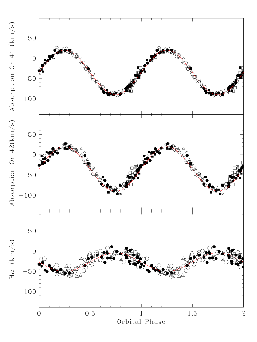
Figure 4: Folded (0.4593249 d) radial velocities for all the observing runs. Top: Absorption lines in Order 41; Middle: Absorption lines in Order 42; and Bottom: H$\alpha$ emission radial velocities. The symbols correspond to: open squares, 1993 September; solid squares, 1998 July; solid circles, 1999 July; open triangles, 1999 October; solid triangles, 2000 August; crosses, 2001 August; asterisks, 2004 July; stars, 2004 October; and open circles, June 2005.

Figure 5: Radial velocity curve for the Junes 2005 run. The symbols correspond to: solid triangles, June 27; dots, June 28; open circles, June 29; open squares, June 30: filled squares, July 1.

As expected from the presence of an asymmetric low-velocity component, the semi-amplitude should asymptotically approach the correct value as $s$ increases. On the other hand, there is a change in slope in the $\sigma(K)/K$ curve when $s$ has reached the line width at the continuum and thereafter the velocity measurements become dominated by noise. The systemic velocity decreases rapidly, up to a value of $s\approx\,8\,$Å, and remains flat afterwards. On the other hand, $K_{em}$ vary very slowly and is the parameter least affected by the different solutions. The best radial velocity results, which are shown in the second column of Tables 3 through 7, are obtained for $s=8.1$Å.

Table 3: Radial velocities for 1993 September 25-26.

HJD	H$\alpha$	Absorption	Absorption
		Order 41	Order 42
(2400000+)	($\mathrm{km\,s^{-1}}$)	($\mathrm{km\,s^{-1}}$)
49255.72620	-6.6	-71.1	-54.1
49255.73800	-5.4	-63.5	-45.4
49255.74981	-0.0	-60.9	-33.2
49255.76439	-22.6	-45.9	-34.4
49255.77619		-34.4	-26.2
49255.78800		-29.6	-26.4
49256.64421		-85.0	-60.2
49256.65601		-81.1	-73.1
49256.66920		-72.8	-43.5
49256.68032	-14.9	-35.0	-30.6
49256.69143	-9.3	-36.0	-38.2
49256.70254		-24.0	-19.6

Table 4: Radial velocities for 1998 July 13-17.

HJD	H$\alpha$	Absorption	Absorption
		Order 41	Order 42
(2400000+)	($\mathrm{km\,s^{-1}}$)	($\mathrm{km\,s^{-1}}$)
51007.95822	-1.4	-78.5
51007.96988	24.1	-90.3	-93.0
51008.86086		-80.0	-55.2
51008.87449		-84.9	-79.1
51008.89246		-88.7
51008.90626		-91.5	-88.2
51008.91954		-86.5
51009.88395	-15.5	-80.1	-79.7
51009.89866	-31.9	-80.0
51009.91316	-31.9	-54.2
51009.93304	-15.6	-23.0	-57.3
51009.94836	-39.3	-35.8	-27.3
51009.96277	-36.5	-27.5	-3.4
51010.77446		-90.1	-74.1
51010.80816		-69.4	-53.2
51010.82181		-63.0	-64.8
51010.89214		-4.2	-19.6
51010.91763			-4.5
51011.68127			-97.7
51011.77820		-48.4	-46.5
51011.80284		-32.8	-10.7
51011.81606			6.1
51011.84696			0.9
51011.86113			5.8
51011.87423		15.3	15.5
51011.88799		14.1
51011.90224			15.3
51011.91574			14.5

Table 5: Radial velocities for 1999 July 22-24.

HJD	H$\alpha$	Absorption	Absorption
		Order 41	Order 42
(2400000+)	($\mathrm{km\,s^{-1}}$)	($\mathrm{km\,s^{-1}}$)
51381.80533	-9.6
51381.82489	-14.6	-74.8	-72.5
51381.86300	-17.0	-86.7	-79.6
51381.87993	-18.0	-90.1	-89.6
51381.93263	-10.2	-74.7	-77.8
51381.97642	-32.7	-42.2	-50.8
51381.99335	-26.3	-43.4	-34.8
51382.66710	-35.2		-2.0
51382.68447	-18.1	-25.7	-21.5
51382.70115	-14.8	-24.5
51382.75382	-3.8	-84.7
51382.77101	-17.2	-85.4	-74.4
51382.85283	-14.3	-72.5	-75.7
51382.86968	-25.2	-70.5	-55.7
51382.88635	-9.6	-59.8	-57.6
51382.90660	-28.4	-47.1	-40.2
51382.92465	-32.2	-31.1	-25.7
51382.94167	-28.2	-17.7	-22.1
51382.96195	-51.0	-6.2	-14.2
51382.97880	-43.1	3.7	5.6
51382.99564	-46.6	19.9	8.5
51383.67261	-27.9		-63.2
51383.68947	-5.9		-76.4
51383.70741	10.8
51383.73015	-0.9
51383.74674	-6.7	-87.8	-76.6
51383.77345	7.1	-74.3	-69.1
51383.79019	1.5	-66.3	-55.3
51383.81866	-15.1	-42.3	-38.5
51383.83534	-18.9	-35.9	-29.8
51383.85230		-18.8	-18.9
51383.86894	-47.1	-11.7	-9.1
51383.88916	-35.7	4.6	5.2
51383.90584	-47.1	6.9	14.2
51383.92257	-50.3	13.0	4.3
51383.93931	-45.8	18.9
51383.96084	-54.9	19.5	27.1
51383.97815	-53.9	20.0	19.8

Table 6: Radial velocities for 1999 October 3-4, 2000 August 22, 2001 August 28, 2004 July 22 and 2004 October 9.

HJD	H$\alpha$	Absorption	Absorption
		Order 41	Order 42
(2400000+)	($\mathrm{km\,s^{-1}}$)	($\mathrm{km\,s^{-1}}$)
51454.63882	-41.9	0.9	8.0
51454.65322	-59.4	12.0	8.7
51454.66637	-52.6	13.6	15.8
51454.68405	-55.0	24.7	23.6
51454.69796	-52.3	20.1	27.6
51454.71122	-57.8	19.5	19.5
51454.72886	-56.2	12.8	11.6
51454.74755	-62.5	9.4	8.6
51454.76506	-60.3	-9.3	-3.7
51455.61267	-38.2	26.8	22.0
51455.62595	-43.5	14.7	17.2
51455.65597	-51.3	9.2	14.4
51455.66984	-42.1	3.6	5.7
51455.68395	-18.7	-0.4	15.0
51455.69785	-29.9	-20.7	6.2
51455.71167	-25.1	-23.1	-12.7
51455.72476	-4.3	-44.2	-22.2
51778.79744	-1.6	-70.3	-70.6
51778.81398	3.9	-66.1	-53.4
51778.84496	-11.4	-40.7	-43.7
52149.66676	-52.4	12.9	13.4
52149.67523	-64.0	14.1	17.8
52149.68299	-50.0	10.8	8.4
52149.78664		-57.4	-51.6
52149.79432		-59.9	-56.0
52149.80199		-69.8	-65.4
52149.88871		-92.5	-93.3
52149.89639	-21.2	-91.7	-96.8
52149.90407	-21.9	-83.8	-96.3
53208.93353	-20.1	-12.0	-13.6
53208.94475		-16.1	-21.7
53208.95631	-9.9	-26.0	-26.8
53287.68969	-16.1	-75.5	-66.7
53287.70084	-18.6	-64.8	-60.7
53287.71199	-25.5	-61.6	-57.8

Table 7: Radial velocities for 2005 June 26 - July 1

HJD	H$\alpha$	Absorption	Absorption
		Order 41	Order 42
(2400000+)	($\mathrm{km\,s^{-1}}$)	($\mathrm{km\,s^{-1}}$)
53547.91137	-37.4	-10.6	-1.1
53547.93209	-22.1	-21.4	-17.9
53547.94793	-12.4	-35.5	-35.4
53547.96377	-14.1	-52.3	-47.7
53548.71897	-49.8	21.4
53548.73562	-47.7	15.6	18.6
53548.75147	-55.2	22.1	19.0
53548.77325	-62.0	16.7	18.4
53548.78910	-50.7	16.9	13.0
53548.80494	-44.8	2.8	11.6
53548.84648	-39.8	-26.5	-16.8
53548.86233	-29.5	-31.5	-29.3
53548.87817	-24.6	-46.2	-36.8
53548.89810	-22.2	-58.2	-52.4
53548.91395	-21.3	-70.8	-62.4
53548.92979	-13.1	-77.6	-75.3
53548.94857	7.6	-86.7	-79.1
53548.96441	-15.3	-92.8	-83.4
53548.98026	-7.3	-88.0	-87.1
53549.69693	-61.4	17.6	21.3
53549.71278	-53.7	4.4	11.4
53549.72862	-42.9	5.3	5.6
53549.76122	-48.4	-10.5	-4.4
53549.77707	-24.1	-28.0	-27.7
53549.79291	-32.5	-46.2	-36.0
53549.81408	-3.0	-55.4	-48.2
53549.82993	-12.2	-65.4	-62.9
53549.84578	-6.8	-70.8	-75.6
53549.88380	-18.2	-84.0	-87.0
53549.89964	-3.7	-84.6	-82.4
53549.91549	-4.2	-83.1	-85.9
53549.93616	-26.8	-77.4	-72.3
53549.95201	-3.6	-77.2	-71.7
53549.96785	-13.6	-66.2	-66.1
53550.71858	-6.7	-39.5	-33.5
53550.73443	-8.3	-57.3	-47.4
53550.75028	-0.0	-68.4	-59.5
53550.85211	-7.5	-84.6	-82.6
53550.86795	0.7	-78.0	-73.3
53550.88380	-27.5	-70.4	-62.7
53550.90879	-28.6	-56.6	-45.1
53550.92463	-39.0	-41.4	-36.6
53550.94049	-40.1	-33.7	-23.8
53552.73156	-9.7	-53.9	-48.5
53552.74756	-3.7	-48.5	-32.5
53552.76341	-11.2	-37.0	-28.3
53552.78316	-19.5	-22.3	-11.3
53552.79900	-18.6	-15.9	-2.0
53552.81485		-6.2	3.8
53552.83491		9.3	13.6
53552.85076	-35.1	26.0
53552.89061	-48.9	15.8	24.3
53552.90648	-37.0	14.9
53552.92232	-40.9	11.2	17.2

3.2 The Orbital Parameters and Radial Velocity Curve

To determine a tentative orbital period we have first made a thorough period search on the absorption radial velocity data, by running a periodgram power spectrum (Deeming 1975). The results are shown in Figure 3 (top), for which the optimum frequency value is 2.177105(80) d^-1, equivalent to a a preliminary period of 0.459333(2) d. On the lower part of the Figure, we show a close-up of the power spectrum region between 2 and 2.5  d^-1 to check for possible aliases between 0.4 and 0.5 days. Based on this period and assuming initial values for the systemic velocity, the semi-amplitudes and the zero point, we then proceeded to obtain the orbital parameters by fitting the measured radial velocities, of both the absorption and the emission data, with sinusoids of the form

$$V(t)=\gamma+K\sin[2\pi(t-\mathrm{HJD_{o}})/P_{orb}]\,,$$

based on a least-squared algorithm. The solutions to the absorption component are very similar for both orders, so we have adopted their average. The results for the absorption and the emission systems are listed in Table 8. The measured radial velocities, together with their sinusoidal fits, are plotted in Figure 4. The data has been folded with an orbital period of 0.4593249 d derived from the solution for the absorption lines, a value which we will adopt hereinafter as the orbital period of the binary. The zero phase correspond to the inferior conjunction of the secondary star. We must point out that the finding of this orbital period value is strongly supported by the fact that during the June 2005 run, we obtained radial velocity data during four consecutive nights and an additional subsequent night (see Table 7), that rule out an alias period, as shown in Figure 5. This is further supported by the photometry of the same four consecutive nights simultaneous to the spectroscopic run, shown in section 4.3 (see Figure 14).

The radial velocity curves in Figure 4 show better results for the secondary star than for the emission line. This is not surprising, considering that the semi-amplitude of the former is almost twice than that derived from H$\alpha$, and the above mentioned complications in obtaining a nebular-free disc emission. All considered, the systemic velocities and orbital periods of both components agree within the errors, although it is possible that we are underestimating the semi-amplitude of the white dwarf as we will discuss below.

Table 8: Spectroscopic Orbital Parameters of EY Cyg.

Orbital	Absorption	H$\alpha$ emission
Parameter
$\gamma$ (km s-1)	-33 $\pm$ 2	-28 $\pm$ 4
$K$ (km s-1)	54 $\pm$ 2	24 $\pm$ 4
$\mathrm{HJD_{o}}$ (2449255 +)	0.3260(9)	0.337(5)
$P_{\mathrm{orb}}$ (days)	0.4593249(1)	0.459323(3)
${\sigma}$	6.8	10.3

Therefore, throughout this paper, we adopt the ephemeris:

$$\mathrm{HJD}=2,449,255.3260(9)\,+\,0.4593249(1)\,E\,,$$

from the inferior conjunction of the secondary star.

3.3 Spectral Type of the Secondary Star

A low dispersion mean spectrum of EY Cyg has been constructed by co-adding the individual B&Ch spectra in the frame of reference of the secondary star, using the orbital parameters in Table 8. The resultant ”absorption enhanced”, or co-added spectrum is shown at the top of Figure 6. At the left, the object is compared with spectra of main sequence stars classified in the range G8 to K4, while on the right, a comparison is made with stars of later spectral types within the range K7.5 to M4. Details of these observed spectral comparison stars, obtained with the same setup as the B&Ch spectra are included in Table 2.

Based on a spectrum obtained by Smith et al. (1997), Sarna, Pych, & Smith (1995) argued that the secondary star corresponds to a spectral type dM2-dM3. However, our co-added EY Cyg spectrum do not correspond to this classification. No traces of TiO bands are present in our spectra, as shown in Figure 6. A comparison of these spectra with our object yields to the conclusion that the spectral type of the secondary star of EY Cyg is that of a late G or early K star. To refine the spectral type we compare the high resolution spectra of the object with a number of spectral type standard stars in the range G8 to K5 (see Table 2).

Figure 6: The mean, low-dispersion spectrum of EY Cyg compared with G8- through M4-type stars.

Since the Echelle spectra are separated in different orders and our observational setup was not intended to add the orders and flux calibrate the overall spectra, we are not able to present similar results as in the low resolution spectra. Instead, we have looked for specific spectral signatures in several orders. The results are shown here for one particularly important spectral region, for which we have co-added a mean spectrum of EY Cyg, in the same manner as in the case of the low resolution spectra. Figure 7 shows the region $\lambda\lambda$4200-4300 Å. A 60 percent flat continuum was subtracted to the spectrum of EY Cyg and rescaled, in order to compensate for the continuum arising from the other light sources in the system. The best lines for spectral classification in stars, which are independent of chemical abundances are the line ratios of the FeI lines $\lambda 4250$, $\lambda 4260$, $\lambda 4271$ Å  to the CrI lines $\lambda 4254$ and $\lambda 4274$ Å, as well as the strength of the CaI $\lambda$4226 Å (Keenan & McNeil 1976; Yamashita et al. 1978). The intensity of the CaI line increase steadily as the spectral type advances (in fact this line has a saturation effect for late K an M stars). On the other hand the CrI lines also increases in strength with respect to the FeI lines with spectral type. These FeI and CrI lines have been marked at the top and bottom of the Figure for clarity purposes. Both the strength of the CaI line and the CrI/FeI ratios of EY Cyg are compatible with a spectral type between G8 and K0. Hereinafter, in accordance with Kraft (kra62 (1962)), we adopt a K0 spectral type for the secondary star.

Figure 7: Co-added Echelle spectrum of EY Cyg in the $\lambda\lambda$4200-4300 Å region, compared with several standard spectral-type stars (see text).

3.4 The $M_{1}-M_{2}$ Diagram

To calculate the masses of the binary one may assume that the semi-amplitudes of the measured radial velocities respresent the true orbital motion of the stars. In cataclysmic variables, however, this may not be an accurate assumption, as the emission lines arising from the disc may suffer several asymmetric distortions (see Wade 1985 for a full discussion on the difficulties in measuring $K_{\mathrm{em}}$). Likewise, absorption line profiles may be subjected to irradiation or hot-spot contaminations in the surface of the secondary, distorting therefore the true value of $K_{\mathrm{abs}}$ (Wade & Horne 1988). These problems were severe in the early determinations of the radial velocities, but modern high resolution spectroscopy has greatly improved the methods in detecting such assymmetries to provide more reliable radial velocity values (Warner 1995). It is important to do the best possible job on the determination of the masses of the binary, because, as mentioned in the introduction, EY Cyg displays a very low C/N abundance ratio, which is expected to be the hallmark of CVs that went through thermal-timescale mass transfer ( Schenker et al. 2002; Gänsicke et al. 2003). If this is correct, one could expect that the white dwarf in EY Cyg grew in mass during that phase - and thus confirming a relatively high white dwarf mass. Taking these into consideration we now attempt to estimate the masses of EY Cyg using the derive radial velocity semi-amplitudes.

Adopting the 0.4593249 d orbital period from the absorption lines solution, and taking

$$K_{1}=K_{em}=24\pm 4\,\mathrm{km\,s^{-1}}$$

and

$$K_{2}=K_{abs}=54\pm 2\,\mathrm{km\,s^{-1}},$$

we obtain:

$$M_{1}\sin^{3}i={PK_{2}(K_{1}+K_{2})^{2}\over 2\pi G}=0.0156\pm 0.002M_{\odot}\,,$$

$$M_{2}\sin^{3}i={PK_{1}(K_{1}+K_{2})^{2}\over 2\pi G}=0.0069\pm 0.002M_{\odot}\,;$$

the projected binary separation

$$a\sin i={P(K_{1}+K_{2})\over 2\pi}=0.71\pm 0.04R_{\odot}\,;$$

and the mass ratio

$$q={K_{1}/K_{2}}={M_{2}/M_{1}}={0.44\pm 0.02}\,.$$

Although EY Cyg is a low inclination binary, for a cataclysmic variable a lower limit and an upper estimate of the inclination angle can be derived by using some reasonable assumptions. To illustrate this, we plot the solutions for the masses of the components as a function of the mass ratio $q$ and the inclination angle $i$. Such an $M_{1}-M_{2}$ diagram is shown in Figure 8. The diagonal solid line correspond to the mass ratio, $q=0.44$, derived in this paper. The adjacent dashed lines are upper and lower limits of $q=0.54$ and $q=0.36$, obtained when the extreme values of the semi amplitudes are used, instead of the error for $q$ quoted above. The dots along these lines correspond to different mass solutions for specific values of the inclination angle. The vertical line is at the Chandrasekhar mass limit and divides the white dwarf degenerate regime from that of neutron stars. This mass limit could be as low as 1.2 $M_{\odot}$ for a high metalicity white dwarf star (Weinberg 1972). The horizontal upper region (shown in grey) is limited by the $M_{2}-P_{orb}$ relation obtained by Warner (1976) using a theoretical ZAMS mass-radius relation (label 1). The other two horizontal limits arise from the mass-radius relation by Echevarría (1983) for 13 spectroscopic and 12 visual binaries with well detached main sequence stars (label 2), and from the $M_{2}-Sp$ and $Sp-P_{orb}$ relations in Kolb & Baraffe (2000) (label 3). The spectral types labelled on the $M_{2}$ axis correspond to masses of ZAMS stars models (left) and to evolved main sequence stars (right), under some extreme assumptions as discussed by Kolb & Baraffe (2000) (see upper curve in their Figure 2). Here, we most stress that the use of these limits and of any mass-radius-spectral type relations, should be taken with great caution. They are used in Figure 8 with the goal to make the $M_{1}-M_{2}$ diagram a useful tool for the analysis of masses in CVs for which only $K_{1}$, $K_{2}$ and the spectral type of the secondary are known. Secondary stars in these systems are almost certainly not main sequence stars (Echevarría 1983; Beuermann et al. 1998). However, if we want to improve on the M-R-Spectral Type relations used in our $M_{1}-M_{2}$ diagram, new and detailed models are needed on evolved main sequence stars and on stars with thermal-timescale mass transfer stages (Shenker et al. 2002; Gänsicke et al. 2003; Sion et al. 2004).

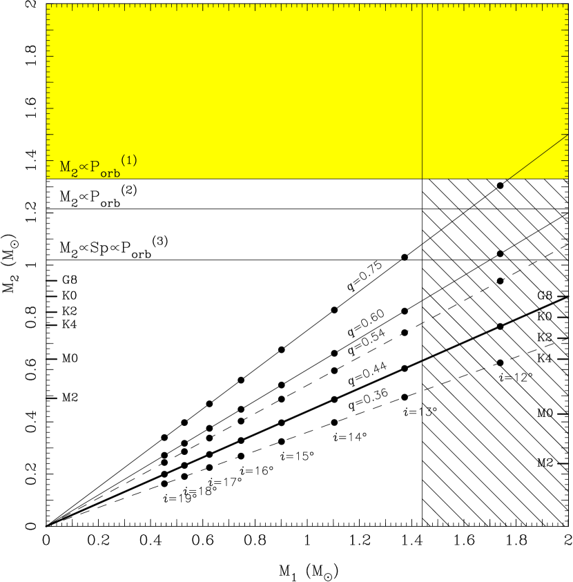
Figure 8: $M_{1}-M_{2}$ diagram. See text for explanation.

From the $M_{1}-M_{2}$ diagram and the above constrains, the inclination angle of the binary cannot be lower than about 13 degrees. Moreover, inclination angles greater than 15 degrees will yield very low masses for the secondary star, incompatible with the observed spectral type. In this respect, the scale of the spectral types, shown in the left of the diagram will move down whether we consider either of two mechanisms. On the one hand, if an evolved secondary is taken into account, then the spectral type for a given mass will be earlier than that of a ZAMS star (see Figure 2 in Kolb & Baraffe kolb00 (2000)), as shown in the right side of the diagram. On the other hand, if we have an X-ray heated secondary – a possibility supported by the detection of soft X-rays in EY Cyg (see the introduction) – then the relative radius of the secondary, as well as its luminosity and temperature, will increase (Hameury et al. 1993) and, consequently, the spectral type will also be earlier than a ZAMS star. For our system we have no independent data that could tell us how much each of these two mechanisms contribute. However the observed spectral type, K0, suggests that both effects contribute significantly. This is evident as the first mechanism alone will yield $i=13^{o}$ only for $q=0.54$. In section 4.2.1 we favour an inclination angle of 14 degrees, based on our observed sinusoidal light curve.

3.5 The radius of the secondary

The secondary appears larger than a ZAMS star for the same mass. The argument is as follows: if we assume that the secondary is a ZAMS star then a K0 spectral type corresponds to $M_{2}=0.87\leavevmode\nobreak\ M_{\odot}$ (Figure 2 in Kolb & Baraffe kolb00 (2000)). This corresponds to a ZAMS star radius of about 0.80 $R_{\odot}$ (Figure 2 in Patterson 1984). However, for a mass of 0.87 $M_{\odot}$ and orbital period of 11.02 h, the radius of the secondary is 1.13 $R_{\odot}$ (equation 4 in Echevarría 1983). The difference is a factor of 1.4.

On the other hand the mass of the secondary, as derived from the radial velocity curves and the best solution for the inclination angle (see section 4.2.1), is $M_{2}=0.52M_{\odot}$. In this case, the corresponding ZAMS radius will be about 0.46 $R_{\odot}$, but now the radius of the secondary from Echevarría’s relation yields 0.96 $R_{\odot}$. The difference is a factor of 2.1.

An increase of the radius of the secondary star by a factor between 1.4 and 2.1 can be explained through the mechanisms discussed above. In the case of an X-ray heated star, the radius can be increased by a factor as large as two (Hameury et al. ham93 (1993)), while an evolved main sequence star scenario also implies a significantly larger stellar radius (Kolb & Baraffe kolb00 (2000)) (see our cautionary statement in section 3.4).

In this respect the case of EY Cyg is similar to the long orbital period system DX And (10.6 h), whose secondary has been found to have a K1V spectral type and a radius a factor of 1.4 larger than a corresponding main sequence star (Drew, Jones & Woods djw93 (1993)).

3.6 The rotational velocity of the secondary

The observed rotational velocity of the secondary star could provide an independent determination on the mass ratio of the binary (e.g. Wade & Horne 1988). The rotational velocity of a semi-detached tidally locked binary is given by:

$$V_{rot}\,\sin i=(K_{em}+K_{abs})\,R_{RL}/a,$$

(Horne, Wade & Szkody 1986), where $R_{RL}/a$ is the Roche-Lobe radius in units of the separation $a$. If we combine this relation with the analytical approximation by Echevarría (1983):

$$R_{RL}/a=0.47469\,[q/(1+q)]^{1/3},$$

based on the tabulations by Kopal (1959) and accurate to 2 per cent for $0.6<q<1.25$, we obtain:

$$V_{rot}\,\sin i=0.47469\,K_{abs}\,q^{1/3}\,(1+q)^{2/3}.$$

Figure 9: Rotational velocity of the secondary star. The symbols correspond to: solid squares, 1998 July; solid circles, 1999 July; open triangles, 1999 October; solid triangles, 2000 August; crosses, 2001 August; asterisks, 2004 July; stars, 2004 October; and open circles, June 2005.

The width of the correlation used to calculate the radial velocities can be used also to derive an observed rotational velocity. To convert the measured $\sigma$ to $V_{rot}\,\sin i$ we have made a calibration by broadening the template star 61 Cyg A, with a suitable rotational kernel for different rotational values. The broadened templates are then cross-correlated with the original template and their $\sigma$ is calculated with a gaussian fit. We have used a simple broadening function for spherical bodies as described by Gray (1976), using a limb darkening coefficient of $\epsilon$ = 0.5 and a bin width of 2.23 km s^-1. A kernel has been produced for a range of $V\sin i$ from 10 to 200 km s^-1 using the IRAF program convolve to broadened the template star.

A plot of the derived values of $V_{rot}\,\sin i$ as a function of phase is shown in Figure 9 for EY Cyg. The width of the correlation was converted to rotational velocities taking into account the spectral resolution, obtained at each observing run, which depend on the detector used and varies from 14 to 18 km s^-1. The Figure shows two clearly distinct values; one with $V\sin i\,\approx$ 50 km s^-1 (filled dots and squares, mainly) and another with $V\sin i\,=$ 34 $\pm$ 4 km s^-1 (open circles only). Using these values and the equation derived above we obtain $q=1.35$ and $q=0.75$ respectively. The first value is incompatible with the radial velocity results and also with the expected value of the secondary mass for a large orbital period system (Echevarría 1983). Furthermore, it is obtained from the observing runs related to the high state (see next section) and its true value may be distorted by heating effects on the secondary, or they may be the result of a large noise dispersion due to the low signal to noise ratio of the absorption lines which are not prominent at these high states. On the other hand, the low rotational value, obtained during the low state (see next section) is more consistent with our radial velocity results, although, a mass ratio of $q=0.75$, imposes more stringent limits in the $M_{1}-M_{2}$ diagram and implies a low primary mass. We have also calculated a mean value of 30 km s^-1 for those observations near orbital phase 0.5 (superior conjuntion) which should be least affected by possible ellipsoidal variations. This value implies $q=0.6$ and $K_{1}=40$ km s^-1, if we keep the calculated $K_{2}$ fixed. This value of $K_{1}$ is still within the maximum and minimum values shown in the H$\alpha$ radial velocity plot in Figure 4. We conclude by arguing that, for this low inclination system, the results of the rotational velocity analysis should be taken only as a cross check on the radial velocity results and not as an independent method of obtaining the mass ratio.

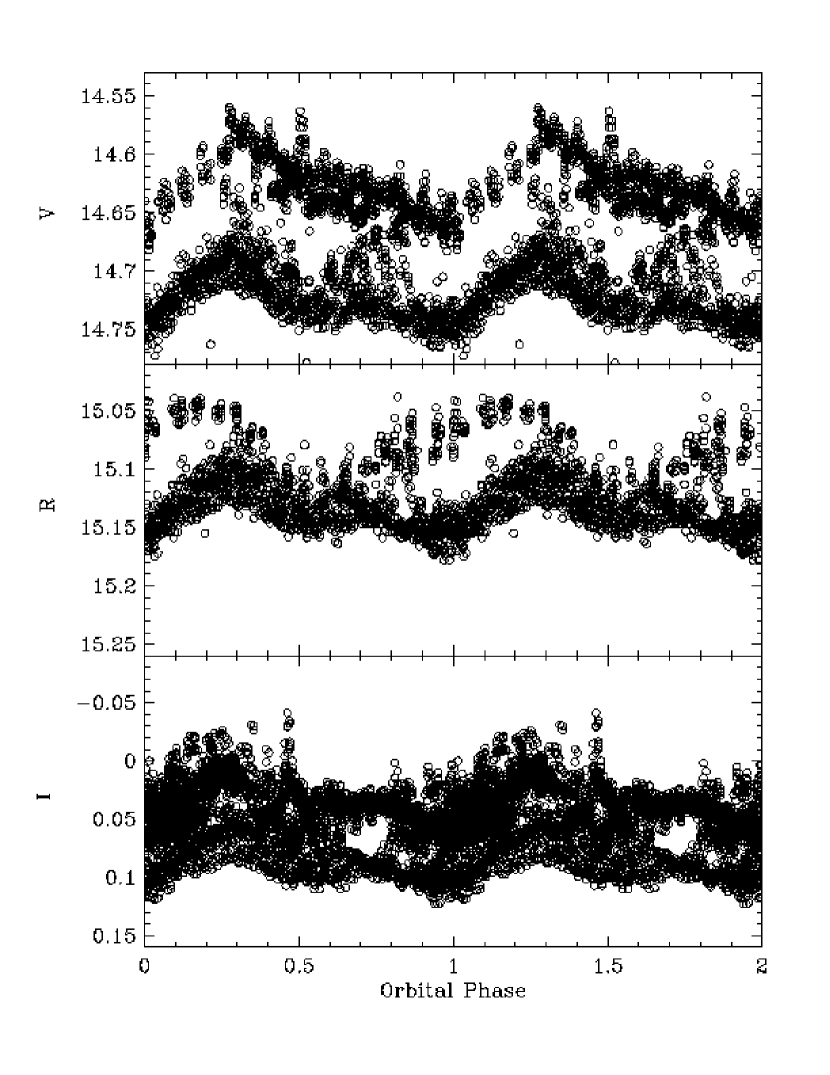
Figure 10: The complete set of our photometric observations folded with the adopted orbital period, all obtained during quiescence. A very complex behaviour is seen, with distinguishable high and low states (see text).

4 Photometric results

Due to the complexity of the light curves observed during several years we have divided the discussion in different sections.

4.1 Overall results

Figure 10 shows our photometric observations of EY Cyg, all obtained during quiescence, folded with the adopted orbital period. These were gathered during several seasons from 1999 to 2005 (see Table 1). The light curves show a modulation of about 0.08 magnitudes, with a general trend to show a maximum around phase 0.25 and a minimum near phase 0.0. We find also that the average brightness of the system varies between seasons. This variation is clearer in V where the change is as large as 0.1 mag. During the fainter states, a lower envelope, reminiscent of the ellipsoidal light variations from an elongated secondary star is clearly seen in all filters (see section 4.3). Other features, less clear in this figure, appear only occasionally and are correlated with the brighter quiescent stages of the object (see section 4.2). We will hereinafter refer to these relatively faint and bright episodes as the low and high states. We must clarify here that this nomenclature refers only to the different light curve behaviour seen during quiescence in this system, and must not be compared with the quiescent and maximum stages in Anti-Dwarf Novae or in Polar systems (Warner 1995). The outburst behaviour in EY Cyg has not been properly studied, as no detailed light curves have been obtained during this stage.

4.2 The high state

In the high state the light curve shows a different behaviour during our different observing runs, like a flat and slow increase immediately followed by a rapid decrease, as well as the opposite behaviour – a rapid increase followed by a slow decrease –, but always with the maximum around phase 0.25 and with no counterpart around phase 0.75 (see Figures 11 to 13). For example, Figure 11 shows that during the 1999 observations, obtained in three contiguous nights and covering most of the orbital phases, the light curve in all VRI filters has a minimum at orbital phase 0.5 and a slow increase up to a maximum at phase 0.25. In contrast to this behaviour, in the V data obtained during two consecutive nights at the end of August 2001 (upper panel in Figure 12 there is again a maximum at phase 0.25, but the brightness now decreases slowly, up to at least phase 0.0 (in this run, there is a gap in the data between this phase and 0.25). The geometrical location of this asymmetric source and its origin are, by no means, obvious. It is a puzzling result which can not be explained by a simple source. If it were a spot on the secondary, it would have to be located on the receding face of the star, which is unlikely, and a hot spot in an accretion disc is expected to be more prominent at phase 0.75. In either case, explanations of this sort are difficult to conceive in a low inclination system like EY Cyg. Perhaps it is more likely to propose a synchronized primary with an accretion column onto its magnetic pole, but this column would have to be about 90 degrees in longitude and at ad hoc latitude. Although synchronization of the primary in polars is possible (e.g. Lamb & Melia 1988; Campbell 1989), studies on the longitude of the magnetic pole show a strong clustering around 20 degrees (Cropper 1988). Nevertheless, polar systems have short orbital periods (¡ 4.6 hr) and, aside from the soft X-ray emission detections in EY Cygni (see introduction) there is no further reason to believe this is a AM Her type object. The possibility of a case for an Intermediate Polar with a slow primary rotator (i.e. close to synchronization with the orbital period) is not completely ruled out by our photometric observations, as they have a limited time coverage. These, and other possible scenarios would have to be tested against new and extensive photometric observations.

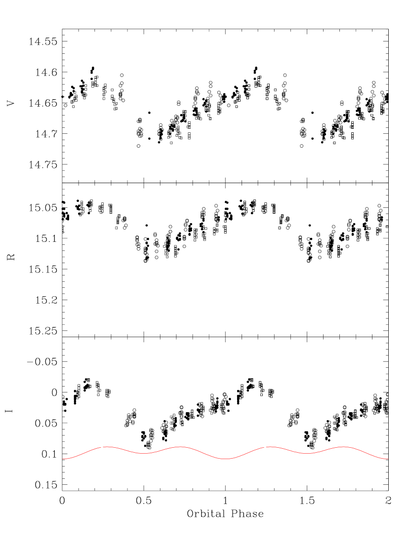
Figure 11: Folded photometric measurements for the July 1999 run. The symbols correspond to: open circles, July 22; solid dots, July 23; and open squares, July 24.

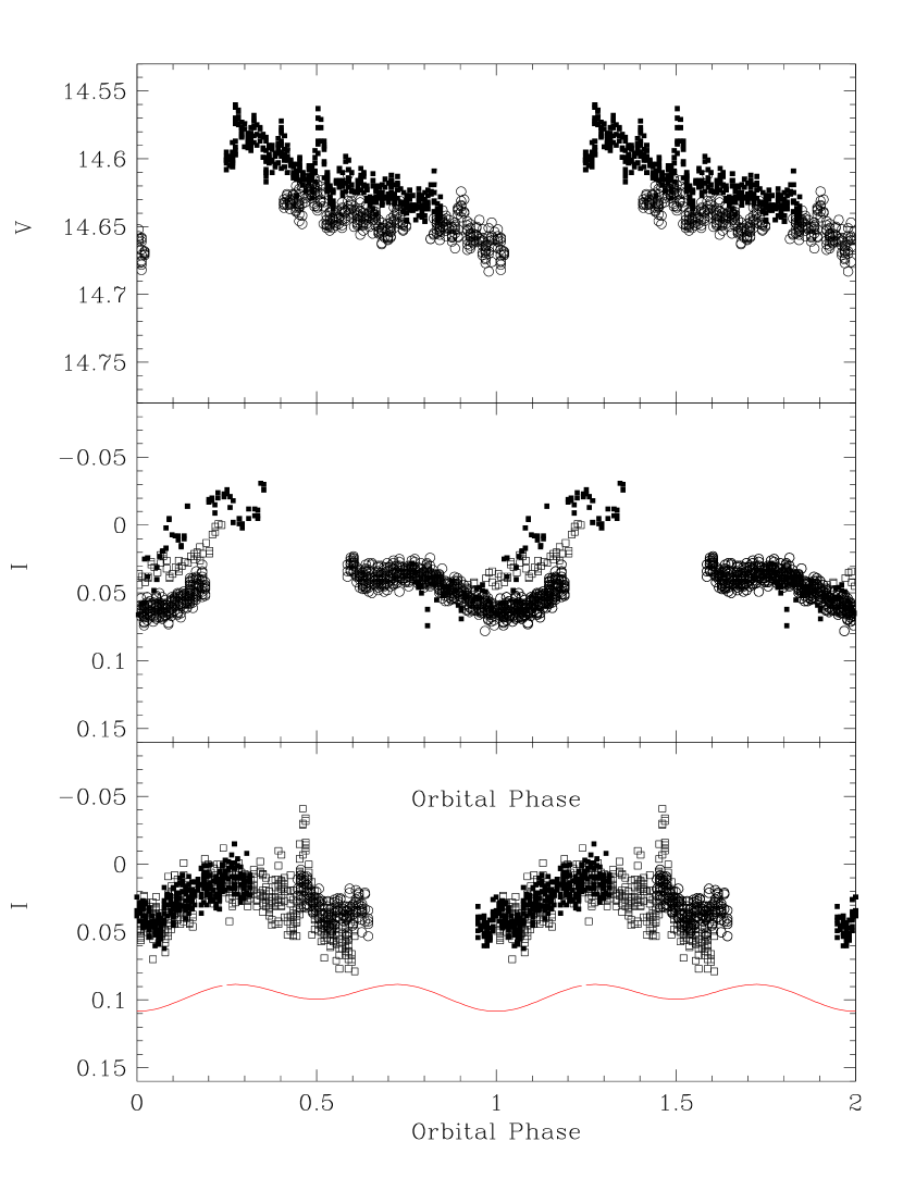
Figure 12: Non simultaneous V and I CCD photometry of the 2001 (upper and midle pannels) and 2004 (lower panel) runs. The symbols correspond to: Filter V (2001, top); solid squares, August 28; open circles, August 29. Filter I (2001, middle); solid squares, August 07; open squares, August 08; crosses, August 30; Filter I (2004, bottom); solid squares, July 22; open squares, June 26; crosses, June 28.

Figure 12 shows non simultaneous observations obtained during 2001 and 2004. We must note that in the V observations on the upper panel, discussed above, the brightness of the object decreases slightly on the second night (August 29) and that in the following night, observed with filter I (crosses, middle panel), we detect a completely new behaviour on the light curve. Instead of the flat and slow increase –or the opposite behaviour–, as that shown in Fig. 11 and in the upper panel in Fig. 12, we now observe a small sinusoidal modulation about 0.1 mag fainter than that seen in 1999 with the same filter. The other two nights, shown in this panel, correspond to earlier observations (August 7 and 8). Although scarce, they follow the high state pattern. In the lower panel of this figure we show further I observations, obtained during three non consecutive nights at the end of July 2004. In spite of the limited phase coverage, the light pattern is again sinusoidal-like, with an intermediate brightness, similar to the I observations of 2001, August 30. These observations appear to be at an intermediate stage between the high and low states.

4.3 The low state and the elongated secondary

Figure 13 shows the 2005 observations obtained while the system was at a low state, most of which were acquired during seven consecutive nights, each of these covering from 6 to 8.2 hours, with a mean of 7.4 hours per night. Being the orbital period 11.0238 days, these data secure a dense and well distributed phase coverage. Even at this low state there is still evidence of the contribution from the light source which shows its maximum around phase 0.25. However, the ellipsoidal modulation of the secondary is now evident. At the lower envelope we observe similar maxima at phases 0.25 and 0.75 – except in filter V –, but different minima at phases 0.0 and 0.5, as expected from a back illuminated elongated secondary. The solid lines in each filter are downshifted solutions to an elongated secondary model.

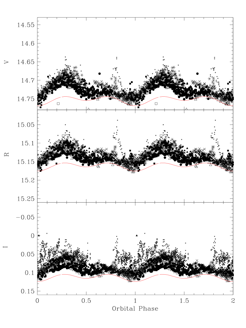
Figure 13: Photometry of EY Cyg during the 2005 run. Each symbol corresponds to a different night. The solid lines are the results of a model for a back illuminated ellipsoidal secondary, shifted downwards in the plots to facilitate their view (see text).

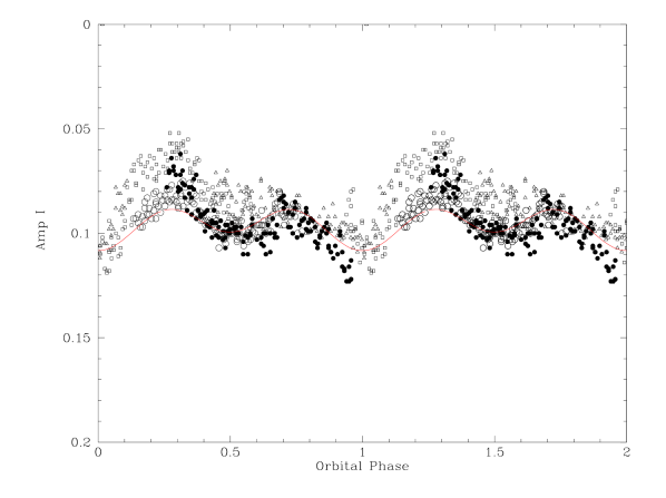
Figure 14: I band CCD photometry of selected nights during the 2005 June run. The symbols correspond to: open squares, June 26; open circles, June 27; dots, June 28; open triangles, June 29.

We show in Fig 14 the I filter data of the two consecutive nights of the above mentioned run, (large open and filled circles), during which the object showed the lowest activity from the asymmetric source. The other five nights in that run show a stronger activity from this source; if used, they will distort the shape of the light curve from the elongated secondary star (discussed in the previous section), and hence produce a spurious effect on the amplitude of this modulation, which is a basically an indicator of the orbital inclination of the binary. To show the level of contamination from this unwanted source, also plotted in the figure are the data from the previous and following nights (small dots and open triangles). In these, we observe that the asymmetric source starts to dominate not only around phase 0.25, but also distorts the minimum at phase 0.5 observed in the two quiet nights. The solid line in this figure is the light curve modelling of the I band data from the two quiet nights, using the program Nightfall (Wichmann W04 (2004)), based on Roche geometry, to simulate the light curve from an elongated secondary.

The fit to the data was obtained using the following main assumptions and program options: a) simple binary system model with a circular orbit and synchronous rotation; b) adopted orbital period and mass ratio calculated in section 3.2; c) Roche-Lobe-filling secondary star with $\mathrm{T}_{\mathrm{e}ff}=4750K$ (corresponding to a spectral class K0)and primary star with $\mathrm{T}_{\mathrm{e}ff}=22,000K$ (Sion et al. sea04 (2004)); d) for the calculation of the heating effect on the secondary star, the bolometric albedo was fixed to 1.0 for the primary and 0.5 for the secondary.

The I light curve fit, shown in Fig 13, is the same as the one shown in Fig 14, but has been slightly shifted downwards for clarity purposes, whereas the V and R light solid curves are the calculated results from the program, and are not fits to the corresponding observations. These calculations are in qualitatively good agreement with the observations.

The best fit solution for the RV curve and the I band data is for an inclination angle of 14 degrees. With very scarce data at a minimum state and probably still contaminated by other light sources, we cannot claim precision to fit the light curve of an elongated secondary. Therefore the result for the inclination angle, in particular, is taken simply as a best choice which is consistent with the constraints derived in the $M_{1}-M_{2}$ diagram (see section 3.4).

5 Masses of the binary

We make some final remarks on the masses of the binary, using the tight limits on the inclination angle discussed in section 3.4. If we use the sinusoidal results from the photometric fit, from which an inclination of 14 degrees yields the best solution, the following masses are derived: $M_{1}=1.10\pm 0.09\,M_{\odot}$, $M_{2}=0.49\pm 0.09\,M_{\odot}$. This favours a massive primary in support of Costero et al. (cep98 (1998)) and Sion et al. (sea04 (2004)). The binary separation in this case would be $a=2.9\pm 0.1\,R_{\odot}$. If we take the upper limit for the mass of the primary, set by the Chandrashekar limit, then the mass of the secondary is around 0.64 $M_{\odot}$, with a corresponding ZAMS spectral type of M0 or an evolved K4 in the extreme case discussed by Kolb & Baraffe (2000). The latter will be more in agreement with our observed spectral type. On the opposite extreme, if we set the inclination angle to 15 degrees, we obtain $M_{1}=0.9\,M_{\odot}$ and $M_{2}=0.4\,M_{\odot}$. The spectral type of the secondary, in this case, would have to be later than M0 in disagreement with the observations.

6 The distance to the system

A rough estimate on the distance to EY Cyg can be made on the assumption the the radius of the secondary appears to be larger than a normal K0 main sequence star. If we take our spectral standard $\sigma$ Dra as the basis for absolute magnitude $M_{V}=5.87$ (e.g. see Luck & Heiter 2005) and assume that the secondary star contributes 50 per cent of the total flux at visual wavelengths –a reasonable extrapolation from the results in section 3.3- then taking $m_{V}=14.75$ (see Figure 13), we obtain $m_{V}(sec)=15.5$. The absolute magnitude for the star with radii 1.4 and 2.1 larger than the normal K0V star are $M_{V}=5.14$ and $M_{V}=4.36$ respectively. These values lead to distances of 1,180 and 1,770 parsecs respectively. At these distances, the interstellar extinction should play a distintive role. Unfortunately, the available IUE spectra (e.g. la Dous 1990) are too noisy to allow a determination via the $\lambda\leavevmode\nobreak\ 2200$ Å dip. On the other hand, a determination using an E(B-V) excess is unwarranted. In fact the observed (B-V)=0.73 (Misselt (1996) is bluer than that of a $\sigma$ Dra, (B-V)=0.79 or that of the general calibration for a KOV star, (B-V)=0.82 given by Johnson (1966). This does not mean that there is no interstellar extinction, but simply that the latter is cancelled by the blue continuum excess that masks the true magnitude value of the secondary star. We have made above a first order estimate of the contribution of this source at visual wavelengths. We can also make a first order estimate of the interstellar extinction. If we assume a value A_V = 1 mag/kiloparsec our distances calculated above are reduced to about 800 pc and 1,200 pc respectively. These values are still larger than upper limit of 700 pc set by Sion et at. (2004), based on the X-Ray luminosity and the background Cygnus supperbubble. We conclude that there are too many uncertainties in the case of EY Cyg to give a reliable distance estimate. This distance determination is important in the composite accretion disc and white dwarf analysis from the FUSE and HST observations by Sion et al. (2004). Unfortunately we are unable to favour any of their models in particular, which are distance dependent, as our method to determine the distance to the system does not improve previous determinations.

7 Summary

The most important results of our study can be summarised as follows:

1. We have been able to detect, for the first time, the radial velocity curve of EY Cyg of both the emission and absorption components, their analysis yielding semi-amplitudes $K_{em}=24\pm 4\,\mathrm{km\,s^{-1}}$ and $K_{abs}=54\pm 2\,\mathrm{km\,s^{-1}}$.

2. From the analysis of the spectral data obtained during 12 years, an orbital period of 0.4593249 d is found.

3. We also find that the spectral type of the secondary star is near K0, consistent with an early determination by Kraft (1962). The secondary contributes around 40 per cent to the total light near $\lambda 4300\,$Å, and has a radius larger than a main sequence star of the same mass by a factor between 1.4 and 2.1.

4. From the Chandrasekhar limit and the observed spectral type of the secondary, tight limits can be imposed to the inclination angle of the binary system, with values between 13 to 15 degrees.

5. The light curve of the system in quiescence shows a complex behaviour, in which we have identified high and low states. At the latter, we detect a phase modulation with twice the frequency of the orbital phase, which can be explained by the effect of an elongated Roche-lobe filling secondary star. During the high state the light curve is characterized by the presence of an asymmetric source around phase 0.25 whose behaviour is different from one observing run to the other. We have discussed possible interpretations for this phenomenon, but we conclude that new and extensive photometric observations are needed, before advancing a convincing explanation.

6. From the ellipsoidal fit to the lower envelope of the light curve we have derived an inclination angle of 14 degrees, which yields masses $M_{1}=1.10\pm 0.09\,M_{\odot}$, $M_{2}=0.49\pm 0.09\,M_{\odot}$, and a binary separation $a=2.9\pm 0.1\,R_{\odot}$.