The cosmic X–ray background and the population of the most heavily obscured AGNs
Abstract
We report on an accurate measurement of the CXB in the 15–50 keV range performed with the Phoswich Detection System (PDS) instrument aboard the BeppoSAX satellite. We establish that the most likely CXB intensity level at its emission peak (26–28 keV) is 40 keV cm-2 s-1 sr-1, a value consistent with that derived from the best available CXB measurement obtained over 25 years ago with the first High Energy Astronomical Observatory satellite mission (HEAO–1; Gruber et al. 1999), whose intensity, lying well below the extrapolation of some lower energy measurements performed with focusing telescopes, was questioned in the recent years. We find that 90% of the acceptable solutions of our best fit model to the PDS data give a 20–50 keV CXB flux lower than erg cm-2 s-1 sr-1, which is 12% higher than that quoted by Gruber et al. (1999) when we use our best calibration scale. This scale gives a 20–50 keV flux of the Crab Nebula of erg cm-2 s-1, which is in excellent agreement with the most recent Crab Nebula measurements and 6% smaller than that assumed by Gruber et al. (1999). In combination with the CXB synthesis models we infer that about 25% of the intensity at keV arises from extremely obscured, Compton thick AGNs (absorbing column density cm-2), while a much larger population would be implied by the highest intensity estimates. We also infer a mass density of supermassive BHs of M⊙ Mpc-3. The summed contribution of resolved sources (Moretti et al. 2003) in the 2–10 keV band exceeds our best fit CXB intensity extrapolated to lower energies, but it is within our upper limit, so that any significant contribution to the CXB from sources other than AGNs, such as star forming galaxies and diffuse Warm-Hot Intergalactic Medium (WHIM), is expected to be mainly confined below a few keV.
1 Introduction
The cosmic X-ray background (CXB) is contributed mainly by active galactic nuclei (AGN) powered by accreting supermassive black holes at the centers of large galaxies (Setti & Woltjer 1989; Comastri et al. 1995; Gilli 2004). Optically bright quasars and Seyfert galaxies dominate at low energies (up to a few keV), while obscured AGNs, which outnumber unobscured ones by a factor 3–4 (Ueda et al. 2003; La Franca et al. 2005), are responsible for the bulk of the CXB at high energies (10 keV). However the CXB intensity level is still a matter of debate. After the first pioneer CXB measurements (Horstman et al. 1975), the major effort to get a reliable estimate of the spectrum in a broad energy band (2–400 keV) was performed in the late 1970’s with the A2 and A4 instruments aboard the first High Energy Astronomical Observatory (HEAO–1). The A2 results (3–45 keV) were first presented by Marshall et al. (1980, hereafter M80), while the final results obtained with the A4 Low Energy Detector (LED, 13–180 keV) were reported by Gruber et al. (1999, hereafter G99), who also presented the conclusive results from both experiments. According to these authors the CXB energy spectrum in the 3–60 keV interval is well represented by a power-law (PL) with a high energy exponential cutoff (cutoffpl), while the corresponding spectrum shows a characteristic bell shape with a maximum intensity of 42.6 keV (cm2 s sr)-1 at 29.3 keV.
After HEAO–1 there have been many other CXB measurements at low energies (15 keV) with both imaging and non imaging telescopes aboard satellite missions, but at high energies (15 keV) no accurate measurement has been published yet. A major effort has been recently performed with INTEGRAL (Churazov et al. 2006). In this case the CXB measurement was obtained by leaving the Earth disk (angular size of as seen by the satellite) to cross the much larger field of view (FOV) of the satellite mask telescopes and fitting the depression in the count rate with a multi-component model, in which one of the components was the CXB and the others were several, e.g., the Earth X-ray albedo, the instrumental background, the celestial sources in the FOV. The many assumptions about the contribution, at the epoch of the measurement, of all the components to the depression level and its dependence on energy and time, make this measurement somewhat difficult for an unbiased estimate of the CXB. Indeed Churazov et al. (2006) wish further INTEGRAL observations at other epochs ”to verify the agreement of observations and predictions”.
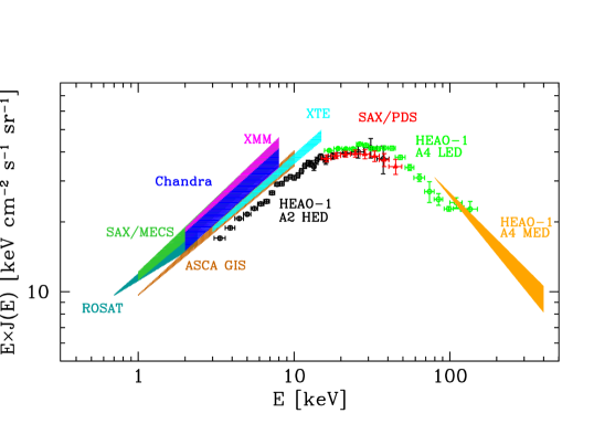
In Table The cosmic X–ray background and the population of the most heavily obscured AGNs we compare the major CXB results. At low energies (1–15 keV), it is apparent a low spread of the pl photon index and a high spread (up to 40%) of the CXB intensity, exemplified by the ratio between the measured 2–10 keV intensities and that measured with HEAO–1, with the lowest CXB estimates obtained with HEAO–1 A2 (M80) and the highest with the focusing telescopes aboard BeppoSAX (Vecchi et al. 1999), XMM-Newton (Lumb et al. 2002; De Luca & Molendi 2004) and Chandra (Hickox & Markevitch 2006). The ratio () obtained with the collimated Proportional Counter Array aboard Rossi–XTE (Revnivtsev et al. 2003) and that () obtained from the re-analysis of the HEAO–1 A2 measurement (Revnivtsev et al. 2005) can be lowered to 1.04 and 1.07, respectively, by a more reliable calibration of the flux scale. Indeed the adopted 2–10 keV Crab flux (Zombeck 1990) is 11% higher than the mean value of all other Crab flux estimates. In the 20–50 keV energy band, which is common to the high energy X–ray experiments, the few available measurements show a low spread of the ratio but systematic errors in the CXB intensity estimates cannot be excluded.
Driven by these discordant results several authors (Ueda et al. 2003; De Luca & Molendi 2004; Comastri 2004; Worsley et al. 2005; Ballantyne et al. 2006; Hopkins et al. 2006; Worsley et al. 2006), in their evaluation of the fraction of the CXB that can be resolved into individual sources or in their CXB source synthesis models, assume the 3–60 keV CXB spectrum obtained with HEAO–1 (G99) to be corrected in its shape, but underestimated in its intensity due to systematic errors in the absolute area calibration and/or instrumental background subtraction. As a result, the HEAO–1 CXB intensity is increased upward by a factor up to 1.3–1.4 over the entire energy band.
In order to establish whether such CXB intensity renormalization is justified, and thus to constrain the size of a population of highly obscured AGNs and to infer the presence of other source populations and/or of a truly diffuse component (WHIM, see Kuntz et al. 2001), we have performed an accurate measurement of the total (resolved plus unresolved) high energy (15 keV) CXB intensity by exploiting the pointed observations performed with the Phoswich Detection System (PDS) aboard the BeppoSAX satellite (Boella et al. 1997a).
2 Instrument and calibrations
A detailed description of the PDS instrument and its in–flight performance can be found elsewhere (Frontera et al. 1997a, b). Although the PDS was not designed to perform a measurement of the CXB (Field of View, FOV, of only 13 FWHM), a posteriori it was realized that such measurement would be possible given the very good performance of the instrument: high temporal stability, very low background level counts (cm2 s keV)-1, high flux sensitivity and good energy calibration. The 15–300 keV limiting sensitivity corresponds to about 1% of the background level with a marginal influence (0.3%) of systematic errors in the background subtraction, also thanks to the continuous monitoring of the background with two rocking collimators which alternated with a default dwell time of 96 s between the neutral position (ON–source) and two default symmetrical positions offset by (OFF–source).
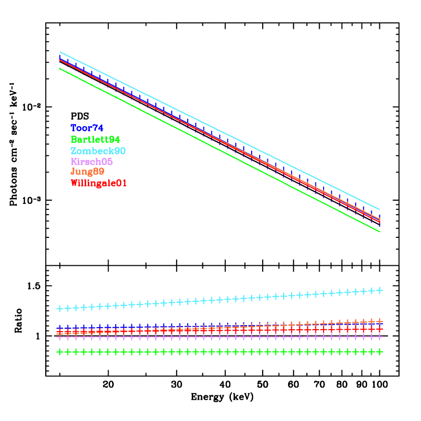
The ON–axis PDS response function was determined by means of pre–launch calibrations combined with Monte Carlo calculations, and it was tested during the BeppoSAX life time (6 yrs) with 7 repeated observations of the Crab Nebula (twice in 1997 and 1999, and once in the years 1998, 2000, and 2001) that were performed simultaneously with the other Narrow Field Instruments (NFIs) on board. By assuming a power–law (pl) model of the form photons cm-2 s-1 keV-1 it was found that the photon index obtained with the PDS remained unchanged in all of these observations within the statistical uncertainties, with a mean value of and a reduced for 66 degrees of freedom (dof) in the 15–200 keV band. A better fit ( for 64 dof) in this energy band was obtained with a broken power-law (bknpl) with a mean low energy index , a break energy keV and a high energy index . A bknpl spectrum was also the best fit to other broad band high energy measurements (see, e.g., Bartlett 1994). The still high obtained with the bknpl model can be lowered and made compatible with the statistics if a systematic error of only 1% in the used PDS response function is assumed.
A cross–calibration of the PDS and MECS telescopes (see, e.g., Boella et al. 1997b) performed with the Crab has provided a time averaged normalization ratio at 1 keV between PDS and MECS of and under the assumption of a pl or a bknpl model, respectively. When corrected upward for this normalization ratio, the mean value of the pl normalization parameter is = , while for a bknpl. A comparison of this Crab spectrum with that obtained with other instruments (see Fig. 1) shows that this renormalized PDS spectrum is consistent within 8% with the extrapolation of the 0.3–10 keV spectrum obtained with the XMM-Newton EPIC–MOS camera (Willingale et al. 2001), with the Crab spectrum obtained with HEAO–1 A4 (Jung 1989) and with the classical Toor & Seward (1974) results. In addition it is in excellent agreement with the mean value of Crab spectrum quoted by Kirsch et al. (2005). As can also be seen from Fig. 1, with respect to the Crab 15–50 keV spectrum obtained with the PDS, that quoted by Zombeck (1990) is higher by %, while that reported by Bartlett (1994) is lower by %. In the following we assume the renormalized Crab spectrum as our calibration scale for the CXB estimate.
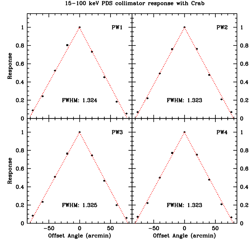
The OFF–axis response function of the PDS was tested with the Crab Nebula during the BeppoSAX Science Verification Phase. The Crab was observed in September 1996 at different offset angles with respect to the instrument axis and with a roll angle such as to get the narrowest angular response of the hexagonal collimators. Results of those measurements were reported (Frontera et al. 1997a) and now confirmed (see Fig. 2). Up to 100 keV the angular response of each PDS unit to the Crab is well fit by a triangular function as expected. The derived FWHM is , which is fully consistent with that derived in the pre-flight tests (Frontera et al. 1997b). We also found that the response function is independent of the offset angle apart from the exposed area through the collimators, which linearly decreases with . From the angular response of the PDS, we obtain (see Appendix A) for the geometric factor of the telescope a value cm2 sr, and for its solid angle a value sr.
3 Measurement of the unresolved CXB
3.1 Adopted method
The measurement of the unresolved CXB photon spectrum stands as one of the most difficult tasks in observational X–ray astronomy. Among other things, it requires the knowledge, for each energy channel, of the instrument intrinsic background count rate to be subtracted from the total background measured during the observation of a blank sky field (, where is the CXB count rate entering through the telescope FOV and is the intrinsic background). Systematic errors in the estimate can intervene either in a biased selection of blank fields or in a wrong evaluation or in both.
In the case of the HEAO–1 A2 experiment, the total background level measured during the observation of a blank sky field was simultaneously observed through two collimators with different FOVs, one with a solid angle twice that of the other. Assuming to be independent of the instrument FOV, the difference between the two total background levels removes the intrinsic background and gives directly (M80). In the case of the HEAO–1 A4 experiment (G99, Kinzer et al. 1997), the unresolved CXB spectrum was derived by subtracting from the , measured when the detectors observed blank sky fields, the background measured when the FOV of the detectors was shielded with a shutter made of a scintillator detector in anti-coincidence with the main detectors. In both cases some small bias in the estimate cannot be excluded given that the intrinsic background is dependent on the mass exposed to the environmental radiation: in the first case, there are two different collimator apertures, while, in the second case, the shutter could modify the intrinsic background.
Our measurement of the unresolved count rate is based on the Sky-Earth Pointing (SEP) method, in which we subtract from the background level measured from a blank sky field () the count rate level measured when the telescope is pointing to the dark Earth (, where is the count rate due to the X–ray terrestrial albedo entering through the telescope FOV). The difference spectrum becomes if . Given that the radiation environment should not change looking to the dark Earth or to the sky, the latter condition is expected to be satisfied if both measurements are performed at the same cutoff magnetic rigidity and at the same time distance from the South Atlantic Geomagnetic Anomaly. The SEP strategy was also adopted for the CXB measurement performed with the ASCA GIS (Kushino et al. 2002) and BeppoSAX MECS (Vecchi et al. 1999) imaging telescopes, and with the Rossi-XTE PCA collimated detector (Revnivtsev et al. 2003).
3.2 Data selection
In order to make sure that we performed a careful selection of the available data. The difference was derived only for Observation Periods (OPs) of ks duration during which the corresponding and were measured at similar mean values of the cutoff rigidity. In addition, given that the instrument mass distribution exposed to the sky (or Earth) and thus the intrinsic background can change with the collimator offset angle, we separately derived for the ON, OFF and OFF collimator positions. For the Earth pointings, we selected only those with the PDS axis well below the Earth limb. This method does not require a variable instrument configuration but requires the measurement of the albedo spectrum, which is not negligible at energies 15 keV.
In order to satisfy the blank sky field condition, in addition to discarding all those pointings within 15∘ from the Galactic plane, for the OFF-source pointings we filtered out those observations for which the OFF and OFF fields could be contaminated, e.g. from serendipitous X–ray sources, fast transients or solar flares. This selection was done by excluding from the sample those observations for which the difference between the two offset spectra (OFF minus OFF) were inconsistent with zero at 98% confidence level. For the ON–source pointings we accepted only those fields for which the difference between the ON-source count rate and count rate measured at either OFF and OFF is consistent with zero within , and for which a fit with a null constant to the difference between the corresponding offset spectra (OFF minus OFF) gives a per degree of freedom in the range 0.8–1.2. All the sky observations were done only when the instrument axis pointed at a direction at least 5∘ away from the Earth limb.
As a result of the above selections, from the entire set of 868 BeppoSAX OPs off the Galactic plane, the number of useful OPs becomes 275 (127 ON-source, 71 OFF-source, and 77 OFF–source) with a total exposure time of 4031 ks. The dark Earth was observed for a total of 2056 ks.
3.3 Results
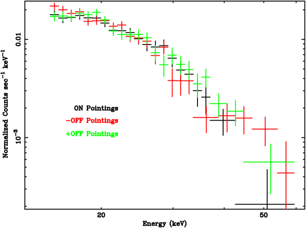
We obtained three difference spectra: for the ON–source pointings (2350 ks of exposure time), for the OFF–source pointings (800 ks) and for the OFF–source pointings (881 ks). They are shown in Fig. 3. As can be seen, all are consistent with each other within their uncertainties, as also confirmed with a run test (see, e.g., Bendat & Piersol 1971). The small observed deviations from each other give an indication of the systematic errors made in the estimate of the difference . However, the results from the offset and ON–source pointings agree within the statistical errors. On the basis of these results, for the derivation of the CXB intensity we used the sum which is well determined up to 50 keV (see Fig. 4).
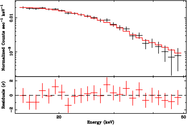
When is fit with a pl model, we find an unacceptable (= 37.4/23) in the 15–50 keV band, with a probability of 2.5% that this high value is due to chance. Instead, in the 20–50 keV band, an acceptable value (= 15.5/16) is found with a best fit pl photon index at 90% confidence level of , much higher than that of the CXB (see Table The cosmic X–ray background and the population of the most heavily obscured AGNs). Both results are expected if does give the difference spectrum between the CXB and the albedo from the dark Earth, with the first result mainly due to the presence of a low energy cutoff in the albedo spectrum (see Appendix B.1). The high also unequivocally shows that the albedo spectrum, above its cutoff, is harder than that of the CXB. Thus, in the 15 to 50 keV band, we fit with the difference of two model spectra, one to describe the unresolved CXB spectrum and the other to describe the albedo radiation spectrum.
For the albedo model spectrum we used a photo-electrically absorbed power–law photons cm-2 s-1 keV-1 sr-1, where is the normalization constant at 20 keV, is the air absorption coefficient in units of cm2/g, and is the atmospheric depth that describes the well known cutoff in the albedo spectrum at keV (see Appendix B.1). To describe the albedo low–energy cutoff, we developed an atmospheric absorption model within the XSPEC software package (Arnaud 1996), that we adopted for our model fitting. The model makes use of a grid of values of air mass X–ray attenuation coefficients as a function of the photon energy (Hubbell & Seltzer 1996). To model the CXB spectrum we assumed the CXB spectral shape obtained with HEAO–1 A2A4 (G99). Thus we used as input models a cutoffpl and a pl which, in the 15–50 keV interval, still gives a good description of this shape.
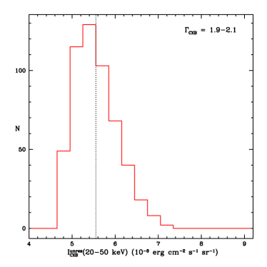
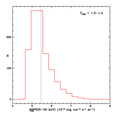
In order to better constrain the CXB spectral parameters, the fit of to the data was not performed by leaving free to vary all the model s parameters. In return, different fits were performed, each one with different set of values of the parameters frozen in the fits. These parameters were: the CXB photon index (when it was not left free to vary see Tab. 2), the atmospheric depth and the albedo pl photon index . The allowed ranges of were from 1.9 to 2.1 for the pl and from 1.2 to 1.4 interval for the cutoffpl, the allowed range of (in units of g cm-2) was from 1.4 to 6 and that of was from 1.3 to 2.0. Only the cutoff energy was always frozen to the value of 41.13 keV found with HEAO–1 (see Table The cosmic X–ray background and the population of the most heavily obscured AGNs), given that in our energy band (15–50 keV) the fits were insensitive to . These ranges include the values obtained in past measurements and take into account the fact that the albedo mean slope is harder than that of the CXB, as previously discussed. In this way the entire parameter space was explored. By uniformly subdividing the allowed ranges of , and in a certain number of subintervals, we obtained a grid of best fit values of those parameters that were left free to vary in the fits 111In all tables, those parameters that were frozen in the fits are shown in square brackets.. From this grid we have derived the frequency distribution of one of the most important quantities that characterize our CXB estimate, i.e., the 20–50 keV integrated intensity of the unresolved CXB 222We adopt this energy band given that it is common to all high energy X–ray experiments quoted in Table The cosmic X–ray background and the population of the most heavily obscured AGNs and Table The cosmic X–ray background and the population of the most heavily obscured AGNs.. In Fig. 5 we show this distribution, for both a pl and cutoffpl CXB model. It was obtained by performing 1200 trials (20 steps for , 20 for and 3 for ), and accepting only those spectral solutions (532 in the case of the pl, 1091 in the case of the cutoffpl) for which the pl photon index of the reconstructed spectrum in the 20–50 keV band is in the range 2.9–3.5, consistently with the observed slope of . (Without this constraint the peak of the distribution occurs at slightly lower values of .) We verified that the moments of this distribution are independent of the number of chosen steps.
As can be seen, the frequency distribution of is well peaked (also the frequency distribution of the and normalizations and of show a similar shape), with a mean value slightly higher than that at the maximum of the distribution (see Fig. 5). We have exploited this distribution to better constrain the range of the parameter values that were frozen in the single fits. Having adopted the maximum likelihood method (Janossy 1965) for the best estimate of the model parameters, we considered as best fit parameter values, reported in Table 2, those that, in the narrow flat top region of the frequency distribution around the mean value, give the minimum . In Fig. 4 we show the best fitting curve to and the corresponding residuals in the case of a pl as input model for the unresolved CXB, and dark Earth albedo spectral parameters frozen at the values shown in Table 2.
Using the frequency distributions, we also derived the upper limit to the unresolved CXB estimate finding that, independently of the CXB input model, 90% of the data points have erg cm-2 s-1 sr-1. We assume this value as upper limit to our estimate of the unresolved CXB. We notice that, by increasing the range of the CXB photon index values to 1.8–2.2 for the pl, and to 1.1–1.5 for cutoffpl, we find similar distributions with a mean at slightly lower intensity values but with upper limit almost unchanged with respect to that given above.
In Appendix B.2 we report and discuss the obtained results on the terrestrial albedo from the dark Earth. For a comparison of the CXB spectrum with the albedo spectrum see Fig. 8.
4 The total (resolved plus unresolved) CXB
Exploiting the PDS pointings, we also performed an estimate of the contribution of resolved sources to the 15–50 keV integrated CXB intensity. This estimate could not be done using the ON-source pointings of the PDS, given that most of them were pointed observations of specific targets by the BeppoSAX Narrow Field Instruments LECS, MECS, HPGSPC, and PDS. However, 33 of the PDS OFF–source fields, that were excluded from the data set for the unresolved CXB intensity determination (see Sect. 3.2), showed significant count excesses (2.5–7), consistent with the presence of serendipitous X–ray sources. The spectra of these excesses, when fit with a pl model, gave a weighted mean value of their photon indices equal to , while their intensity gave a 15–100 keV energy flux in the range (1.4–20) erg cm-2 s-1. A search of their counterparts is now in progress. Their contribution increases the CXB intensity by 4.7%. Adding the contribution of brighter sources (see, e.g., Krivonos et al. 2005) does not significantly change this figure.
Taking into account these results, in Table The cosmic X–ray background and the population of the most heavily obscured AGNs we report, for each of the used input models, the normalization of the total CXB (unresolved plus resolved) spectrum, while in Fig. 6 we show, for the pl and cutoffpl models, the best fit spectrum of the total CXB. In Table The cosmic X–ray background and the population of the most heavily obscured AGNs and Fig. 6 we also compare our measurement with the past results.
5 Discussion
It is apparent from Fig. 6 and Table The cosmic X–ray background and the population of the most heavily obscured AGNs that our best fit is in excellent agreement with that obtained with HEAO–1 A2 (M80), and slightly lower (from 3 to 10%, depending on the input model) than that quoted by G99. (As discussed in Section 2, the use of our flux scale calibration is more realistic; had we used the scale calibration given by Jung (1989) for HEAO–1 A4, our best fit would range from 0.95 to 1.03 times the corresponding value derived from G99.) The best fit value of the maximum CXB flux density is obtained in the 26–28 keV band and ranges from 39.4 to 40.2 keV (cm2 s sr)-1 depending on the model assumed, with a statistical uncertainty in the centroid of keV (cm2 s sr)-1 at 90% confidence level for a single interesting parameter.
We have also evaluated the upper limit to the CXB intensity that can be marginally accommodated by our data, by exploring the space of all the parameters involved in the fits. We find that, taking also into account the contribution of the resolved sources, independently of the CXB model, in 90% of this multi-parameter space the is lower than erg cm-2 s-1 sr-1, which is 12% higher than the best fit CXB intensity value quoted by G99 and 21% higher than that quoted by M80 (see Table The cosmic X–ray background and the population of the most heavily obscured AGNs).
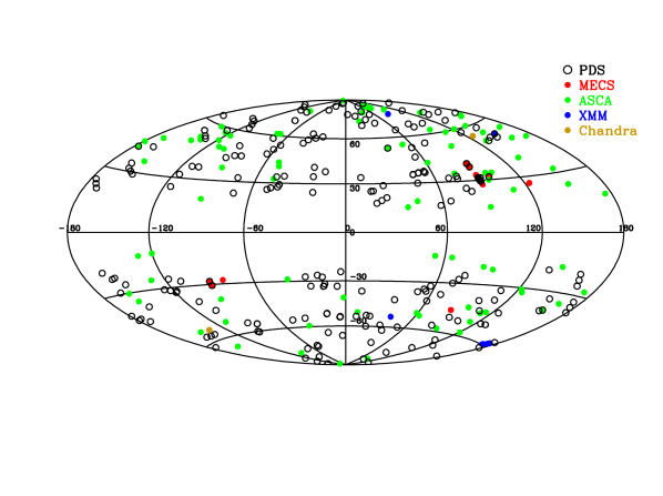
Even this upper limit disagrees with the extrapolation to higher energies of the low energy (10 keV) CXB estimates obtained with the focusing telescopes aboard BeppoSAX (Vecchi et al. 1999), XMM–Newton (Lumb et al. 2002; De Luca & Molendi 2004), and Chandra (Hickox & Markevitch 2006), but it is consistent with those obtained with ASCA and RXTE. Thus, if we exclude a change in the CXB spectral shape derived with HEAO–1, our results raise the issue about the origin of the highest CXB intensities being quoted at lower energies. Differences in the flux scale calibration do not appear to be the origin of these discrepancies, as discussed in Section 2. One may think that part of the discrepant results could be due to the amount of sky solid angle surveyed, which is very large in the case of HEAO–1 and BeppoSAX PDS, and very small in the case of BeppoSAX MECS, XMM–Newton and Chandra (see Fig. 7), although, as also discussed by Barcons et al. (2000), this would imply that the sky regions surveyed by these telescopes are systematically brighter than the average sky sampled with HEAO–1 and BeppoSAX PDS. Another possible origin of the highest 2–10 keV CXB estimates could be due to systematic errors in the response function used for the diffuse emission (e.g., an underestimate of the stray light). For instance, in the case of MECS this function could be well tested and cross-calibrated with the PDS only for point-like sources.
Independently of the CXB intensity issue at lower energies, our observational findings bear at least two important astrophysical consequences. Firstly, they provide a robust estimate of the accretion driven power integrated over cosmic time, including that produced by the most obscured AGNs. The AGN synthesis models, tuned to attain the PDS CXB level and to account for the hard X–ray spectral shape (La Franca et al. 2005; Gilli et al. 2006), predict that at the bright fluxes ( erg cm-2 s-1) reachable by the PDS observations and by coded mask instruments like INTEGRAL IBIS and Swift BAT, the detectable fraction of extremely obscured AGNs (Compton thick, cm-2) is 10%, and it increases to 20–25% at the fluxes reachable by focusing telescopes (e.g. Ferrando et al. 2006). It should be noted that the highest CXB intensities claimed at low energies (Vecchi et al. 1999; De Luca & Molendi 2004; Hickox & Markevitch 2006, see Table The cosmic X–ray background and the population of the most heavily obscured AGNs) would entail a much larger number (a factor 2–3) of Compton thick AGNs (Gilli et al. 2006), a prediction barely consistent with the present observational evidence. Our result implies a present black hole mass density of M⊙ Mpc-3, using an admittedly uncertain bolometric correction of 30 for the 15–50 keV band and an efficiency of 0.1 in converting gravitational into radiation energy. This corresponds to a fraction of of all baryons being locked into the supermassive black holes, using a cosmic baryon density of g cm-3 in agreement with the “concordance” cosmology model.
Secondly, under the assumption that the HEAO–1 spectral shape (G99) applies down to 2 keV, we find that the summed contribution of the observed X–ray source counts in the 2–10 keV band (Moretti et al. 2003) exceeds the PDS CXB best fit level by 11%. This apparent contradiction vanishes if one takes into account the above discussed upper limit in the PDS CXB intensity level and the error (7%) associated with the source count evaluation (Moretti et al. 2003). As a consequence, our measurement suggests that it is quite possible that almost all the CXB in the 3–8 keV band has already been resolved into sources down to the faintest fluxes of the Chandra deep fields. Any substantial contribution to the CXB from other classes of sources and diffuse WHIM should be confined at photon energies below 3 keV, as it has already been indicated in the case of star forming galaxies (Ranalli et al. 2003).
Appendix A The solid angle of the PDS instrument
The solid angle of the PDS is derived from the Geometric Factor of the telescope defined as (Peterson et al. 1973; Horstman et al. 1975)
| (A1) |
where is the exposed detector geometric area through the collimators at an offset angle , and is the solid angle of the instrument Field of View (FOV). The expression of , for an hexagonal collimator like that of the PDS, can be found in Horstman et al. (1975) and is given by
| (A2) |
where is the ON–axis geometric area through the collimator (640 cm2), is the diameter of the circumscribed circle to the hexagonal collimator cells, and is collimator height. The ratio is related to the minimum FWHM of the angular response of the PDS through the relation
| (A3) |
Using the value of derived from the offset Crab observations, we obtain a value of cm2 sr and, dividing by cm2, we find the telescope solid angle sr.
Appendix B The albedo spectrum
B.1 The past measurements
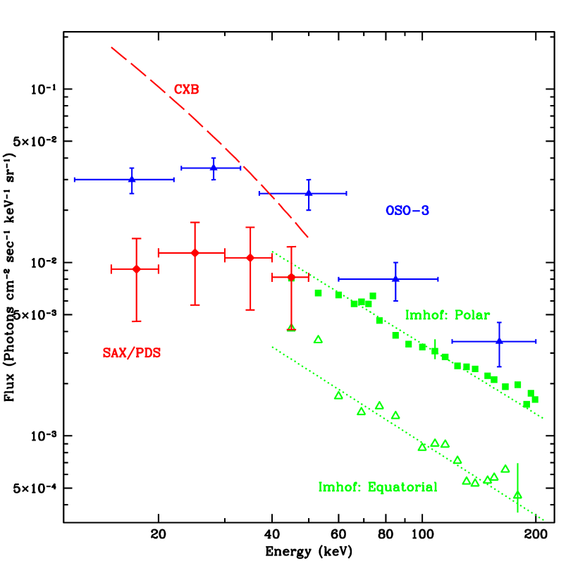
The terrestrial gamma–ray albedo radiation is mainly the result of the interactions with the upper atmosphere of the Cosmic Rays and, at X–ray energies, of the CXB and of the discrete X–ray source radiation (Compton reflection). It was investigated since the late 1960s (see Peterson 1975, for a review). Most of the properties of the atmospheric gamma–rays were obtained with balloon experiments, mainly launched from Palestine (Texas, USA). Empirical models of the atmospheric gamma–ray emission, based on observational results, were worked out by various authors (Peterson 1975; Ling 1975; Dean et al. 1989). From these observations, it can be seen that the gamma–ray emission properties depend on various parameters, like the geomagnetic latitude, the energy band, the direction of emission (downward, upward) and the altitude from the Earth. The atmospheric radiation measured by a satellite depends on these parameters, but, unlike the radiation observed by a balloon experiment, a satellite observes only the radiation emerging from the top of the atmosphere (albedo radiation). Thus its spectral properties, specially at low energies (10 keV), are expected to be different from those observed inside the atmosphere. Measurements of the X–ray albedo radiation are reported in Schwartz & Peterson (1974) for photon energies in the 10–300 keV band, and in Imhof et al. (1976) above 40 keV, while for energies higher than 150 keV see, e.g., Letaw et al. (1986) and Dean et al. (1989).
The albedo spectrum of Schwartz & Peterson (1974), which was obtained with a 0.5 cm scintillator detector and a wide FOV ( at zero response) aboard the OSO–3 satellite in a nearly circular orbit at an inclination of 33∘ and an altitude of 550 km (Schwartz et al. 1970), above 40 keV is consistent with a pl (see Fig. 8), while below 40 keV it shows a flattening with a definitive low energy cutoff below 30 keV. This cutoff is also observed with balloon experiments (Peterson et al. 1973; Peterson 1975; Schwartz & Peterson 1974) and it is attributed to self-absorption of the radiation collectively emitted from different atmospheric layers. The pl model above 40 keV is confirmed by the albedo spectrum measured with a 50 cm3 Ge(Li) cooled detector with a wide FOV as well ( at zero response) aboard the low–altitude polar–orbiting satellite 1972–076B (see Fig. 8; Imhof et al. 1976).
Following Schwartz (1969), the best fit to the 10 keV albedo spectrum measured with OSO–3 is obtained with a photo-electrically absorbed pl photons cm-2 s-1 keV-1 sr-1, with photon index , and atmospheric thickness g/cm2 (at 90% confidence level). In the case of the polar–orbiting satellite, Imhof et al. (1976) found that above 40 keV the photon spectrum is consistent with a pl with index ranging from 1.34 to 1.39, depending on the latitude scanned.
On the basis of these observations, we have assumed a photo-electrically absorbed pl as a model spectrum for the albedo radiation from the dark Earth.
B.2 Our results
In addition to the parameter values reported in Table 2, we show in Fig. 8 the derived spectrum of the terrestrial albedo from the dark Earth, compared with that of the CXB. As can be seen, the derived albedo spectrum is located between the OSO-3 results and the albedo spectrum derived by Imhof et al. (1976), with a 20–50 keV integrated intensity of erg cm-2 s-1 sr-1. It should be noticed that the intensity of the albedo radiation depends on the CR flux hitting the Earth, and thus on magnetic latitude. Given that in different Earth pointings we pointed to the Earth along generally different directions and thus to different magnetic latitudes, the derived spectrum is latitude averaged, as partially done also in the case of the OSO–3 and 1972–076B satellites due to their wide FOVs. We also notice that at different latitudes we do not observe the upward albedo, but the albedo emerging at different zenith angles . However, as discussed by Ling (1975), the atmospheric spectrum at low energies is expected to be not strongly anisotropic with .
References
- Arnaud (1996) Arnaud, K. A. 1996, ASP Conf. Series, 101, 17
- Ballantyne et al. (2006) Ballantyne, D. R., Everett, J. E., & Murray, N. 2006, ApJ, 639, 740
- Barcons et al. (2000) Barcons, X., Mateos, S., & Ceballos, M. T. 2000, MNRAS, 316, L13
- Bartlett (1994) Bartlett, L. M. 1994, PhD thesis, NASA/Goddard Space Flight Center
- Bendat & Piersol (1971) Bendat, J. S. & Piersol, A. G. 1971, Random data: Analysis and Measurement Procedures (Wiley–Interscience)
- Boella et al. (1997a) Boella, G., Butler, R. C., Perola, G. C., Piro, L., Scarsi, L., & Bleeker, J. A. M. 1997a, A&AS, 122, 299
- Boella et al. (1997b) Boella, G., Chiappetti, L., Conti, G., Cusumano, G., del Sordo, S., La Rosa, G., Maccarone, M. C., Mineo, T., Molendi, S., Re, S., Sacco, B., & Tripiciano, M. 1997b, A&AS, 122, 327
- Churazov et al. (2006) Churazov, E., Sunyaev, R., Revnivtsev, M., Sazonov, S., Molkov, S., Grebenev, S., Winkler, C., Parmar, A., Bazzano, A., Falanga, M., Gros, A., Lebrun, F., Natalucci, L., Ubertini, P., Roques, J. ., Bouchet, L., Jourdain, E., Knoedlseder, J., Diehl, R., Budtz-Jorgensen, C., Brandt, S., Lund, N., Westergaard, N. J., Neronov, A., Turler, M., Chernyakova, M., Walter, R., Produit, N., Mowlavi, N., Mas-Hesse, J. M., Domingo, A., Gehrels, N., Kuulkers, E., Kretschmar, P., & Schmidt, M. 2006, A&A, submitted (astro-ph/0608250)
- Comastri (2004) Comastri, A. 2004, in Multiwavelength AGN Surveys, ed. R. Mujica & R. Maiolino (Singapore: World Scientific Publishing Company), 323
- Comastri et al. (1995) Comastri, A., Setti, G., Zamorani, G., & Hasinger, G. 1995, A&A, 296, 1
- De Luca & Molendi (2004) De Luca, A. & Molendi, S. 2004, A&A, 419, 837
- Dean et al. (1989) Dean, A. J., Fan, L., Byard, K., Goldwurm, A., & Hall, C. J. 1989, A&A, 219, 358
- Ferrando et al. (2006) Ferrando, P., Arnaud, M., Briel, U., Citterio, O., Clédassou, R., Duchon, P., Fiore, F., Giommi, P., Goldwurm, A., Hasinger, G., Kendziorra, E., Laurent, P., Lebrun, F., Limousin, O., Malaguti, G., Mereghetti, S., Micela, G., Pareschi, G., Rio, Y., Roques, J. P., Strüder, L., & Tagliaferri, G. 2006, in Space Telescopes and Instrumentation II: Ultraviolet to Gamma Ray. Proceedings of the SPIE, Volume 6266, ed. M. Turner & G. Hasinger, 11
- Frontera et al. (1997a) Frontera, F., Costa, E., Dal Fiume, D., Feroci, M., Nicastro, L., Orlandini, M., Palazzi, E., & Zavattini, G. 1997a, Proc. SPIE, 3114, 206
- Frontera et al. (1997b) Frontera, F., Costa, E., dal Fiume, D., Feroci, M., Nicastro, L., Orlandini, M., Palazzi, E., & Zavattini, G. 1997b, A&AS, 122, 357
- Gendreau et al. (1995) Gendreau, K. C., Mushotzky, R., Fabian, A. C., Holt, S. S., Kii, T., Serlemitsos, P. J., Ogasaka, Y., Tanaka, Y., Bautz, M. W., Fukazawa, Y., Ishisaki, Y., Kohmura, Y., Makishima, K., Tashiro, M., Tsusaka, Y., Kunieda, H., Ricker, G. R., & Vanderspek, R. K. 1995, PASJ, 47, L5
- Georgantopoulos et al. (1996) Georgantopoulos, I., Stewart, G. C., Shanks, T., Boyle, B. J., & Griffiths, R. E. 1996, MNRAS, 280, 276
- Gilli (2004) Gilli, R. 2004, Adv. Space Res., 34, 2470
- Gilli et al. (2006) Gilli, R., Comastri, A., & Hasinger, G. 2006, A&A, in press (astro-ph/0610939)
- Gruber (1992) Gruber, D. E. 1992, in The X–ray Background, ed. X. Barcons & A. Fabian ((Cambridge: Cambridge University Press)), 44
- Gruber et al. (1999) Gruber, D. E., Matteson, J. L., Peterson, L. E., & Jung, G. V. 1999, ApJ, 520, 124
- Hickox & Markevitch (2006) Hickox, R. C. & Markevitch, M. 2006, ApJ, 645, 95
- Hopkins et al. (2006) Hopkins, P. F., Hernquist, L., Cox, T. J., Di Matteo, T., Robertson, B., & Springel, V. 2006, ApJS, 163, 1
- Horstman et al. (1975) Horstman, H. M., Cavallo, G., & Moretti-Horstman, E. 1975, Rivista Nuovo Cimento, 5, 255
- Hubbell & Seltzer (1996) Hubbell, J. H. & Seltzer, S. M. 1996, available online at http://physics.nist.gov/PhysRefData/XrayMassCoef/cover.html
- Imhof et al. (1976) Imhof, W. L., Nakano, G. H., & Reagan, J. B. 1976, J. Geophys. Res., 81, 2835
- Jahoda & et al. (2006) Jahoda, K. & et al. 2006, in preparation (available online at http://lheawww.gsfc.nasa.gov/users/keith/a2_cxb_15dec2005.pdf)
- Janossy (1965) Janossy, M. 1965, Theory and practice of the evaluation of measurements (Clarendon Press, London)
- Jung (1989) Jung, G. V. 1989, ApJ, 338, 972
- Kinzer et al. (1978) Kinzer, R. L., Johnson, W. N., & Kurfess, J. D. 1978, ApJ, 222, 370
- Kinzer et al. (1997) Kinzer, R. L., Jung, G. V., Gruber, D. E., Matteson, J. L., & Peterson, L. E. 1997, ApJ, 475, 361
- Kirsch et al. (2005) Kirsch, M. G., Briel, U. G., Burrows, D., Campana, S., Cusumano, G., Ebisawa, K., Freyberg, M. J., Guainazzi, M., Haberl, F., Jahoda, K., Kaastra, J., Kretschmar, P., Larsson, S., Lubinski, P., Mori, K., Plucinsky, P., Pollock, A. M., Rothschild, R., Sembay, S., Wilms, J., & Yamamoto, M. 2005, in Proceedings of the SPIE, Volume 5898, ed. O. H. W. Siegmund, 22
- Krivonos et al. (2005) Krivonos, R., Vikhlinin, A., Churazov, E., Lutovinov, A., Molkov, S., & Sunyaev, R. 2005, ApJ, 625, 89
- Kuntz et al. (2001) Kuntz, K. D., Snowden, S. L., & Mushotzky, R. F. 2001, ApJ, 548, L119
- Kushino et al. (2002) Kushino, A., Ishisaki, Y., Morita, U., Yamasaki, N. Y., Ishida, M., Ohashi, T., & Ueda, Y. 2002, PASJ, 54, 327
- La Franca et al. (2005) La Franca, F., Fiore, F., Comastri, A., Perola, G. C., Sacchi, N., Brusa, M., Cocchia, F., Feruglio, C., Matt, G., Vignali, C., Carangelo, N., Ciliegi, P., Lamastra, A., Maiolino, R., Mignoli, M., Molendi, S., & Puccetti, S. 2005, ApJ, 635, 864
- Letaw et al. (1986) Letaw, J. R., Share, G. H., Kinzer, R. L., Silberberg, R., & Chupp, E. L. 1986, Adv. Space Res., 6, 133
- Ling (1975) Ling, J. C. 1975, J. Geophys. Res., 80, 3241
- Lumb et al. (2002) Lumb, D. H., Warwick, R. S., Page, M., & De Luca, A. 2002, A&A, 389, 93
- Marshall et al. (1980) Marshall, F. E., Boldt, E. A., Holt, S. S., Miller, R. B., Mushotzky, R. F., Rose, L. A., Rothschild, R. E., & Serlemitsos, P. J. 1980, ApJ, 235, 4
- McCammon et al. (1983) McCammon, D., Burrows, D. N., Sanders, W. T., & Kraushaar, W. L. 1983, ApJ, 269, 107
- Moretti et al. (2003) Moretti, A., Campana, S., Lazzati, D., & Tagliaferri, G. 2003, ApJ, 588, 696
- Peterson et al. (1973) Peterson, J. L., Schwartz, D. A., & Ling, J. C. 1973, J. Geophys. Res., 78, 7942
- Peterson (1975) Peterson, L. E. 1975, ARA&A, 13, 423
- Ranalli et al. (2003) Ranalli, P., Comastri, A., & Setti, G. 2003, A&A, 399, 39
- Revnivtsev et al. (2005) Revnivtsev, M., Gilfanov, M., Jahoda, K., & Sunyaev, R. 2005, A&A, 444, 381
- Revnivtsev et al. (2003) Revnivtsev, M., Gilfanov, M., Sunyaev, R., Jahoda, K., & Markwardt, C. 2003, A&A, 411, 329
- Schwartz (1969) Schwartz, D. A. 1969, PhD thesis, University of California at San Diego
- Schwartz et al. (1970) Schwartz, D. A., Hudson, H. S., & Peterson, L. E. 1970, ApJ, 162, 431
- Schwartz & Peterson (1974) Schwartz, D. A. & Peterson, L. E. 1974, ApJ, 190, 297
- Setti & Woltjer (1989) Setti, G. & Woltjer, L. 1989, A&A, 224, L21
- Toor & Seward (1974) Toor, A. & Seward, F. D. 1974, AJ, 79, 995
- Ueda et al. (2003) Ueda, Y., Akiyama, M., Ohta, K., & Miyaji, T. 2003, ApJ, 598, 886
- Vecchi et al. (1999) Vecchi, A., Molendi, S., Guainazzi, M., Fiore, F., & Parmar, A. N. 1999, A&A, 349, L73
- Willingale et al. (2001) Willingale, R., Aschenbach, B., Griffiths, R. G., Sembay, S., Warwick, R. S., Becker, W., Abbey, A. F., & Bonnet-Bidaud, J.-M. 2001, A&A, 365, L212
- Worsley et al. (2006) Worsley, M. A., Fabian, A. C., Bauer, F. E., Alexander, D. M., Brandt, W. N., & Lehmer, B. D. 2006, MNRAS, 368, 1735
- Worsley et al. (2005) Worsley, M. A., Fabian, A. C., Bauer, F. E., Alexander, D. M., Hasinger, G., Mateos, S., Brunner, H., Brandt, W. N., & Schneider, D. P. 2005, MNRAS, 357, 1281
- Zombeck (1990) Zombeck, M. V. 1990, Handbook of Space Astronomy and Astrophysics (Cambridge University Press)
| Instrument | Ref. | Energy band | Model | or | |||
|---|---|---|---|---|---|---|---|
| (keV) | (keV) | ||||||
| Composite | (1) | 1–20 | PLa | – | 1.07 | – | |
| Composite | (1) | 20–200 | PLa | – | – | ||
| Composite | (2) | 20–165 | PLa | – | – | ||
| HEAO–1/A2 | (3) | 3–50 | BREMSSb | – | [40] | ||
| HEAO–1/A2 | (4) | 2–10 | PLa | [1.4] | – | – | |
| HEAO–1/A2 | (5) | 2–10 | PLa | [1.558]c | – | – | |
| HEAO–1/A2A4 | (6,7) | 3–60 | CUTOFFPLd | 1 | 1 | ||
| Rocket | (8) | 2–6 | PLa | [1.4] | – | – | |
| ROSAT/PSPC | (9) | 0.7–2.4 | PLa | – | – | ||
| SAX/MECS | (10) | 1–8 | PLa | – | – | ||
| ASCA/SIS | (11) | 1–7 | PLa | – | – | ||
| ASCA/GIS | (12) | 1–10 | PLa | [1.4] | – | – | |
| XMM/EPIC-MOS/PN | (13) | 2–8 | PLa | – | – | ||
| RXTE/PCA | (14) | 3–20 | PLa | – | – | ||
| XMM/EPIC-MOS | (15) | 2-8 | PLa | – | – | ||
| Chandra/ACIS-I | (16) | 2–8 | PLa | [1.4] | – | – |
Note. — The reported energy band gives the interval in which the CXB spectrum and its model parameters have been determined. gives the ratio between the 2–10 keV intensity estimated from the reported parameters and that obtained with HEAO–1 ( erg cm-2 s-1 sr-1). Likewise gives the ratio between the estimated 20–50 keV intensity and that obtained with HEAO–1( erg cm-2 s-1 sr-1). In square parenthesis the parameter values that were kept constant by the quoted authors. Uncertainties are 1 errors for a single parameter. Where not reported, the uncertainties are very small or are not reported in the quoted papers.
References. — (1) Horstman et al. (1975); (2) Kinzer et al. (1978); (3) M80; (4) Revnivtsev et al. (2005); (5)Jahoda & et al. (2006); (6) Gruber (1992); (7) G99; (8) McCammon et al. (1983); (9) Georgantopoulos et al. (1996); (10) Vecchi et al. (1999); (11) Gendreau et al. (1995); (12) Kushino et al. (2002); (13) Lumb et al. (2002); (14) Revnivtsev et al. (2003); (15) De Luca & Molendi (2004); (16) Hickox & Markevitch (2006).
| CXB model | f | |||||||
|---|---|---|---|---|---|---|---|---|
| Power-lawa | [1.98] | – | [1.38] | [1.91] | 9.43/23 | |||
| Cutoff power-lawb | [1.4] | [41.13] | [1.53] | [2.42] | 9.2/23 | |||
| Cutoff power-lawb | [41.13] | [1.3] | [1.4] | 9.0/22 | ||||
| Cutoff power-lawb | [1.29] | [41.13] | [2.0] | [4.98] | 9.2/23 |
Note. — is the unresolved CXB normalization at 20 keV, while gives the intensity of the dark Earth albedo at 20 keV. The last column gives the unresolved 20–50 keV integrated intensity. The parameters that were frozen in the fits are shown in square brackets. The quoted uncertainties are errors at 90% confidence level for a single parameter.
| Experiment | Ref. | Energy band | Model | or | f | |||
|---|---|---|---|---|---|---|---|---|
| (keV) | (keV) | |||||||
| Composite | (1) | 20–200 | PLa | – | – | |||
| Balloon | (2) | 20–165 | PLa | – | – | |||
| HEAO–1/A2 | (3) | 3–50 | BREMSSb | – | [40] | – | ||
| HEAO–1/A2+A4 | (4) | 3–60 | CUTOFFPLc | [1.29] | [41.13] | |||
| SAX/PDS | this paper | 15–50 | PLd | [1.98] | – | |||
| SAX/PDS | this paper | 15–50 | CUTOFFPLe | [1.4] | [41.13] | |||
| SAX/PDS | this paper | 15–50 | CUTOFFPLe | [41.13] | ||||
| SAX/PDS | this paper | 15–50 | CUTOFFPLe | [1.29] | [41.13] |
Note. — For each model, the energy band of the CXB spectral determination, the parameters of its photon spectrum and the 20–50 keV energy flux per steradian are reported. For flux scale calibration purposes, when available, also the 20–50 Crab flux predicted from the single experiments is reported. Uncertainties are 1 errors. Parameters in square parenthesis are those kept fixed in the single fits.