An improved model for the formation times of dark matter haloes

Abstract

A dark matter halo is said to have formed when at least half its mass hass been assembled into a single progenitor. With this definition, it is possible to derive a simple but useful analytic estimate of the distribution of halo formation times. The standard estimate of this distribution depends on the shape of the conditional mass function—the distribution of progenitor masses of a halo as a function of time. If the spherical collapse model is used to estimate the progenitor mass function, then the formation times one infers systematically underestimate those seen in numerical simulations of hierarchical gravitational clustering. We provide estimates of halo formation which may be related to an ellipsoidal collapse model. These estimates provide a substantially better description of the simulations. We also provide an alternative derivation of the formation time distribution which is based on the assumption that haloes increase their mass through binary mergers only. Our results are useful for models which relate halo structure to halo formation.

1 Introduction

Large samples of galaxy clusters selected in the optical (Miller et al., 2005; McKay et al., 2005) and other bands (ACT, SPT) will soon be available. These cluster catalogs will be used to constrain cosmological parameters. The tightness of such constraints depends on the accuracy with which the masses of the clusters can be determined from observed properties. These properties are expected to depend on the formation histories of the clusters. Models of cluster formation identify clusters with massive dark matter halos, so understanding cluster formation requires an understanding of dark halo formation.

There is also some interest in using the distribution of galaxy velocity dispersions (Sheth et al., 2003) to constrain cosmological parameters (Newman & Davis, 2002). The velocity dispersion of a galaxy is expected to be related to the concentration of the halo which surrounds it, and this concentration is expected to be influenced by the formation history of the halo (Tormen, 1998; Bullock et al., 2001; Wechsler et al., 2002). Hence, this program also benefits from understanding the formation histories of dark matter halos.

In hierarchical models, the formation histories of dark matter halos are expected to depend strongly on halo mass—massive halos are expected to have formed more recently (Press & Schechter, 1974). But quantifying this tendency requires a more precise definition of what one means by the ‘formation time’. Lacey & Cole (1993) provided a simple definition—it is the earliest time when a single progenitor halo contains half the final mass. For this definition, they showed how to estimate the distribution of halo formation times. Sheth & Tormen (2004) provide associated expressions for the joint distribution of formation time and the mass at formation. This estimate depends on the distribution of progenitor masses at earlier times, and Lacey & Cole used the assumption that halos form from a spherical collapse to estimate this conditional mass function. However, a model based on ellipsoidal collapse provides a more accurate description of the abundances of dark halos (Sheth, Mo & Tormen, 2001) and of their progenitors (Sheth & Tormen, 2002). Hence, one expects to find that the ellipsoidal collapse model also provides a better description of halo formation. The primary goal of the present work is to study if this is indeed the case.

Section 2 reviews Lacey & Cole’s argument, and describes how we estimate the ellipsoidal collapse based progenitor mass functions. Explicit formulae are provided in Appendix A. Section 3 compares the model predictions for halo formation with measurements in simulations of hierarchical gravitational clustering. The simulations, and how we estimate halo formation times in them, are described in Section 3.1. Sections 3.2 and 3.3 show that the spherical collapse model predicts lower formation redshifts than are seen in the simulations, particularly at low masses. Insertion of ellipsoidal collapse based expressions in Lacey & Cole’s formalism provides substantially increased accuracy. However, the agreement is not perfect—although the ellipsoidal collapse based expressions provide a good description of how the median formation redshift decreases with halo mass, it predicts formation time distributions which are broader than seen in the simulations. A final section summarizes our results and discusses possible reasons for the discrepancy.

There is some confusion in the literature about the relation between halo formation as defined by Lacey & Cole (1993), and a quantity which arises in binary merger models of hierarchical clustering. The relation between this other quantity and the one defined by Lacey & Cole is clarified in Appendix B.

2 The formation time distribution

Following Lacey & Cole (1993), we will define the formation time of a halo as the earliest time that at least half of its mass has been assembled into a single progenitor.

2.1 Relation to the progenitor mass function

Consider an ensemble of halos of mass $M$ at time $T$, and let $N(m,t|M,T)$ denote the average number of progenitors of these halos that have mass $m<M$ at time $t<T$. Since a halo can have at most one progenitor of mass $m>M/2$, the fraction of halos which have a progenitor of mass $m>M/2$ at time $t$ is

$$\int_{M/2}^{M}{\rm d}m\,N(m,t|M,T).$$

But, because they have a progenitor of mass $m>M/2$, these halos are also the ones which formed at some $t_{\rm f}<t$. Hence,

$$\int_{0}^{t_{\rm f}}{\rm d}t\,p(t|M,T)=\int_{M/2}^{M}{\rm d}m\,N(m,t_{\rm f}|M,T),$$ (1)

where $p(t|M,T)$ denotes the probability that a halo of mass $M$ at $T$ formed at time $t$. Differentiating with respect to $t_{\rm f}$ yields

$$p(t_{\rm f}|M,T) = \frac{\rm d}{{\rm d}t_{\rm f}}\int_{M/2}^{M}{\rm d}m\,N(m,t_{\rm f}|M,T)$$ (2)

$$= \int_{M/2}^{M}{\rm d}m\,\frac{{\rm d}N(m,t_{\rm f}|M,T)}{{\rm d}t_{\rm f}}.$$ (3)

Evidently, the formation time distribution is closely related to the distribution of progenitor masses and its evolution. Different estimates of the progenitor mass function will result in different formation time distributions.

In what follows, we will estimate the distribution of halo formation times using equation (2). Thinking along the lines of equation (3) instead shows how $p(t_{\rm f}|M,T)$ can be related to quantities which arise naturally in binary merger models of hierarchical clustering. Appendix B provides details.

Lacey & Cole (1993) used estimates for $N(m,t|M,T)$ which were derived from a model in which halos form from a spherical collapse (Gunn & Gott, 1972; Press & Schechter, 1974). In this case, they showed that the distribution of formation times could be scaled to a universal form:

$$p(\omega)=2\omega\,{\rm erfc}(\omega/\sqrt{2})$$ (4)

where

$$\omega=\sqrt{q}\,{\delta_{\rm sc}(z_{\rm f})-\delta_{\rm sc}(z_{0})\over\sqrt{S(M/2)-S(M)}}$$ (5)

and $q=1$. Here $\delta_{\rm sc}(z)$ is the overdensity required for spherical collapse at $z$, and $S(M)$ is the variance in the linear fluctuation field when smoothed with a top-hat filter of scale $R=(3M/4\pi\bar{\rho})^{1/3}$, where $\bar{\rho}$ is the comoving density of the background. In essence, $\omega$ is simply a scaled time variable: in an Einstein de-Sitter background cosmology $\omega\propto(z_{\rm f}-z_{0})$, where the constant of proportionality depends on the final mass $M$.

Strictly speaking, this expression is valid for a white-noise power spectrum ($S(m)\propto m^{-1})$, but it has been found to provide a reasonable aproximation for more general power spectra as well. For this distribution, the median value of $\omega$ is $0.974$, and the associated cumulative distribution is

$$P(>\omega)=\sqrt{\frac{2}{\pi}}\,\omega\,\mathrm{e}^{-\omega^{2}/2}+(1-\omega^{2})\,\mathrm{erfc}\Big{(}\frac{\omega}{\sqrt{2}}\Big{)}\,.$$ (6)

However, recent work has shown that the spherical collapse model predicts fewer massive halos and more intermediate mass halos than are seen in simulations of hierarchical gravitational clustering (Sheth & Tormen, 1999). Models in which halos form from an ellipsoidal collapse may be more accurate (Sheth, Mo & Tormen, 2001). These models also provide a better description of the progenitor mass function (Sheth & Tormen, 2002). In what follows, we will show the effects of substituting the ellipsoidal collapse based expressions for $N(m,t|M,T)$ in equation (1). We will also show that simply taking values of $q$ smaller than one will make equation (6) a good fit to the formation redshift associated to the ellipsoidal collapse.

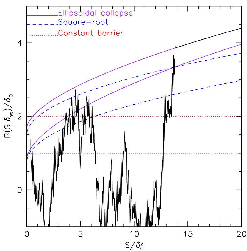
Figure 1: An example of a random walk and the three barrier shapes we consider in this paper. Here $\delta_{0}$ refers to the critical value associated with spherical collapse overdenisity at redshift $z_{0}$. The jagged line is a sample brownian walk absorbed by the barrier associated with ellipsoidal collapse (solid curve). Short-dashed curves show the square-root barriers which we use to approximate the ellipsoidal collapse barrier, and horizontal dotted lines show the constant barrier associated with spherical collapse. The upper set of barriers are associated with collapse at an earlier time.

2.2 Progenitor mass functions in the excursion set approach

We will use two approximations for the progenitor mass function. Both forms are derived from casting the ellipsoidal collapse model in the same language used for the spherical model—the excursion set formalism of Bond et al. (1991). In this formalism, halo abundances at a given time are associated with the first crossing distribution by Brownian motion random walks, of a barrier whose height decreases with time, and may in addition depend on how many steps the walk has taken. Figure 1 illustrates: it shows a walk which starts at some initial $S(M)$, and walks to the right, eventually crossing the barrier at some larger value of $S(m)>S(M)$. Here $S(m)$ is the variance in the initial fluctuation field when smoothed with a tophat filter of comoving scale $R=(3m/4\pi\bar{\rho})^{1/3}$, ($\bar{\rho}$ is the comoving background density), and the height of the walk represents the value of the initial density field when smoothed on scale $R$. In hierarchical models, $S(m)$ is a monotonically decreasing function of mass $m$. Hereafter we will use $\delta_{0}$ and $\delta_{1}$ to indicate the overdensity associated with the spherical collapse model respectively at redshift $z_{0}$ and $z_{1}$.

In the excursion set approach, the shape of the barrier, $B(S)$, depends on the collapse model. If the barrier is crossed on scale $S(m)$, then this indicates that the mass element on which the sphere is centered will be part of a collapsed object of mass $m$. Bond et al. used the fraction of walks which cross $B(S)$ at $S(m)$ as an estimate of the fraction of mass in halos of mass $m$: the parent halo mass function. Similarly, the fraction $f(s|S)$ of walks which start from some scale $S(M)$ and height $B(S)$ and first cross the barrier $B(s)$ at some $s>S$, can be used to provide an estimate of the progenitor mass function of $M$ halos:

$$N(m|M)\,{\rm d}m=\left(\frac{M}{m}\right)\,f(s|S)\,{\rm d}s$$ (7)

(note that $m<M$ because $s>S$). Thus, in the excursion set approach, the shape of $N(m|M)$ depends on how the shape of the barrier changes with mass—it is in this way that the collapse model affects the parent halo and progenitor mass functions.

The barrier shape is particularly simple for the spherical model: $B=\delta_{\rm sc}$ is the same constant for all values of $S$. Sheth, Mo & Tormen (2001) argued that the barrier associated with ellipsoidal collapse scales approximately as

$$B(S)=\sqrt{q}\delta_{\rm sc}\left\{1+\beta\left[{S(m)\over q\delta_{\rm sc}^{2}}\right]^{\gamma}\right\},$$ (8)

where $\delta_{\rm sc}$ is the value associated with complete collapse in the spherical model. Following Sheth et al., we set $\beta=0.5$, $\gamma=0.6$ and $q=0.707$; the values of the first two parameters are motivated by an analysis of the collapse of homogeneous ellipsoids, whereas the value of $q$ comes from requiring that the predicted halo abundances match those seen in simulations. The standard spherical model has $\beta=0$ and $q=1$; we will also show the predictions of this model if $\beta=0$ but $q=0.707$.

For general $\gamma$, exact analytic solutions to the first crossing distribution of barriers given by equation (8) are not available. For this reason, we have studied two analytic approximations which result from addressing the first crossing problem in two different ways. The first approach uses an analytic approximation to the first crossing distribution which Sheth & Tormen (2002) showed was reasonably accurate.

Our second approach is to substitute the ellipsoidal collapse barrier for one which is similar, but for which an exact analytic expression for the first crossing distribution is available. Specifically, when $\gamma=0.5$, then the barrier height increases with the square-root of $S$, and the first crossing distribution can be written as a sum of parabolic cylinder functions (Breiman 1966). In this approach, we approximate the progenitor mass function using an expression which would be exact for a square-root barrier, bearing in mind that the square-root barrier is an approximation to the ellipsoidal collapse dynamics. For this barrier shape, we set $\beta=0.5$ and $q=0.55$ since these choices result in parent halo and progenitor mass functions which best fit the simulations; Figure 1 illustrates the similarity of the barrier shapes. We will show that both these approximations provide substantially better descriptions of the simulations than does the expression which is based on spherical collapse. Explicit expressions for these barrier crossing distributions are provided in Appendix A. They are related to the progenitor mass function by equation (7).

3 Comparison with simulations

The simulation data analysed below are publicly available at http://www.mpa-garching.mpg.de/Virgo. The simulation itself is known as GIF2, and is described in some detail by Gao et al. (2004). It is of a flat $\mathrm{\Lambda}$CDM universe with parameters ($\Omega_{m},\sigma_{8},h,\Omega_{b}h^{2})=(0.3,0.9,0.7,0.0196)$. The initial fluctuation spectrum had an index $n=1$, with transfer function produced by CMBFAST (Seljak & Zaldarriaga, 1996).

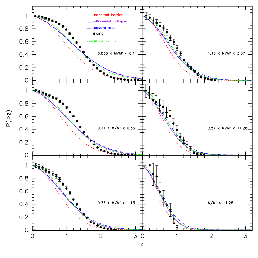
Figure 2: Cumulative distribution of dark halo formation times for halos identified at $z=0$. From top to bottom, panels show results for halos with masses in the range log${}_{10}M/h^{-1}M_{\odot}:$ 11.5-12, 12-12.5, 12.5-13, 13-13.5, and 13.5-14. Symbols show the measurements in GIF2; dotted curve shows the prediction associated the constant barrier spherical collapse model; dot-dashed curve shows the analytical fit equation (6) with $q=0.707$. Short-dashed and solid curves show the predictions associated with the square-root and ellipsoidal collapse based models.

3.1 The GIF2 simulation

The GIF2 simulation followed the evolution of $400^{3}$ particles in a periodic cube 110 $h^{-1}$Mpc on a side. The individual particle mass is $1.73\times 10^{9}\,h^{-1}M_{\odot}$, allowing us to study the formation histories of haloes which are one order of magnitude smaller in mass than was previously possible. Particle positions and velocities were stored at 50 output times, logarithmically spaced between $1+z=20$ and $1+z=1$. Halo and subhalo merger trees were constructed from these outputs as described by Tormen et al. (2004). Briefly, halos at a given redshift are identified as spherical objects which enclose the virial density appropriate the cosmological model at that redshift (computed using the spherical collapse model).

A merger history tree was constructed for each halo more massive than $10^{11.5}\,h^{-1}M_{\odot}$ (i.e., containing more than 180 particles) as follows. The progenitors of a halo of mass $M_{0}$ at $z_{0}$ are found by identifying in the previous output $z_{1}>z_{0}$ all haloes which contribute any number of particles to $M_{0}$. Of these, the progenitor which contributes the most mass to $M_{0}$ is called $M_{1}$. This procedure is then repeated, starting with $M_{1}$ at $z_{1}$, considering its progenitors in the previous output time $z_{2}>z_{1}$, and choosing from them the one, $M_{2}$, which contributes the most mass to $M_{1}$. In this way, the mass of the most massive progenitor is traced backwards in time, to high redshift.

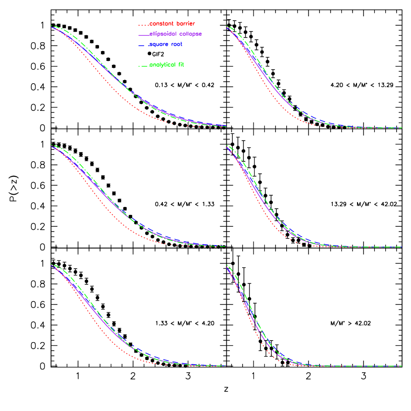
Figure 3: Same as previous figure, but now for halos identified at $z=0.5$. As before, the spherical model predicts lower formation redshifts than observed. Whereas the ellipsoidal collapse based expressions predict the median formation redshift reasonably well, they predict a broader range of redshifts than are observed.

We will present our results as a function of halo mass. We have estimated formation times for $5611$ halos with log${}_{10}(M/h^{-1}M_{\odot})$ in the range $11.5-12$, $2431$ in the range $12-12.5$, $892$ in the range $12.5-13$, $341$ in the range $13-13.5$, $92$ in the range $13.5-14$, and $29$ in the range $14-14.5$. These abundances are well fit by the formula of Sheth & Tormen (1999), so they are in better agreement with the ellipsoidal rather than spherical collapse model.

3.2 Cumulative distribution of formation times

Figure 2 shows the cumulative distribution of dark halo formation redshifts (i.e., equation 1) for halos identified at $z=0$. In general the analytical expressions obtained from the two different approximate solutions to the ellipsoidal collapse barrier problem—the (Sheth & Tormen, 2002) approximation for the first crossing distribution of the ellipsoidal collapse barrier, or the exact expression for the first crossing distribution of the square root barrier—are complicated. However, we have found that the predictions of the two ellipsoidal based models are quite well approximated by the expression for the spherical model with $n=0$, equation (6), by simply changing the value of $q$.

Different panels show results for the mass bins described above. The points show measurements in the GIF2 simulation, and the four curves show the formation time distributions associated with the $\mathrm{\Lambda}$CDM spherical collapse (dotted), ellipsoidal collapse (solid), square-root barrier approximation (dashed) and with equation (6) using $q=0.707$ (dot-dashed).

Again, the spherical collapse model severely underestimates the redshifts of halo formation. The two ellipsoidal collapse based estimates fare better, in the sense that they predict median formation redshifts which are closer to those seen in the simulation.

However, both ellipsoidal based estimates clearly predict a wider range of formation redshifts than is seen in the simulation—at fixed mass, the distribution of halo formation redshifts is narrower than predicted. This remains true for the formation time distribution of halos identified at $z=0.5$ shown in Figure 3.

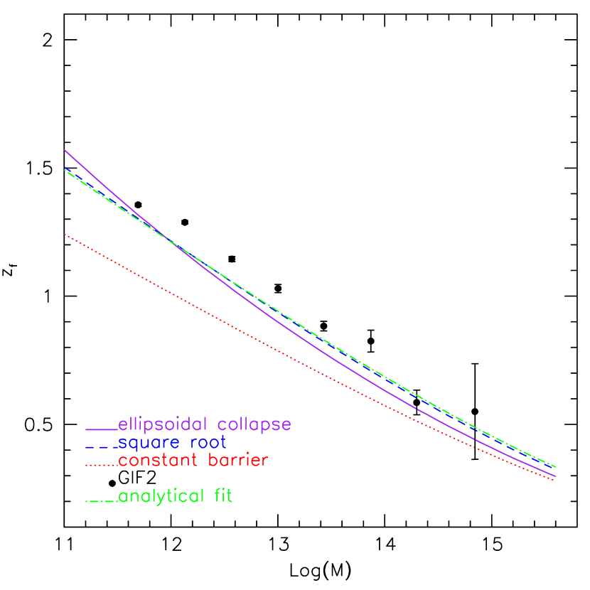
Figure 4: Median formation redshift for halos identified at $z=0$ as a function of halo mass. Points with (Poisson) error bars show our measurements in the GIF2 simulation. Smooth curves show the median formation times associated with three different models of halo formation: spherical collapse (dotted), ellipsoidal collapse (solid) and the square-root barrier approximation (short-dashed). Dot-dashed curve shows the prediction of equation (10) with $q=0.707$.

3.3 Mass-dependence of median formation time

Figure 4 shows the median formation redshift of halos identified at $z=0$ as a function of halo mass. Points show our measurements in the GIF2 simulation The simulation showes that massive halos formed more recently: the median formation redshift decreases with halo mass.

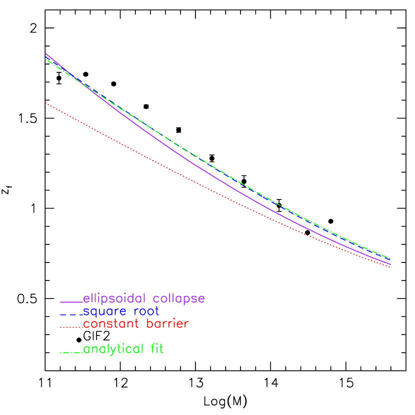
Figure 5: Same as previous Figure, but for halos identified at $z=0.5$ in the GIF2 simulation.

Smooth curves show the formation time distributions associated with three different models of halo formation: $\mathrm{\Lambda}$CDM spherical collapse (dotted), ellipsoidal collapse (solid) and the square-root approximation (short-dashed). In all cases, the model predictions for the median formation redshift were obtained by finding that $\bar{z}_{f}$ at which

$$\int_{M/2}^{M}{\rm d}m\,N(m,z_{\rm f}|M,z)={1\over 2}.$$ (9)

The Figure shows that halos less massive than $10^{14}h^{-1}M_{\odot}$ clearly form at higher redshifts than predicted by the spherical collapse model (dotted line). Both our estimates of the ellipsoidal collapse prediction are in substantially better agreement with the simulations. The prediction associated to equation (6) is given implicitely by inserting the median rescaled formation redshift $\bar{\omega}=0.974$ into equation (5), providing:

$$\delta_{\rm sc}(\bar{z}_{\rm f}|M,z_{0})=\delta_{\rm sc}(z_{0})+{0.974\over\sqrt{q}}\,\sqrt{S(M/2)-S(M)}.$$ (10)

The choice $q=0.707$ is shown by the dot-dashed line in the Figures; setting $q=0.6$ yields even better agreement with the simulations.

Fitting functions, accurate to a few percent, for $\delta_{\rm sc}(z)$ and $S(m)$ are available in the literature. For instance,

$$\delta_{\rm sc}(z)\approx D_{+}(z)\,\frac{3}{20}\,(12\pi)^{2/3}\,\Omega_{m}^{0.0055}\,$$ (11)

(Navarro et al., 1997), where $\Omega_{m}$ is the ratio of the background to the critical density at $z$, and

$$D_{+}(z)=\frac{5}{2}\,\Omega_{m}\Big{[}\Omega_{m}^{4/7}-\Omega_{\mathrm{\Lambda}}+\Big{(}1+\frac{1}{2}\Omega_{m}\Big{)}\Big{(}1+\frac{1}{70}\Omega_{\mathrm{\Lambda}}\Big{)}\Big{]}^{-1}$$ (12)

(Carroll et al., 1992), and, for a CDM power spectrum,

$$S(m)=A\left(1+2.208\bar{m}^{p}-0.7668\bar{m}^{2p}+0.7949\bar{m}^{3p}\right)^{-4/(9p)}$$ (13)

(Taruya & Suto, 2000), where $A$ is the normalization factor of the linear theory power spectrum at $z=0$ (so it depends on $\sigma_{8}$), $\bar{m}=m(h\Gamma)^{2}/10^{12}M_{\odot}$, where $\Gamma$ is the parameter which describes the shape of the power spectrum (typically $\Gamma\approx\Omega h$), and $p=0.0873$.

4 Discussion and Conclusions

Lacey & Cole (1993) defined the formation time of an object as the earliest time when at least half its mass was assembled into a single progenitor. We clarified the relation between this definition of formation time, and a quantity which arises in binary merger models of clustering (Appendix B). We have shown that insertion of spherical collapse based expressions in Lacey & Cole’s (1993) formalism for halo formation underestimates the redshifts of halo formation; this is consistent with previous work (Lin, Jing & Lin 2003). Ellipsoidal collapse based expressions are a marked improvement: although they result in formation redshift distributions which are broader than seen in simulations (Figures 2 and 3), they predict the median formation redshift quite well (Figure 4 and 5).

The fact that our predicted formation time distributions are broader than those seen in the simulation can be traced back to the fact that the low redshift progenitor mass functions from the excursion set approach are not in particularly good agreement with the simulations. This is similar to the findings of Sheth & Tormen (2002), who noted that some of the discrepancy was almost certainly due to the idealization that the steps in the excursion set walks are uncorrelated. Recent work has shown that there is some correlation between halo formation and environment (Sheth & Tormen, 2004; Gao et al., 2005; Harker et al., 2006; Wechsler et al., 2006)—this almost certainly indicates that a model with uncorrelated steps will be unable to provide a better description of the simulations. Nevertheless, the fact that the median formation redshifts are quite well reproduced by our model does represent progress.

Although the exact expressions associated with our models are complicated, we were able to find a useful fitting formula for the median formation redshift, equation (10), which we hope will be useful in studies which relate the formation times of halos to observable quantities.

Appendix A Explicit expressions for barrier crossing distributions

We are interested in walks which start from one barrier $B_{0}(S)$ and walk to another, $B_{1}(s)$, with $s>S$. Thus, the barrier to be crossed is of the form

$$B_{1}(s)-B_{0}(S)=\sqrt{q}\delta_{1}\Big{[}1+\beta\Big{(}\frac{s}{q\delta_{1}^{2}}\Big{)}^{\gamma}\Big{]}-\sqrt{q}\delta_{0}\Big{[}1+\beta\Big{(}\frac{S}{q\delta_{0}^{2}}\Big{)}^{\gamma}\,\Big{]}.$$ (14)

In the formulae $\delta_{0}$ and $\delta_{1}$ refer to the sferical collapse overdenisity at redshift $z_{0}$ and $z_{1}$. For barriers of this form, Sheth & Tormen (2002) showed that

$$f(s|S)ds \approx \frac{\mathrm{d}s}{s-S}\,\frac{|T(s|S)|}{\sqrt{2\pi(s-S)}}$$ (15)

$$\times\quad\exp{\Bigg{\{}-\frac{[B_{1}(s)-B_{0}(S)]^{2}}{2(s-S)}\Bigg{\}}},$$

where

$$T(s|S)=\sum^{5}_{n=0}\frac{(S-s)^{n}}{n!}\frac{\partial^{n}[B_{1}(s)-B_{0}(S)]}{\partial s^{n}}\,.$$ (16)

When $\beta=0$ and $q=1$, this reduces to the spherical collapse based expression used by Lacey & Cole (1993):

$$f(s|S)ds=\frac{\mathrm{d}s}{s-S}\,\frac{\delta_{1}-\delta_{0}}{\sqrt{2\pi(s-S)}}\,\exp\left\{-\frac{(\delta_{1}-\delta_{0})^{2}}{2(s-S)}\right\}.$$ (17)

When $\gamma=1/2$, then

$$B_{1}(s)-B_{0}(S)=\sqrt{q}(\delta_{1}-\delta_{0})-\beta\sqrt{S}+\beta\sqrt{s},$$ (18)

and the exact solution to this square-root barrier problem is

$$f(s|S)ds = \exp\left({w_{\beta}^{2}-\beta^{2}\over 4}\right)\times$$ (19)

$$\sum_{\lambda}\Bigg{(}\frac{S}{s}\Bigg{)}^{\frac{\lambda}{2}}\frac{D_{\lambda}(w_{\beta})\,D^{\prime}_{\lambda}(-\beta)}{I_{\lambda}(-\beta)}\frac{{\rm d}s}{2s}$$

(Breiman, 1966; Mahmood & Rajesh, 2005), where

$$w_{\beta}\equiv\frac{\sqrt{q}(\delta_{1}-\delta_{0})}{\sqrt{S}}-\beta,\quad I_{\lambda}(-\beta)\equiv\int^{\infty}_{-\beta}{\rm d}x\,D_{\lambda}^{2}(x),$$

and $D_{\lambda}(x)$ are parabolic cylinder functions which satisfy

$$D^{\prime}_{\lambda}(x)=(x/2)\,D_{\lambda}(x)-D_{\lambda+1}(x).$$

The sum is over the roots $\lambda$ defined by

$$D_{\lambda}(-\beta)=0,\quad{\rm so}\quad D^{\prime}_{\lambda}(-\beta)=-D_{\lambda+1}(-\beta).$$

Appendix B On the difference between halo formation and creation

The main text deals with halo formation as defined by Lacey & Cole (1993). Before continuing, it is worth mentioning that there is another context in which the term ‘halo formation’ arises—this is when the halo population is modeled as arising from a binary coagulation process of the type first described by Smoluchowski (1916). In this description, the time derivative of the halo mass function is thought of as the difference of two terms: one represents an increase in the number of halos of mass $m$ from the merger of two less massive objects, and the other is the decrease in the number of $m$-haloes which results as $m$-haloes themselves merge with other halos, creating more massive halos as a result:

$$\frac{{\rm d}n(m,t)}{{\rm d}t}=C(m,t)-D(m,t)$$ (20)

The gain term, the first on the right hand side above, is sometimes called the halo formation (Sheth & Pitman, 1997) or creation (Percival & Miller, 1999; Sheth, 2003) term. In what follows, we will use the word ‘creation’ to mean this term, and ‘formation’ to mean the quantity studied by Lacey & Cole.

Halo formation and creation are very different quantities, as we show below. Nevertheless, they are sometimes used interchangeably in the literature (e.g. Verde et al. (2001)). Here we show explicitly how to compute the Lacey-Cole formation time distribution from the Smoluchowski-type creation and destruction terms, with the primary aim of insuring that the error of confusing one for the other is not repeated.

In the Lacey-Cole picture, the formation time distribution of $M$-halos identified at $T$ is given by equation (2). In this case, one first integrates over the conditional mass function, and then takes a time derivative. Here, we will instead take the time derivative inside the integral over mass and compute it before integrating over mass, as suggested by equation (3). In this case, the integrand has the form of a time derivative which plays a central role in the Smoluchowski picture. In particular, we can write

$$\frac{{\rm d}N(m,t|M,T)}{{\rm d}t}=C(m,t|M,T)-D(m,t|M,T),$$ (21)

where $C$ and $D$ are now the creation and destruction terms associated with the progenitor mass function, evaluated explicitly in Sheth (2003).

This simple step shows explicitly that $p(t|M,T)$ can be written in terms of Smoluchowski-like quantities:

$$p(t|M,T)=\int_{M/2}^{M}{\rm d}m\,C(m,t|M,T)-\int_{M/2}^{M}{\rm d}m\,D(m,t|M,T).$$ (22)

A little thought shows why this works out so easily. Simply integrating the halo creation rate $C(m,t|M,T)$ over the range $M/2\leq m\leq M$ overestimates halo formation, since some of the halos created at $t$, with mass $3M/4\leq m\leq M$ say, may actually have been may created by binary mergers in which one of the halos had a mass in the range $M/2\leq m\leq 3M/4$. Such creations should not be counted towards halo formation, since formation refers to the earliest time that $m$ exceeds $M/2$. However, it is precisely this double-counting which the second term, the integral of $D(m,t|M,T)$ over the range $M/2\leq m\leq M$, removes. Note in particular that, whereas the formation time distribution $p(t|M,T)$ is related to Smoluchowski-type quantities, it is not the same as $C(m,t)$. For completeness, note that

$$C(m,t)=\int_{m}^{\infty}{\rm d}M\,n(M,T)\,C(m,t|M,T),$$ (23)

where $n(M,T)$ denotes the number density of halos of mass $M$ at time $T$.

References

- Bond et al. (1991) Bond, J. R., Cole, S., Efstathiou, G., & Kaiser, N. 1991, ApJ, 379, 440
- Breiman (1966) Breiman L., Proc. 5th Berk. Symp. Math. Statist. Prob. 2, 9
- Bullock et al. (2001) Bullock, J. S., Kravtsov, A. V., & Weinberg, D. H. 2001, Apj, 548, 33
- Carroll et al. (1992) Carroll, S. M., Press, W. H., & Turner, E. L. 1992, ARA&A, 30, 499
- Eke et al. (1996) Eke, V. R., Cole, S., & Frenk, C. S. 1996, MNRAS, 282, 263
- Gao et al. (2004) Gao, L., White, S. D. M., Jenkins, A., Stoehr, F., & Springel, V. 2004, MNRAS, 355, 819
- Gao et al. (2005) Gao, L., Springel, V., & White, S. D. M. 2005, MNRAS, 363, L66
- Gunn & Gott (1972) Gunn, J. E., & Gott, J. R. I. 1972, Apj, 176, 1
- Harker et al. (2006) Harker, G., Cole, S., Helly, J., Frenk, C., & Jenkins, A. 2006, MNRAS, 367, 1039
- Kauffmann et al. (1999) Kauffmann, G., Colberg, J. M., Diaferio, A., & White, S. D. M. 1999, MNRAS, 303, 188
- Lacey & Cole (1993) Lacey, C., & Cole, S. 1993, MNRAS, 262, 627
- Mahmood & Rajesh (2005) Mahmood, A., & Rajesh, R. 2005, ArXiv Astrophysics e-prints, arXiv:astro-ph/0502513
- McKay et al. (2005) McKay, T. A., et al. 2005, American Astronomical Society Meeting Abstracts, 206, #10.12
- Miller et al. (2005) Miller, C. J., et al. 2005, AJ, 130, 968
- Navarro et al. (1997) Navarro, J. F., Frenk, C. S., & White, S. D. M. 1997, ApJ, 490, 493
- Newman & Davis (2002) Newman, J. A., & Davis, M. 2002, ApJ, 564, 567
- Percival & Miller (1999) Percival, W., & Miller, L. 1999, MNRAS, 309, 823
- Press & Schechter (1974) Press, W. H., & Schechter, P. 1974, ApJ, 187, 425
- Seljak & Zaldarriaga (1996) Seljak, U., & Zaldarriaga, M. 1996, ApJ, 469, 437
- Sheth & Pitman (1997) Sheth, R. K., & Pitman, J. 1997, MNRAS, 289, 66 1057
- Sheth (1998) Sheth, R. K. 1998, MNRAS, 300,
- Sheth & Tormen (1999) Sheth, R. K., & Tormen, G. 1999, MNRAS, 308, 119
- Sheth, Mo & Tormen (2001) Sheth, R. K., Mo, H. J., & Tormen, G. 2001, MNRAS, 323, 1
- Sheth & Tormen (2002) Sheth, R. K., & Tormen, G. 2002, MNRAS, 329, 61
- Sheth et al. (2003) Sheth, R. K., et al. 2003, ApJ, 594, 225
- Sheth (2003) Sheth, R. K. 2003, MNRAS, 345, 1200
- Sheth & Tormen (2004) Sheth, R. K., & Tormen, G. 2004, MNRAS, 349, 1464
- Smoluchowski (1916) Smoluchowski, M. V. 1916, Zeitschrift fur Physik , 17, 557
- Taruya & Suto (2000) Taruya, A., & Suto, Y. 2000, ApJ, 542, 559
- Tormen (1998) Tormen, G. 1998, MNRAS, 297, 648
- Tormen et al. (2004) Tormen, G., Moscardini, L., & Yoshida, N. 2004, MNRAS, 350, 1397
- van den Bosch (2002) van den Bosch, F. C. 2002, MNRAS, 331, 98
- Verde et al. (2001) Verde, L., Kamionkowski, M., Mohr, J. J., & Benson, A. J. 2001, MNRAS, 321, L7
- Wechsler et al. (2002) Wechsler, R. H., Bullock, J. S., Primack, J. R., Kravtsov, A. V., & Dekel, A. 2002, ApJ, 568, 52
- Wechsler et al. (2006) Wechsler, R. H., Zentner, A. R., Bullock, J. S., & Kravtsov, A. V. 2005, ArXiv Astrophysics e-prints, arXiv:astro-ph/0512416