Swift and Chandra confirm the intensity-hardness correlation of the AXP 1RXS J170849.0–400910

Convincing evidence for long-term variations in the emission properties of the anomalous X-ray pulsar 1RXS J170849.0–400910 has been gathered in the last few years. In particular, and following the pulsar glitches of 1999 and 2001, XMM-Newton witnessed in 2003 a decline of the X-ray flux accompanied by a definite spectral softening. This suggested the existence of a correlation between the luminosity and the spectral hardness in this source, similar to that seen in the soft $\gamma$-repeater SGR 1806–20. Here we report on new Chandra and Swift observations of 1RXS J170849.0–400910 performed in 2004 and 2005, respectively. These observations confirm and strengthen the proposed correlation. The trend appears to have now reversed: the flux increased and the spectrum is now harder. The consequences of these observations for the twisted magnetosphere scenario for anomalous X-ray pulsars are briefly discussed.

1 Introduction

The Anomalous X–ray Pulsars (AXPs) are a small group of sources which stand apart from other known classes of X-ray pulsars. In particular, they all rotate with spin periods clustered in a very narrow range ($\mathrm{P}\sim 5-12$ s), they have large period derivatives ($\dot{\mathrm{P}}\sim 10^{-13}-10^{-10}$ s s^-1), and, except in one case (Camilo et al. 2006), deep searches for radio pulsations gave so far always negative results (Burgay et al. 2006). Another important characteristic which motivated the “anomalous” label (Mereghetti & Stella 1995; van Paradijs, Taam & van den Heuvel 1995), is their relatively high X-ray luminosity ($\sim 10^{34}-10^{36}\rm\ erg\;s^{-1}$), which cannot be accounted for by rotational energy losses alone, and no convincing evidence for a companion star was discovered so far for any of them. These considerations quite naturally led to the idea that a non-standard energy production mechanism is involved in their emission.

Many different models have been suggested all along for AXPs, such as they are accreting from a fossil disk, formed by the debris of the supernova event, or from a very low-mass companion (e.g. Mereghetti & Stella 1995; Mereghetti et al. 1998; Chatterjee et al. 2000; Perna et al. 2000; Alpar 2001). On the other hand, many observational properties support the idea of these sources being magnetars, i.e. isolated neutron stars powered by the decay of their huge magnetic fields ($\mathrm{B}\sim 10^{14}-10^{15}$ G; Duncan & Thompson 1992; Thompson & Duncan 1993, 1995, 1996). In fact, if the large observed spin-down is interpreted in terms of magneto-dipolar losses, all the AXPs seem to have magnetic fields in excess of the quantum critical field ($\mathrm{B}>4.4\times 10^{13}$ G). If this is the case, AXPs should be related to the Soft $\gamma-$ray Repeaters (SGRs), another class of X-ray sources thought to involve strongly magnetic neutron stars (see Woods & Thompson 2004 for a recent review on SGRs/AXPs). In recent years, intense monitoring programs revealed several common features between AXPs and SGRs, (i.e. short bursts, weak IR counterparts, high energy tails; Gavriil, Kaspi & Woods 2002; Kaspi et al. 2003; Israel et al. 2003; Kuiper, Hermsen & Méndez 2004), strengthening the idea of an underlying relation between these two classes of sources.

AXPs’ spectra in the X-ray range are well described by an empirical model, made by an absorbed black body ($\mathrm{kT}\sim 0.3-0.6$ keV) plus a relatively steep power law with (photon index $\Gamma\sim 2-4$), and a hard X-ray power-law tail with $\Gamma\sim 1$. Until a few years ago AXPs were commonly believed to be steady X-ray emitters (even if hints for variability were already found, see Iwasawa et al. 1992; Baykal & Swank 1996; Oosterbroek et al. 1998) but recently flux changes and spectral variability were detected, both long-term and with spin phase (Kaspi et al. 2003; Mereghetti et al. 2004; Rea et al. 2005).

1RXS J170849.0–400910 is a prototypical AXP, with a period of $\sim 11$ s (Sugizaki et al. 1997; Israel et al. 1999), a spin-down rate of $\sim 2\times 10^{-11}$s s^-1, and a soft spectrum (Israel et al. 2001). A phase-coherent timing solution, inferred thanks to the long Rossi-XTE monitoring of this source, led to the discovery of two glitches in the last few years, with very different post-glitch behavior (Kaspi, Lackey & Chakrabarty 2000; Dall’Osso et al. 2003; Kaspi & Gavriil 2003). In a very recent paper, Rea et al. (2005) showed that both the flux and spectral hardness reached a maximum level close to the two glitches that the source experienced in 1999 and 2001, and then decreased again in close correlation. Moreover, a long observation taken by BeppoSAX during the recovery from the second, more dramatic, glitch revealed evidence for a relatively broad absorption line at $\sim 8$ keV (Rea et al. 2003), not re-detected in more recent pointings (Rea et al. 2005). The spectral feature has been interpreted as a cyclotron resonance feature, yielding an estimate of the neutron star magnetic field of either $9.2\times 10^{11}$ G or $1.6\times 10^{15}$ G, in the case of electron or proton cyclotron absorption, respectively (Rea et al. 2003). In this paper we present new Swift (calibration) and Chandra observations of 1RXS J170849.0–400910. In Sect. 2 and 3 we describe the timing and spectral analysis of the Swift and Chandra observations, respectively, as well as reporting the results. Discussion follows in Sect. 4.

2 Swift observations

1RXS J170849.0–400910  was observed with the Swift satellite (Gehrels et al. 2004) a few times, being a calibrator for timing accuracy and for the wings of the Point Spread Function of the X–Ray Telescope (XRT, Burrows et al. 2005; see Table 1 for a detailed log of the observations). Here we focus on data taken in Window Timing (WT) mode and in Photon Counting (PC) mode longer than 1 ks. In particular, we used the PC data for spectral analysis and the PC + WT data for timing analysis. This choice is dictated by the fact that WT observations are affected by the source being at the edge of the window and during part of the observation the source fell outside the window, making difficult a secure evaluation of the instrument spectral response.

Table 1: Swift observations of 1RXS J170849.0–400910^a.

Obs. number	Mode	Exp. time (ks)	Start time
00050700001	LRPD	0.3	2005-01-29
	WT	10.3
	PC	0.7
00050700002	WT	0.2	2005-01-28
00050700006	WT	0.2	2005-03-23
	PC	2.3
00050700256	WT	0.6	2005-03-20
	PC	0.1
00050701001	LRPD	1.8	2005-01-30
	WT	16.5
	PC	2.3
00050701002	WT	0.7	2005-02-24
	PC	10.5
00050702001	PC	4.6	2005-02-02
00050702002	PC	1.7	2005-02-23
00050702003	PC	0.7	2005-03-23
00050702004	PC	0.5	2005-03-29

$a$ – Observations in bold face are the ones used for spectral and timing analysis. Observation in italic face have been used for timing analysis only. Observations shorter than 100 s were not listed above.

Data were analysed with the FTOOL task xrtpipeline (version build-14 under HEADAS 6.0). We applied standard screening criteria to the data (CCD temperature $T<-45^{\circ}$ C, eliminated hot pixels and bad aspect times). Hot and flickering pixels were removed. High background intervals due to dark current enhancements and bright Earth limb were removed too. Screened event files where then used to derive light curves and spectra. We included data between 0.5 and 10 keV, where PC response matrix is calibrated (we used the v.8 response matrices).

We extracted data from two WT observations. The extraction region is computed automatically by the analysis software and is a box 40 pixels along the WT strip, centered on source, encompassing $\sim 98\%$ of the Point Spread Function in this observing mode. We extracted photons from PC data from an annular region (3 pixels inner radius, 30 pixel outer radius) in order to avoid pile-up contamination. We consider standard grades 0–2 in WT and 0–12 in PC modes. Background spectra were taken from close-by regions free of sources.

2.1 Timing Analysis

Data were barycentered using the FTOOL task barycorr to correct the photon arrival times to the Solar system barycenter. A period search led to a clear detection of the neutron star spin period. The best period is $P=11.0027\pm 0.0003$ s (all errors in the text are given at $90\%$ confidence level). This has been derived with phase fitting techniques. This period is consistent with the extrapolation from known ephemerides at a constant period derivative (Kaspi & Gavriil 2003; Dall’Osso et al. 2003).

We divided the data in four energy bands then folded them at the neutron star spin period. The pulse profiles were then fitted with a sine wave obtaining the pulsed fraction (PF) in different energy ranges. We define here as PF the (semi-)amplitude of the best fitting sine to the normalised and background corrected folded data. We found a PF of $31\pm 2\%$, $39\pm 3\%$, $29\pm 4\%$ and $35\pm 7\%$ in the 0.2–10 keV, 0.2–2 keV, 2–4 keV and 4–10 keV energy bands, respectively.

Table 2: Spectral parameters of the Chandra ACIS–S observation (4.5 count s^-1) and of the simultaneous fits of the 5 longer Swift observations (0.3 count s^-1 on average). Fluxes are in the 0.5-10 keV band in units of $10^{-10}$ erg s^-1 cm^-2; column density were fixed at the XMM–Newton value of 1.36$\times 10^{22}$ cm^-2 (Rea et al. 2005; phabs model in XSPEC); all errors are at $90\%$ confidence level. Normalisations are in XSPEC units, i.e. the number of photons kev^-1 s^-1 cm^-2 at 1 keV.

	Chandra ACIS–S		Swift–XRT
	PL	PL+BB	PL	PL+BB
$\Gamma$	$3.11^{+0.02}_{-0.02}$	$2.74^{+0.02}_{-0.08}$	$2.93^{+0.04}_{-0.04}$	$2.70^{+0.16}_{-0.19}$
Norm PL	$0.064^{+0.002}_{-0.002}$	$0.033^{+0.004}_{-0.004}$	$0.056^{+0.02}_{-0.02}$	$0.031^{+0.008}_{-0.008}$
kT (keV)	–	$0.42^{+0.02}_{-0.02}$	–	$0.42^{+0.03}_{-0.02}$
Norm BB	–	$2.6^{+0.4}_{-0.6}\times 10^{-4}$	–	$4.7^{+1.2}_{-1.2}\times 10^{-4}$
Abs. Flux	$0.40^{+0.01}_{-0.03}$	$0.39^{+0.01}_{-0.02}$	$0.45^{+0.01}_{-0.01}$	$0.44^{+0.07}_{-0.06}$
Unabs. Flux	$1.31^{+0.06}_{-0.07}$	$1.30^{+0.07}_{-0.07}$	$1.74^{+0.07}_{-0.07}$	$1.43^{+0.04}_{-0.07}$
$\chi^{2}_{\rm red}$ (d.o.f.)	1.76 (154)	0.96 (152)	1.88 (125)	1.00 (123)

2.2 Spectral analysis

Spectral modelling was performed fitting together the five PC observations with exposure time longer than 1 ks, grouping the PC spectra to 60 counts per energy bin. The spectra were fitted in the 1–10 keV energy range since the high absorption made useless the data below 1 keV (Romano et al. 2005). For the PC data described above we generated the appropriate arf files with the FTOOL task xrtmkarf and used the latest v.8 response matrices. The spectral parameters are reported in Table 2.

We first fitted all the data with an absorbed (using phabs within XSPEC) power-law, leaving all the parameters free to vary. This model gave a reduced $\chi^{2}$ value of $\chi^{2}_{\rm red}=1.08$. The resulting column density is $N_{H}=(2.00^{+0.10}_{-0.16})\times 10^{22}\rm\ cm^{-2}$ and the power law photon index is $\Gamma=3.55^{+0.08}_{-0.17}$. We also consider a fit with the inclusion of a black body component. In this case we derive a lower column density $N_{H}=(1.37^{+0.27}_{-0.26})\times 10^{22}\rm\ cm^{-2}$ consistent with the value obtained by Rea et al. (2005). In addition we got $kT=0.42^{+0.04}_{-0.05}$ keV and $R=5.4\pm 1.5$ km (calculated at 5 kpc distance) as well as a flatter power law index $\Gamma=2.73^{+0.43}_{-0.52}$. Also in this case the fit is acceptable ($\chi^{2}_{\rm red}=1.01$). The inclusion of the black body component is significant at $3\,\sigma$ level (based on an F-test). The 0.5–10 keV absorbed (unabsorbed) flux is $4.4^{+0.07}_{-0.06}\times 10^{-11}\rm\ erg\;s^{-1}\rm\ cm^{-2}$ ($1.43^{+0.87}_{-0.45}\times 10^{-10}\rm\ erg\;s^{-1}\rm\ cm^{-2}$), with the power law component accounting for $72^{+7}_{-8}\%$ of the total flux. The power law component seems to be slightly decreased from the $82\pm 1\%$ for XMM-Newton. For comparison with previous spectra we computed also the same quantities fixing the column density to the XMM-Newton value ($N_{H,XMM}=(1.36\pm 0.04)\times 10^{22}\rm\ cm^{-2}$). Results are reported in Table 2 (in this case the power law contribution amounts to $71\pm 3\%$).

       

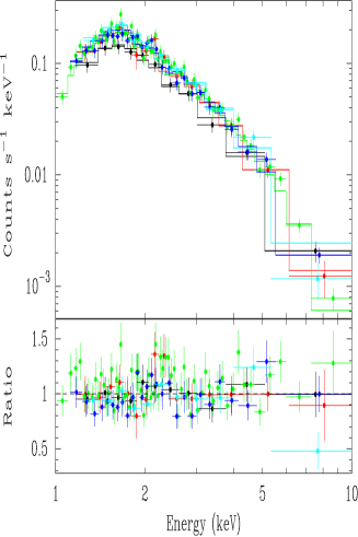
Figure 1: Left Panel: Spectra of the five longer Swift PC observations fitted with an absorbed blackbody plus a power-law. See Table 2 for further details on the spectral parameters. Right Panel: folded light curves in three energy bands, from top: 0.2–2 keV, 2–4 keV and 4–10 keV.

The 1RXS J170849.0–400910  spectrum and flux changed significantly from the XMM-Newton observation in August 2003. Constraining all the spectral parameters to the XMM-Newton values within their $90\%$ confidence intervals, the resulting fit is not acceptable with $\chi^{2}_{\rm red}=5.6$. In our best fit, the blackbody temperature remains consistent with the XMM-Newton value. The photon index instead decreased significantly and, at the same time, the flux increased. Interestingly, this is in good agreement with the correlation found in this source by Rea et al. (2005; see also below).

3 Chandra observation

1RXS J170849.0–400910  was observed by Chandra on 2004 July 3 (Obs-ID: 4605), for $\sim$30 ks with the Advanced CCD Imaging Spectrometer (ACIS). The ACIS CCDs S1, S2, S3, S4, I2 and I3 were on during the observation. In order to avoid the pile-up, the source was observed in the Continuous Clocking (CC) mode (CC33_FAINT; time resolution 2.85 ms). The source was positioned in the back-illuminated ACIS-S3 CCD on the nominal target position. The data were reprocessed using CIAO software (version 3.2). A detailed description on the analysis procedures, such as extraction regions, corrections and filtering applied to the source events and spectra can be found in Rea et al. (2005b).

In order to perform the timing analysis we corrected the events arrival times for the barycenter of the solar system (with the CIAO axbary tool) using the provided ephemeris. We used for the timing analysis only the events in the 0.3–8 keV energy range and the standard Xronos tools (version 5.19). One fundamental peak plus one harmonic were present in the power-spectrum. A period of $11.00223\pm 0.00005$ s has been detected referred to MJD 53189. The pulse profile has not changed with respect to the previous detection and the 0.3–8 keV PF is $35.4\pm 0.6\%$ (see Fig. 2 right panel).

Being the CC mode not yet spectrally calibrated, the TE mode response matrices (rmf) and ancillary files (arf) are generally used for the spectral analysis (see Rea et al. 2005b for a detailed description of the matrices extraction).

We fixed the absorption at $N_{H,XMM}=(1.36\pm 0.04)\times 10^{22}\rm\ cm^{-2}$ during the spectral fitting, because of the low statistics below 1 keV and especially because of well known calibration issues at 1–2 keV, as previously reported for other CC mode observations (Jonker et al 2003; Rea et al. 2005b). Actually, to avoid any CC mode calibration problem, all the fits were performed removing the data in the 0.9–2 keV range.

Also for this observation the best fitting model was the absorbed power law plus a blackbody. The blackbody temperature does not change much with respect to the XMM-Newton detection. The black body radius, $3.6\pm 0.4$ km, is however smaller and the decrease appears to be significant at or above the $3\sigma$ level. On the other hand the power law contribution in this Chandra observation was $80\pm 2\%$, still consistent with the XMM-Newton observation of the previous year. However, also in this case the photon index is moving harder and the flux increasing toward what Swift saw a year later (see Sec. 2). The spectral results are reported in Table 2 and Fig. 2 (left panel).

       

Figure 2: Left Panel: Chandra unfolded spectrum fitted with an absorbed blackbody plus a power-law. See Table 2 for further details on the spectral parameters. Right Panel: Chandra pulse profile in the 0.3–8.0 keV energy band.

4 Discussion

In this paper we present a new Chandra observation of the AXP 1RXS J170849.0–400910 and the first Swift observations of this source performed as a part of the XRT calibration programme.

We performed spectral and timing analysis of the data. The measured periods, even though affected by relatively large errors (see § 2.1), allows us to confirm that the sources is still in a phase of steady spin-down, following the last glitch.

Figure 3: Long term spectral history of 1RXS J170849.0–400910, correlated intensity-hardness variation (adapted from Rea et al. 2005). All reported fluxes are unabsorbed and in the 0.5–10 keV energy range. For clarity, the observations dates are: ROSAT – 1994; ASCA – 1996; first BeppoSAX – 1997; second BeppoSAX – 2001; Chandra-HETG – 2002; XMM-Newton – 2003; Chandra-CC – 2004; Swift – 2005.

The spectral analysis reveals the source undergoing significant spectral changes. Interestingly, the trend monitored following the glitches epochs (Kaspi, Lackey & Chakrabarty 2000; Dall’Osso et al. 2003; Kaspi & Gavriil 2003) and until the last XMM-Newton observation has now reversed (see Fig. 3). In particular, the source spectrum became much harder and the total unabsorbed flux in the 0.5-10 keV energy band a fraction $\sim 50\%$ higher with respect to that measured by XMM-Newton (Rea et al. 2005). Moreover, our analysis indicates that the flux increase is mainly due to an increase in the contribution of the thermal component, while the power law contribution to the total flux slightly decreased ($71\pm 3\%$, while the XMM-Newton measurement was $82\pm 1\%$).

In Rea et al. (2005) it has been proposed that the observed correlation between the X-ray flux and the spectral hardness may be explained within the “twisted magnetosphere” scenario (Thompson, Lyutikov & Kulkarni 2002; Beloborodov & Thompson 2006). The basic idea is that when a static twist is implanted, currents flow into the magnetosphere. As the twist angle $\Delta\phi_{\mathrm{NS}}$ grows, charge carriers (electrons and ions) provide an increasing optical depth to resonant cyclotron scattering and hence a flatter power-law. At the same time, the larger returning currents heat the star surface producing more thermal photons. Observations collected until 2003 were consistent with a scenario in which the twist angle was steadily increasing before the glitch epochs, culminating with glitches and a period of increased timing noise, and then decreasing, leading to a smaller flux and a softer spectrum. Both the Chandra and the Swift observations caught the source in a (relatively) hard, luminous state, revealing a reversed trend. However, the hardening-flux correlation is maintained, lending further support to this scenario.

What is particularly interesting, and measured here for the first time, is that since the last XMM-Newton observation the fraction of the total flux in the power-law component slightly decreased although the source spectrum became harder. This is somehow counter-intuitive. If taken at face value, it may be explained by the fact that, in the twisted magnetosphere model, both the spatial distributions of the magnetospheric currents (which act as “scattering medium”) and the surface emission induced by the returning currents (which acts as source of seed photons for the resonant scattering) are substantially anisotropic. Seed thermal photons and scatterers are confined in two different limited ranges of magnetic colatitudes, and both distributions move away from the poles for larger twist angle, although at a different rate. For instance, by using the expressions provided by Thompson, Lyutikov & Kulkarni (2002) for the differential luminosity induced by the returning currents, we can estimate that the center of the heated surface region moves from $\sim 37^{\circ}$ to $\sim 63^{\circ}$ in colatitude when $\Delta\phi_{\mathrm{NS}}$ increases from $\sim 0.1$ to 2 radians. Correspondingly, the peak of the efficiency of the scattering only shifts from $\sim 66^{\circ}$ to $\sim 72^{\circ}$ in colatitude. The size of the region interested by the scattering decreases to $\sim 37\%$, while the thermally emitting region becomes $\sim 5\%$ larger. Although the model is quite approximated, and the above numbers should be treated with care, this strong anisotropy suggests that the observed drop in the non-thermal flux may be due to the fact that a lower fraction of soft photons are intercepted by the cloud of scattering particles surrounding the star. Clearly, since the scattering depth increases with $\Delta\phi_{\mathrm{NS}}$, the power-law will be in any case flatter.

Our preliminary quantitative estimates show, however, that the increase in size of the thermally emitting region is not sufficient to account for the observed variation in the blackbody radius, at least on the basis of the original model by Thompson, Lyutikov & Kulkarni (2002). We only note in this respect that viewing geometry effects may be important, since the expected change in the position of the heated surface region may result in a larger portion of the emitting area coming into view.

Finally, we might speculate that the long-term variations shown in Fig. 3 may have a cyclic behavior with a recurrence time of $\approx 5$–10 yr. A possible explanation within the magnetar scenario might be the periodic twisting/untwisting of the star magnetosphere, where the characteristic dissipation time of a static twist is in fact $\approx 1$–10 yr according to the more recent estimates (Beloborodov & Thompson 2006). A detailed study of this intensity-hardness correlation, through further X-ray monitoring of this source, is needed in order to better constrain the model, and to infer information on the physical conditions in the star magnetosphere. Note that with a detailed modeling of this correlation we would be able in the near future to predict the occurrence of glitches and possibly also of bursts.

- (1) Alpar, M.A., 2001, ApJ, 554, 1245
- (2) Baykal, J., Swank, J., 1996, ApJ, 460, 470
- (3) Beloborodov, A.M., Thompson, C., 2006, ApJ submitted (astro-ph/0602417)
- (4) Burgay, M., et al. 2006, MNRAS, 372, 410
- (5) Burrows, D.N., et al., 2005, SSRv, 120, 165
- (6) Camilo, F., et al., 2006, Nature submitted
- (7) Chatterjee, P., Hernquist, L., Narayan, R., 2000, ApJ 534, 373
- (8) Dall’Osso, S., et al., 2003, ApJ, 499, 485
- (9) Duncan, R.C., Thompson, R., 1992, ApJ, 392, L9
- (10) Gavriil, F.P., Kaspi V.M., Woods, P.M., 2002, Nature, 419, 142
- (11) Gehrels, N., et al., 2004, ApJ, 611, 1005
- (12) Hill, J.E., et al., 2005, SPIE, 5898, 325
- (13) Israel, G.L., et al., 1999, ApJ, 518, L107
- (14) Israel, G.L., et al., 2001, ApJ, 560, L65
- (15) Israel, G.L., et al., 2003, ApJ, 589, L93
- (16) Iwasawa, K., et al., 1992, PASJ, 44, 9
- (17) Jonker, P., et al., 2003, MNRAS, 346, 684
- (18) Kaspi, V.M., Lackey, J.R., Chakrabarty, D., 2000, ApJ, 537, L31
- (19) Kaspi, V.M., Gavriil, F.P., 2003, ApJ, 596, L71
- (20) Kaspi, V.M., et al., 2003, ApJ, 588, L93
- (21) Kuiper, L., Hermsen, W., Mendez, M., 2004, ApJ, 613, 1173
- (22) Mereghetti, S., Stella, L., 1995, ApJ, 442, L17
- (23) Mereghetti, S., Israel, G.L., Stella, L., 1998, MNRAS, 296, 689
- (24) Mereghetti, S., et al., 2004, ApJ, 608, 427
- (25) Mereghetti, S., et al., 2005, ApJ, 628, 938
- (26) Oosterbroek, T., et al., 1998, A&A, 334, 925
- (27) Perna, R., Hernquist, L., Narayan, R., 2000, ApJ, 541, 344
- (28) Rea, N., et al., 2003, ApJ, 586, L65
- (29) Rea, N., et al., 2005, MNRAS 509
- (30) Rea, N., et al., 2005b, ApJ, 627, L133
- (31) Sugizaki, M., et al., 1997, PASJ, v.49, p.L25-L30
- (32) Thompson, C., Duncan, R.C., 1993, ApJ, 408, 194
- (33) Thompson, C., Duncan, R.C., 1995, MNRAS, 275, 255
- (34) Thompson, C., Duncan, R.C., 1996, ApJ, 473, 322
- (35) Thompson, C., Lyutikov, M., Kulkarni, S.R., 2002, ApJ, 574, 332
- (36) van Paradijs, J., Taam, R.E., van den Heuvel, E.P.J., 1995, A&A, 299, L41
- (37) Woods, P., Thompson, C., 2004, astro-ph/0406133