Tidal tails around globular clusters.
Are they a good tracer of cluster orbits?

Abstract

We present the results of detailed N-body simulations of clusters moving in a realistic Milky Way (MW) potential. The strong interaction with the bulge and the disk of the Galaxy leads to the formation of tidal tails, emanating from opposite sides of the cluster. Some characteristic features in the morphology and orientation of these streams are recognized and intepreted. The tails have a complex morphology, in particular when the cluster approaches its apogalacticon, showing multiple “arms” in remarkable similarity to the structures observed around NGC 288 and Willman 1.
Actually, the tails are generally good tracers of the cluster path quite far from the cluster center ($>7$–$8$ tidal radii), while on the smaller scale they are mainly pointing in the direction of the Galaxy center. In particular, the orientation of the inner part of the tails is highly correlated to the cluster orbital phase and to the local orbital angular acceleration. This implies that, in general, the orbital path cannot be estimated directly from the orientation of the tails, unless a sufficient large field around the cluster is available.

1 Introduction

It is commonly accepted that the present globular cluster (GC) population in the Milky Way represents the survivor of an initially more numerous one, depauperated by many disruptive processes (Murali & Weinberg, 1997a, b; Fall & Zhang, 2001).
The observational results obtained in the last decade have clearly confirmed the role played by the Milky Way environment on the GC evolution. Up to now, about $30$ galactic GCs show evidences of star depletion due to the tides caused by the field of the Galaxy.
The first evidence of the existence of tails surrounding GCs were achieved by Grillmair et al. (1995). Using colour-magnitude selected star counts in a dozen of galactic GCs, these authors showed that in the outer parts the stellar surface density profiles exceeded significantly the prediction of King models, extending also outside the tidal radius. They identified this surrounding material as made up of stars in the act of being tidally stripped from the cluster field and pointed out the importance of defining the large-scale distribution of extra-tidal stars on the sky to obtain constraints and traces for the GC orbits. More recently, other works confirmed and enlarged Grillmair et al.’s findings (Lehmann & Scholz, 1997; Testa et al., 2000; Leon et al., 2000; Siegel et al., 2001; Lee et al., 2003) giving evidence of the existence of many GCs surrounded by haloes or tails. For M92, Lee et al. (2003) found, also, that the extratidal material is not randomly distributed, being the density profile in the tails shallower for bright stars than for fainter ones.
This was the state of the art until the spectacular findings of two tidal tails emanating from the outer part of the Palomar 5 globular cluster and covering an arc of 10 degrees on the sky, corresponding to a (projected) length of 4 kpc at the distance of the cluster (Odenkirchen et al., 2001, 2002, 2003), obtained in the framework of the Sloan Digital Sky Survey (see also http://www.sdss.org). The stellar mass in the tails of this sparse, low-mass, halo cluster (with an estimated concentration parameter $c=0.7$) adds up to 1.2 times the mass of stars in the cluster, estimated in the range between $4.5\times 10^{3}M_{\odot}$ and $6\times 10^{3}M_{\odot}$. More recently, Grillmair & Dionatos (2006), still using SDSS data, have detected a continuation of Pal 5’s trailing tidal stream out to almost 19 degrees from the cluster. Combining this with the already known southern tail of Pal 5 yields a stream some $9$ kpc long on the sky.
Substantial tidal streams have recently been found associated with another low-mass and low-concentration GC in the SDSS area: NGC 5466. For this cluster Belokurov et al. (2006) reported giant tails extended for about 1 kpc in length and Grillmair & Johnson (2006), still using SDSS data, suggested that a $\approx 13$ kpc tidal stream of stars, extending from Bootes to Ursa Major, could also be associated with this system.
Together with the so-called Sagittarius stream (Mateo et al., 1998; Yanny et al., 2000; Martínez-Delgado et al., 2001; Majewski et al.,, 2003; Martínez-Delgado et al., 2004), which emerges from a dwarf galaxy that is currently being accreted by the Milky Way, Palomar 5 and NGC 5466 represent outstanding examples of ongoing tidal erosion of stellar systems in the Milky Way, being, up to now, also the only two globulars known for which such extended stream-like structures have been detected in the Galactic halo.

One of the first numerical investigations of the role played by a galactic tidal field on spherical stellar systems was that of Keenan & Innanen (1975), who studied the effect of realistic, time-varying tidal fields on the stellar orbits in a star cluster. They numerically integrated the equations of motion of three-bodies in models of spherically symmetric clusters which, in turn, move in eccentric orbits in the field of a model galaxy. One of the main conclusions of this work, which extended previous investigations made by King (1962), was that star clusters rotating in a retrograde sense are more stable in a tidal field than clusters with either direct rotation or no rotation due to the contribution of the Coriolis acceleration, acting in the same direction as the gravitational attraction for retrograde motion.
More recent works on weak tidal encounters based on a Fokker-Planck approach (Oh & Lin, 1992; Lee & Goodman, 1995) and self-consistent N-body techniques (Grillmair, 1998) confirmed that the interaction with external tidal field, combined with two-body relaxation in the core of the cluster and following replenishment of stars near the tidal radius, causes a flow of stars away from the cluster. The stripped stars remain in the vicinity of the cluster for several orbital periods, migrating either ahead of the cluster or falling behind, giving rise to a slow growth of the tidal tails.
A semi-analytic study of the development of tidal streams in galactic satellites was done by Johnston (1998), who gave estimates for the rate of growth of tidal tails. The effects of a realistic galactic tidal field (including both bulge, halo and disk) on GCs were investigated few years later by Combes et al. (1999). The main findings of the work were the following: stars escaped from the system go to populate two giant tidal tails along the cluster orbit; these tails present substructures, or clumps, attributed to strong shocks suffered by the cluster, and are preferentially formed by low mass stars.
Yim & Lee (2002) performed N-body simulations of GCs orbiting in a two-component galaxy model (with bulge and halo and no disk), using the direct-summation NBODY6 code (Aarseth, 1999) and focusing their attention, in particular, to the correlation between tidal tail elongation (described by mean of a ’position angle’, defined as the angle between the direction of the tail and the galactic center direction) and the cluster orbit. They found that, on circular orbits, tidal tails mantain an almost constant position angle ($\sim 60^{\circ}$), while GCs on non circular orbits show a variation of the position angle, according to orbital path and phase. The position angle increases when the cluster heads for perigalacticon. On the other hand, it tends to decreases when the cluster heads for apogalacticon.

Finally, some authors investigated also the dynamical evolution of some globular clusters in the tidal field of the Galaxy. In this context Dehnen et al. (2004) modelled the disruption of the globular cluster Pal 5 by galactic tides. Pal 5 is remarkable not only for its extended and massive tidal tails, but also for its very low mass and velocity dispersion. In order to understand these extreme properties, they performed many simulations aiming at reproducing the Pal 5 evolution along its orbit across the Milky Way. They explained the very large size of Pal 5 as the result of an expansion following the heating induced by the last strong disk shock about 150 Myr ago. The clumpy substructures detected in the tidal tails of Pal 5 are not reproduced in their simulations, so that they argued that these overdensities have been probably caused by interaction with Galactic substructures, such as giant molecular clouds, spiral arms, and dark matter clumps, which were not condsidered in their modeling. These simulations also predict the destruction of Pal 5 at its next disk crossing in about 110 Myr, suggesting that many more similar systems have once populated the inner parts of the Milky Way but have been transformed into debris streams by the Galactic tidal field.
In this context, it may be interesting mentioning the recent numerical work devoted to the study of smaller size systems (open clusters) in the MW tidal field (Chumak& Rastorguev, 2006), which confirms already known results in the case of the external part of GC tidal tails) about the alignement of stars of the tidal stream around a common orbit in the external field (Grillmair, 1998; Combes et al., 1999; Capuzzo Dolcetta et al., 2005).

In the above sketched theoretical and observational background, this work –which is inserted in a wider study on the dynamics of globular clusters in external tidal fields (Capuzzo Dolcetta et al., 2005; Di Matteo et al., 2005; Miocchi et al., 2006a, b)– is devoted to clarifying the connection among tidal tails and cluster orbit. We will describe and discuss the mechanisms that determines the tails morphology and how they depend on cluster trajectory and orbital phase.
For this purpose, we performed detailed $N-$body simulations (with $N=10^{5}$) of GCs moving in a realistic three-components (bulge, disk and halo) Milky Way potential.
The paper is organized as follows: in Sect.2 the Galaxy (Sect.2.1) and cluster (Sect.2.2) models adopted are presented, so as the numerical approach used; in Sect.3 we deal with the main results of our work, showing the formation and development of tidal tails around the cluster (Sect. 3.1), giving a qualitative approach for describing the tail morphology (Sect.3.2), presenting the numerical procedure adopted to fit tails direction (Sect.3.3) and, finally, discussing the tail-orbit alignement and its dependence on the orbital phase. In Sect.4, all the results are summarized and discussed.

2 Models and methods

2.1 Galaxy model

The model adopted for the Galactic mass distribution is that of Allen & Santillan (1991). It consists of a three component system: a spherical central bulge and a flattened disk, both of Miyamoto & Nagai (1975) form, plus a massive spherical halo. The gravitational potential is time indipendent, axysimmetric and given in an analytical form which is continuous together with its spatial derivatives.
Choosing a reference frame where the (x,y) plane coincides with the MW equatorial plane, the three components of the potential have, in cylindrical coordinates, the form:

$$\Phi_{B}(\omega,z) = -\frac{GM_{B}}{\sqrt{R^{2}+z^{2}+{b_{B}}^{2}}}$$ (1)

$$\Phi_{D}(\omega,z) = -\frac{GM_{D}}{\sqrt{R^{2}+\left(a_{D}+\sqrt{z^{2}+{b_{B}}^{2}}\right)^{2}}}$$ (2)

$$\Phi_{H}(r) = -\frac{GM(r)}{r}-\frac{GM_{H}}{1.02a_{H}}\left[-\frac{1.02}{1+(\frac{r}{a_{H}})^{1.02}}+ln\left(1+(\frac{r}{a_{H}})^{1.02}\right)\right]^{100}_{r},$$ (3)

where square brackets indicate the difference of the function evaluated at the 100 kpc and the generic $r=\sqrt{R^{2}+z^{2}}$ extremes. The parameters in the formulas above are listed in Table 1.

2.2 Cluster model and numerical method

The total initial mass of the cluster was chosen $M_{GC}=4.7\times 10^{5}$ M_⊙, i.e. a value compatible with masses of galactic globular clusters lying inside 4.5 kpc from the MW center (see Harris (1996) and Pryor & Meylan (1993)). The stellar mass spectrum of our cluster initial model was chosen as a Kroupa IMF sampled in the range $0.1M_{\odot}-20M_{\odot}$ and ”evolved” (in the sense of accounting for mass loss on the base of stellar evolution, according to Straniero et al. (1997); Dominguez et al. (1999)) up to $3$ Gyr (which corresponds to our assumed cluster age). In this interval of time all masses greater than $1.2$ M_⊙ go into the $0.5M_{\odot}-1.2M_{\odot}$ range. As in Capuzzo Dolcetta et al. (2005), we sampled this mass function into 12 mass classes, equally spaced in a linear scale, whose space and velocity distribution were evaluated by the adoption of a multimass King distribution (King, 1966; Da Costa & Freeman, 1976).
Obviously, the choice of $N=10^{5}$ as total number of cluster stars, together with the given value of $M_{GC}$ and of the above described mass function implied a rescaling of the star masses. Finally, to investigate the role played by the degree of cluster concentration, we considered clusters with two different values for the King concentration parameter $c$ (listed in Table 2).

The clusters move on the $y-z$ coordinate plane (the ($x,y$) plane corresponds to the Galactic disk), along orbits of different eccentricity, defined as

$$e=\frac{r_{a}-r_{p}}{r_{a}+r_{p}},$$ (5)

being $r_{p}$ and $r_{a}$, respectively, the GC pericentric and apocentric orbital distances. See Table 3 for GC orbital parameters and Fig.1 for a plot of the different simulated orbits.

All the simulations were performed by means of the TreeATD code, developed by two of us (Miocchi & Capuzzo-Dolcetta, 2002) which, as the original code by Barnes & Hut (1986), relies upon a tree-algorithm for the gravitational force evaluation on the large scale and on a direct summation on the small scale. The code was parallelized to run on high performance computers (via MPI routines) employing an original parallelization approach (see again (Miocchi & Capuzzo-Dolcetta, 2002, see)). The time-integration of the ‘particles’ trajectories is performed by a leap-frog algorithm that uses individual and variable time-steps according to the block-time scheme (Aarseth, 1985; Hernquist & Katz, 1989). See Miocchi et al. (2006a) for further details. The only constant of motion that can be significantly used to check the quality of the orbital time–integration is the total energy of the cluster, i.e. including the contribution of the external field to the GC potential energy. We saw that the upper bound of the relative error in the energy conservation, $\Delta E/E$, is $10^{-4}$ over the whole simulation time. This is no more than one order of magnitude worse than the error we got in a comparison simulation for the same GC in abscence of external field.

3 Results

3.1 Formation and evolution of tidal tails

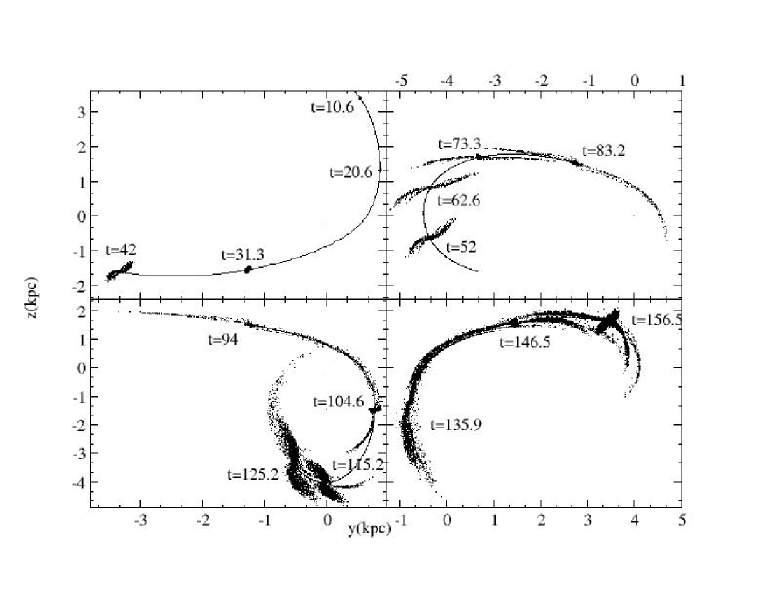
Figure 2: Some snapshots of the GC moving along the orbit I (see Table 3 for the orbital parameters). One time unit corresponds to about $1$ Myr.

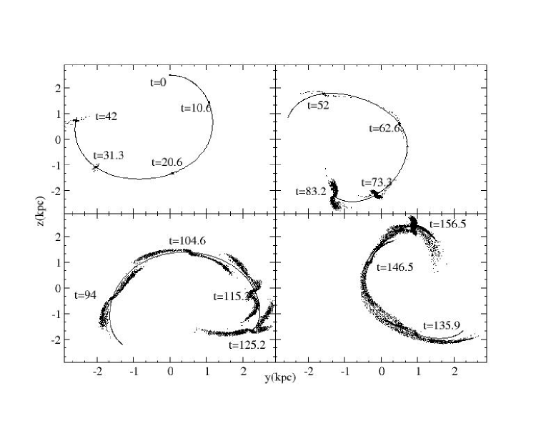
Figure 3: Some snapshots of the GC moving along the orbit II (see Table 3 for the orbital parameters). One time unit corresponds to about $1$ Myr.

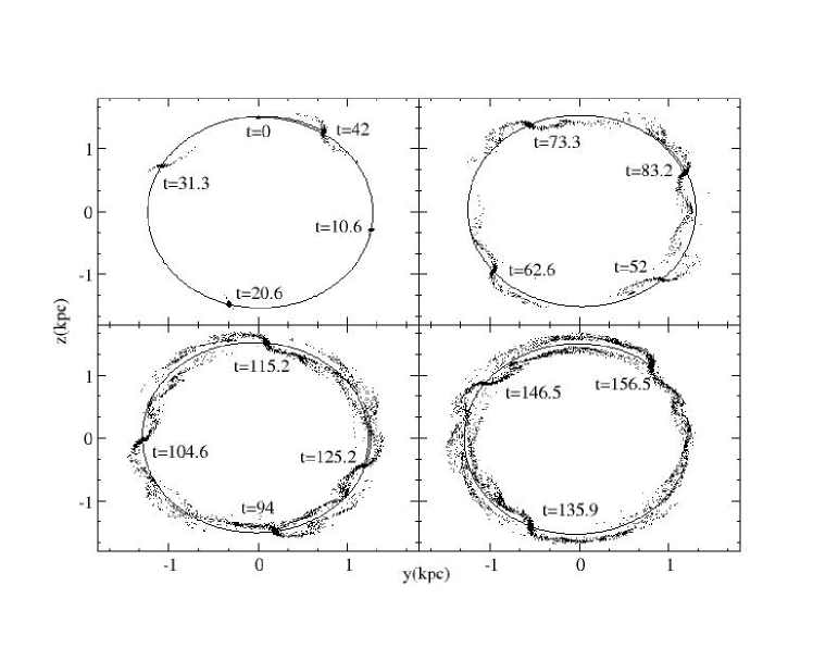
Figure 4: Some snapshots of the GC moving along the orbit III (see Table 3 for the orbital parameters). One time unit corresponds to about $1$ Myr.

In Figs. 2,3 and 4 the formation and subsequent evolution of tidal tails around the GC is shown, for all the simulations performed in the case of the least concentrated of the two GC models (the one with $c=0.81$ in Table 2). In the case of the more concentrated initial model cluster, the development of the tidal tails shows the same time dependence being just slightly less populated.
After about $5\times 10^{7}$ yr, tidal tails have clearly formed. They continuously accrete by the stars leaving the cluster, so that after $1.6\times 10^{8}$ yr, in the case of the quasi-circular orbit (orbit III), they are elongated for more than 1.5 kpc each. In general, the extention of the two cluster tails depends on the velocity of the cluster and its variation along the orbit. For the quasi-circular orbit (orbit III) this velocity is almost constant and the two tails have nearly the same length. For more eccentric orbits (orbit I and II), the tail extending between the GC and the pericenter is more elongated than the opposite tail, because the stars in the latter have smaller velocities than those belonging to the former one. In any case, the tail that precedes the cluster always extends slightly below the orbit, whereas the trailing one lies slightly above the orbit in agreement with what was observed for Pal 5. This feature can be explained considering the role played by the Coriolis acceleration, as we will see later.

As regards the tails orientation, these figures (Figs 2,3,4) clearly show the alignment of the outer part of the tails (at distances from the GC center $>7$–$8$ tidal radii) with the orbit. On the contrary, the alignment of the inner part is strongly correlated to both the orbit eccentricity and the GC location. Notice, indeed, that the inner tails are roughly aligned with the orbital path only when the cluster is near the perigalacticon of the more eccentric orbits (I and II, respectively shown in Fig.2 and Fig.3). This confirms previous results in Capuzzo Dolcetta et al. (2005), where analogous features were found for GCs movings in a triaxial potential.

It is also worth noting the peculiar morphology in the streams when the cluster is approaching the apocenter in the eccentric orbits (orbits I and II): tidal tails divide into “multiple arms”, two nearly elongated along the GC path, while the other two point to the galactic center (and anticenter) direction. At this regard, the tails observed around NGC288 (Leon et al., 2000) have a similar complex morphology, showing three different “arms”. Interestingly, this cluster has been estimated to be near its apogalacticon (Dinescu et al., 1999) in agreement with our results. Also the galactic satellite Willman 1 shows multi-directional stellar tails (Willman et al., 2006), which according to our results, could represent evidence that this system is approaching the apocenter on an eccentric orbit.

3.2 Tidal tails elongation: a qualitative description

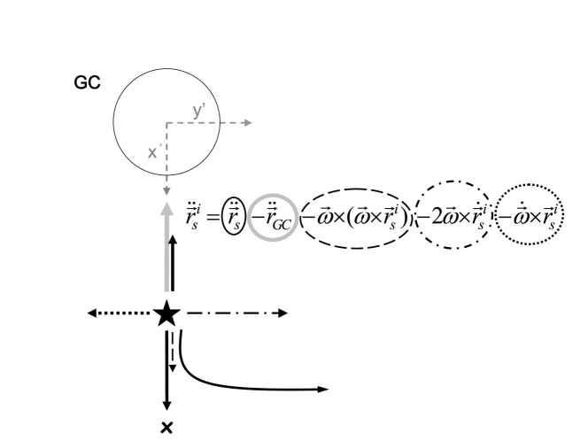
Figure 5: Interpretation of the S-shape of the inner tidal tail around a globular cluster. The different terms in the rhs of the displayed equation (Eq. 7) are represented in the plot as arrows of different line styles. Note that the last term in the equation is here plotted antiparallel to the Coriolis term as it occurs when the GC moves from pericenter to apocenter (see text). The Galactic potential (included in the first and second term) is assumed, for simplicity, spherical. The cross in the lower part of the figure represents the Galaxy center.

As anticipated in Di Matteo et al. (2005), the simplified scheme of the formation and shape of tidal tails around GCs can be understood by the motion of a star escaping from a cluster moving in a spherical potential. Let us consider a rotating reference frame with the origin in the cluster center-of-mass, the $(x^{\prime},y^{\prime})$ plane coinciding with the orbital plane and $x^{\prime}$ pointing to the galactic center. The equation of motion of the $i_{th}$ star belonging to the cluster that moves around the galaxy center with variable angular velocity $\omega$ is (see also Appendix A and Fig.5):

$$\ddot{\bf r}^{\prime}_{i}=\ddot{\bf r}_{i}-\ddot{\bf r}_{GC}-2\mbox{\boldmath{$\omega$}}\times\dot{\bf r}^{\prime}_{i}-\mbox{\boldmath{$\omega$}}\times\left(\mbox{\boldmath{$\omega$}}\times\bf{r}^{\prime}_{i}\right)-\dot{\mbox{\boldmath{$\omega$}}}\times\bf{r}^{\prime}_{i},$$ (6)

where ${\bf r}^{\prime}_{i}$ is the position vector in the rotating frame, while ${\bf r}_{i}$ and the position vector of the GC center-of-mass$,{\bf r}_{GC}$, refer to the inertial frame. For a star escaping through one of the unstable Lagrangian points along the $x^{\prime}$ axis, the first, second and fourth terms on the right-hand side of Eq. 6 are directed along the $x^{\prime}$ direction, while the third term (the Coriolis acceleration) and the fifth term are along $y^{\prime}$. The latter is parallel to the Coriolis term when $|\mbox{\boldmath{$\omega$}}|$ increases (i.e. moving from the apogalacticon to perigalacticon) and antiparallel when $|\mbox{\boldmath{$\omega$}}|$ decreases (moving from the perigalacticon to the apogalacticon). Consequently, these latter two terms ere responsible of the initial deviation of the tails from the radial direction and of the formation of the S-shape profile (see Capuzzo Dolcetta et al., 2005)).

3.3 The tail direction along the orbit

As a reliable quantitative definition of the tail orientation, we used the direction of the eigenvector corresponding to the greatest eigenvalue of the inertia tensor of a suitable portion of the cluster. More precisely, we considered the stars contained in an annulus centered at the cluster center-of-density (CD), as defined by Casertano & Hut (1985), and extending from $\approx 30$ pc up to a distance of $7$–$8$ tidal radii ($\sim 170$ pc). This region includes, indeed, the tail portion we call ”inner” part of the tails; this part is that usually detected in the observations. Note that in the study of Yim & Lee (2002) the direction of the tails was determined by eye, without any mathematically defined procedure.

For each configuration of the system:

• we evaluated the GC center-of-density;

• we selected all the stars distributed between $30$ pc and $170$ pc from the cluster CD (excluding stars lying inside $r<30$ pc, because this region corresponds to the spherical part of the system);

• we evaluated the inertia tensor and the corresponding eigenvalues and eigenvectors of the selected stars;

• we determined the eigenvector ${\bf u}$ corresponding to the maximum eigenvalue.

This eigenvector is parallel to the direction of the two tails having opposite orientation. In the following, we always refer to the tail internal to the cluster orbit.

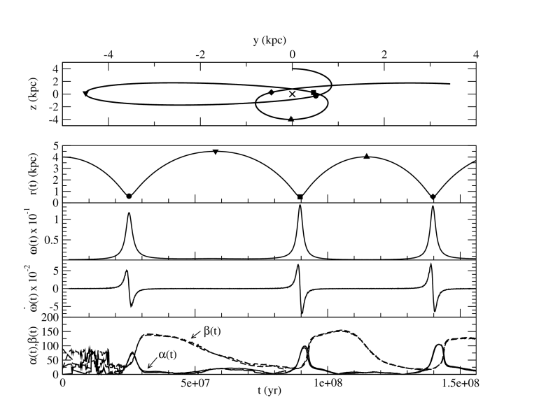
Figure 6: Tails direction for the GC moving on orbit I. From top to the bottom: Plot of the GC orbit (some points along the orbit are marked with different symbols) ; the cross indicates the Galaxy center. 2: distance in kpc of the GC from the Galaxy center, as a function of time. The different symbols correspond to that in the previous panel. 3: GC orbital angular velocity in rad/Myr, as a function of time. 4: angular acceleration in rad/$Myr^{2}$.5: solid curve: angle $\alpha$ formed by the inner part of the tails and the galactic center direction, vs time; dashed curve: angle $\beta$ formed by the inner part of the tails and the cluster velocity, vs time. Both angles are in degrees.

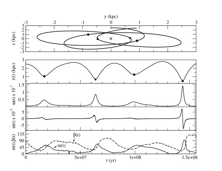
Figure 7: Same as Fig.6, but for the GC moving on orbit II.

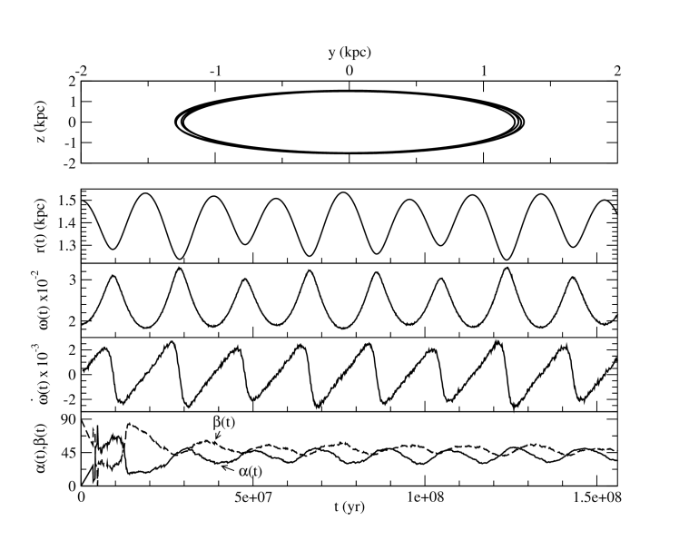
Figure 8: Same as Fig.6, but for the GC moving on orbit III.

The evolution of the tidal tail orientation is shown in Figs. 6, 7, 8.
These figures show the GC orbit and some kinematic quantities plotted as functions of time. From top to bottom we plot: the GC orbit (first panel), the distance $r$ of the cluster from the Galaxy center (second panel), the magnitude of the angular velocity vector $\omega$ (third panel), the time derivative of $|\mbox{\boldmath{$\omega$}}|$ (fourth panel). Finally, the fifth panel shows the evolution with time of two quantities: the angle

$$\alpha\equiv\cos^{-1}\left({\frac{{\bf u}\cdot{\bf r_{GC}}}{|{\bf u}||{\bf r_{GC}}|}}\right)$$ (7)

between the tail direction and that of the galactic center and the angle

$$\beta\equiv\cos^{-1}\left({\frac{{\bf u}\cdot\dot{\bf r}_{GC}}{|{\bf u}||\dot{\bf r}_{GC}|}}\right)$$ (8)

between the tail direction and the GC velocity vector (the angles assume values in the $[0^{\circ},180^{\circ}[$ interval).

3.3.1 Tail-Galaxy center alignement

In Figure 6, which refers to the orbit I, $\alpha$ is represented by two, barely distinguishable, solid curves, corresponding respectively to the GC with $c=1.02$ and $c=0.8$. The first result is that the time evolution of $\alpha$ is independent of the GC concentration (in the interval of $c$ studied); this means that the morphology and orientation of the tails depend on GC orbit, rather than on GC internal parameters.
Moreover, the tail is elongated toward the galactic center for most of the time: more in particular, if in Fig.6 we exclude the regions around the pericenter, the average value of $\alpha$ is $\sim 10^{\circ}$, i.e. the inner tail has only a slight deviation respect to the galactic center.

When approaching the pericenter, instead, the Coriolis and the $\dot{\mbox{\boldmath{$\omega$}}}$ terms (in Eq.6) are parallel and grow up. This induces a rapid alignement of the tails with the GC orbit. Beyond the pericenter, the Coriolis acceleration decreases and $\dot{\mbox{\boldmath{$\omega$}}}$ becomes antiparallel to the former. The net effect yields a realignment of the tails with the direction of the galactic center. Figure 7, which refers to orbit II, confirms the results found for the previous orbit.

Finally, Figure 8 shows the case of the quasi-circular orbit (orbit III). Along this orbit, both the distance of the GC from the galactic center and the orbital angular velocity are nearly constant. This leads to a roughly constant $\alpha\sim 40^{\circ}$. This suggests that the change in time of the orbital angular velocity is what determine the tails orientation.

3.3.2 Tail-orbit alignement

The dashed curve shown in the bottom panel of Figures 6,7 and 8 represents the angle $\beta$, previously defined. In the case of eccentric orbits, the first striking feature is that when approaching the pericenter the angle $\beta$ decreases, reaches a minimum at the pericenter and then increases moving away from the pericenter. The maximum value of $\beta$ is reached between the pericenter and the apocenter, depending on the shape of the GC orbit. However, in correspondence of the apocenter, $\beta$ is $\approx 90^{\circ}$ in agreement with the value $\alpha\approx 0^{\circ}$. At the apocenter the tail is aligned along the radial direction and roughly perpendicular to the GC velocity.

It is worth noting that, in all the cases considered here, the tidal tails deviate considerably by the GC velocity direction; only for very eccentric orbits and close to the pericenter, the angle $\beta$ reaches a minimum value of $\approx 17^{\circ}$. This indicates that the extrapolation of the cluster orbit from the elongation of this part of the tidal streams leads, in general, to predict GC paths with large errors.

4 Conclusions

This work is devoted to the study of the morphology and orientation of tidal tails surrounding globular clusters, in order to understand to what extent they trace the GC orbit and if some correlations exist between their orientation and the GC orbital phase.
The main findings of our work can be resumed as follows:

1. Tidal tails are good tracers of GC orbit only on the large scale, being the inner part of the streams never aligned with the GC path, unless the system moves on very eccentric orbit and close to the orbital pericenter.

2. A strong correlation exists between the orientation of the inner tails and GC orbital position: they tend to be more elongated along the GC orbit when the cluster approaches the pericenter, while, in turn, they tend to align toward the galactic center when the GC approaches the apocenter.

3. We have shown that a key role in determining the tails morphology is played by the orbital angular velocity of the system and its variation with time. In the case of the least eccentric orbit, a nearly constant angular velocity determines an almost constant orientation of tails with respect to the cluster orbit and the galactic center direction. The amplitude of $\dot{\mbox{\boldmath{$\omega$}}}$ contributes, too, to the alignement of tails with the GC path, in particular just beyond the pericenter.

4. The existing correlation between tails elongation and GC position along its orbit can be easily understood when referring to a non-inertial frame centered on the GC center, due to the role played by non inertial accelerations, as the Coriolis acceleration and that related to $\dot{\mbox{\boldmath{$\omega$}}}\times\bf{r}^{\prime}_{i}$.

We want to outline that our findings are in good agreement with some observational results. In particular we refer to the galactic globular clusters sample studied by Leon et al. (2000), considering the 7 clusters for which the reliability level of the observed tidal streams is highest and orbital parameters are available (Dinescu et al., 1999). Six clusters of this subsample (see Leon et al., 2000, Table 5) have tidal tails clearly elongated along the galactic center direction, and eccentricities greater than 0.62. This in agreement with our results that GCs, on eccentric orbits, have tidal tails elongated towards the galactic center for most of their path. The only exception is represented by NGC5139 ($\omega$ Cen), which has tidal tails deviating from the galactocentric direction and extending towards the galactic plane; this situation does not contradict our results considering that NGC5139 is presently only 1.3 kpc above the galactic disk and is most probably undergoing a strong disk-shocking.

The simulations also reproduce the formation of multiple tails around globular clusters, as observed for NGC288 (Leon et al., 2000) and for the galactic satellite Willman 1 (Willman et al., 2006). Our simulations show that these features are expected for GCs on eccentric orbits near their apogalacticon, while they are absent in the case of GCs moving on less eccentric orbits. Actually, their formation can be explained by the behaviour of the Coriolis acceleration along the orbit: when its value is large, stars escaping from the cluster are pushed toward the orbital path. This is particularly evident around the pericenter; at the apocenter, where the Coriolis acceleration is weaker, stars tend to escape from the cluster more radially. At every pericenter passage, this effect produce a new tidal tail roughly aligned to the cluster path.

5 Acknowledgements

The authors acknowledge the Centro de Astrobiologiá (Madrid, Spain) for the use of its computational facilities. We also thank prof. D. Heggie for useful comments and for pointing us an error in one of the figure catpions.

Appendix A Equations of motion in the non-inertial reference frame

Using a no-inertial reference frame $(x^{\prime},y^{\prime},z^{\prime})$ with the origin in the cluster center-of-mass, with the $(x^{\prime},y^{\prime})$ plane coinciding with the cluster orbital plane and $x^{\prime}$ always pointing to the galactic center (so that this reference frame rotates with the GC angular velocity $\omega$ respect to the inertial reference system $(x,y,z)$), the position of the $i-th$ star in the galactocentric $(x,y,z)$ reference frame can be expressed simply as:

$${\bf r}_{i}={\bf r}_{GC}+{\bf r^{\prime}}_{i}$$ (A1)

being ${\bf r}_{GC}$ the position of the cluster center-of-mass in the inertial system. Rewriting the previous equation in terms of the $(x^{\prime},y^{\prime})$ components (we omit the $z^{\prime}$ one for simplicity) we have:

$$x_{i}\mbox{\boldmath{$\hat{x}$}}+y_{i}\mbox{\boldmath{$\hat{y}$}}=x_{GC}\mbox{\boldmath{$\hat{x}$}}+y_{GC}\mbox{\boldmath{$\hat{y}$}}+x^{\prime}_{i}\mbox{\boldmath{$\hat{x^{\prime}}$}}+y^{\prime}_{i}\mbox{\boldmath{$\hat{y^{\prime}}$}}$$ (A2)

being $\hat{x}$,$\hat{y}$ and $\hat{x^{\prime}}$,$\hat{y^{\prime}}$ the unity vectors in the two frames, respectively. Derivating Eq.A2 with respect to time $t$, one obtains:

$$\dot{x}_{i}\mbox{\boldmath{$\hat{x}$}}+\dot{y}_{i}\mbox{\boldmath{$\hat{y}$}} = \dot{x}_{GC}\mbox{\boldmath{$\hat{x}$}}+\dot{y}_{GC}\mbox{\boldmath{$\hat{y}$}}+\dot{x^{\prime}}_{i}\mbox{\boldmath{$\hat{x^{\prime}}$}}+\dot{y^{\prime}}_{i}\mbox{\boldmath{$\hat{y^{\prime}}$}}+x^{\prime}_{i}\mbox{\boldmath{$\dot{\hat{x}^{\prime}}$}}+y^{\prime}_{i}\mbox{\boldmath{$\dot{\hat{y}^{\prime}}$}}=$$ (A4)

$$\dot{x}_{GC}\mbox{\boldmath{$\hat{x}$}}+\dot{y}_{GC}\mbox{\boldmath{$\hat{y}$}}+\dot{x^{\prime}}_{i}\mbox{\boldmath{$\hat{x^{\prime}}$}}+\dot{y^{\prime}}_{i}\mbox{\boldmath{$\hat{y^{\prime}}$}}+\mbox{\boldmath{$\omega$}}\times(x^{\prime}_{i}\mbox{\boldmath{$\hat{x^{\prime}}$}}+y^{\prime}_{i}\mbox{\boldmath{$\hat{y^{\prime}}$}})$$

being

$$\dot{\hat{x}^{\prime}} = \mbox{\boldmath{$\omega$}}\times\mbox{\boldmath{$\hat{x^{\prime}}$}}$$ (A5)

$$\dot{\hat{y}^{\prime}} = \mbox{\boldmath{$\omega$}}\times\mbox{\boldmath{$\hat{y^{\prime}}$}}$$ (A6)

Derivating Eq.A4 with respect to time $t$ and using Eqs. A5-A6, one obtains:

$$\ddot{x}_{i}\mbox{\boldmath{$\hat{x}$}}+\ddot{y}_{i}\mbox{\boldmath{$\hat{y}$}} = \ddot{x}_{GC}\mbox{\boldmath{$\hat{x}$}}+\ddot{y}_{GC}\mbox{\boldmath{$\hat{y}$}}+\ddot{x^{\prime}}_{i}\mbox{\boldmath{$\hat{x^{\prime}}$}}+\ddot{y^{\prime}}_{i}\mbox{\boldmath{$\hat{y^{\prime}}$}}+2\mbox{\boldmath{$\omega$}}\times(\dot{x^{\prime}}_{i}\mbox{\boldmath{$\hat{x^{\prime}}$}}+\dot{y^{\prime}}_{i}\mbox{\boldmath{$\hat{y^{\prime}}$}})+$$ (A8)

$$\mbox{\boldmath{$\omega$}}\times\left(\mbox{\boldmath{$\omega$}}\times(x^{\prime}_{i}\mbox{\boldmath{$\hat{x^{\prime}}$}}+y^{\prime}_{i}\mbox{\boldmath{$\hat{y^{\prime}}$}})\right)+\dot{\mbox{\boldmath{$\omega$}}}\times(x^{\prime}_{i}\mbox{\boldmath{$\hat{x^{\prime}}$}}+y^{\prime}_{i}\mbox{\boldmath{$\hat{y^{\prime}}$}})$$

and so, finally, Eq.6.

Figure 1: Orbits of a point mass with the initial position and velocity given in Table 3 in the MW potential (see sect. 2.1). Top panel: orbit I; central panel: orbit II; bottom panel: orbit III.

Table 1: Parameters for the Galactic model (Allen & Santillan, 1991)

Bulge	$M_{B}$	$1.41\times 10^{10}M_{\odot}$
	$b_{B}$	387.3 pc
Disk	$M_{D}$	$8.56\times 10^{10}M_{\odot}$
	$a_{D}$	5317.8 pc
	$b_{D}$	250.00 pc
Halo	$M_{H}$	$10.7\times 10^{10}M_{\odot}$
	$a_{H}$	12000 pc

Table 2: GC structural parameters

$M_{GC}[M_{\odot}]$	$r_{c}$ [pc]	$r_{t}$ [pc]	$c=log(r_{t}/r_{c})$	$\sigma$[km/s]
$4.7\times 10^{5}$	2.2	23.5	1.03	10.5
$4.7\times 10^{5}$	3.5	22.1	0.81	10.5

Note. — Col. (1): cluster total mass. Col. (2-4): core radius, cutoff radius and concentration parameter of the King’s model. Col. (5): central velocity dispersion.

Table 3: GC initial orbital parameters .

Orbit ID	$x$[pc]	$y$[pc]	$z$[pc]	$v_{x}$[km/s]	$v_{y}$[km/s]	$v_{z}$[km/s]	$e$
I	0.	0.	4000.	0.	53.3	0.	0.8
II	0.	0.	2500.	0.	116.7	0.	0.7
III	0.	0.	1500.	0.	200.0	0.	0.1

Note. — Col. (1): orbit identification. Col. (2-7): cluster initial center-of-mass position and velocity components. Col (8): orbit eccentricity [Eq.(5)]

References

- Allen & Santillan (1991) Allen, C., Santillan, A. 1991, RevMexAA, 22, 255
- Aarseth (1985) Aarseth, S.J. 1985, in ‘Multiple time scales’, Acad. Press, 378
- Aarseth (1999) Aarseth, S. J. 1999, PASP, 111, 1333
- Barnes & Hut (1986) Barnes, J. & Hut, P. 1986, Nature, 324, 446
- Baumgardt & Makino (2003) Baumgardt, H., Makino, J. 2003, MNRAS, 340, 227
- Belokurov et al. (2006) Belokurov, V., Evans, N. W., Irwin, M. J., Hewett, P. C., Wilkinson, M. I. 2006, ApJL,637,29
- Capuzzo Dolcetta et al. (2005) Capuzzo Dolcetta, R., Di Matteo, P. & Miocchi, P. 2005, AJ, 129, 1906
- Casertano & Hut (1985) Casertano, S., Hut, P. 1985, ApJ, 298, 80
- Chumak& Rastorguev (2006) Chumak, Ya. O., Rastorguev, A. S. 2006, Astronomy Letters, 32, 446
- Combes et al. (1999) Combes, F., Leon, S, Meylan, G. 1999, A&A, 352, 149
- Da Costa & Freeman (1976) Da Costa, G. S., Freeman, K. C. 1976, ApJ, 206, 128
- Dehnen et al. (2004) Dehnen, W., Odenkirchen, M., Grebel, E. K., Rix, H. W. 2004, AJ, 127, 2753
- Di Matteo et al. (2005) Di Matteo, P., Capuzzo Dolcetta, R., Miocchi, P., 2005, Celest. Mech., 91, 59
- Dinescu et al. (1999) Dinescu, D.I., Girard, T.M. & van Altena, W.F. 1999, AJ, 117, 1792
- Dominguez et al. (1999) Dominguez, I., Chieffi, A., Limongi, M. & Straniero, O. 1997, ApJ, 524-1, 226
- Fall & Zhang (2001) Fall, S. M., Zhang, Q. 2001, ApJ, 561, 751
- Grillmair et al. (1995) Grillmair, C. J., Freeman, K. C., Irwin, M., Quinn, P. J. 1995, AJ, 109, 2553
- Grillmair (1998) Grillmair, C. J. 1998, in D. Zaritsky ed., ASP Conf. Ser. vol.136, Galactic Halos: A UC Santa Cruz Workshop, Astron. Soc. Pac., San Francisco, p.45
- Grillmair & Dionatos (2006) Grillmair, C. J., Dionatos, O. 2006, ApJ, 641, L37
- Grillmair & Johnson (2006) Grillmair, C. J., Johnson, R. 2006, ApJ, 639, L17
- Harris (1996) Harris, W.E. 1996, AJ, 112, 1487
- Hernquist & Katz (1989) Hernquist, L. & Katz, N. 1989, ApJS, 70, 419
- Johnston (1998) Johnston, K. V. 1998, ApJ, 495, 297
- Keenan & Innanen (1975) Keenan, D. W., Innanen, K. A. 1975, AJ, 80, 290
- King (1962) King, I. R. 1962, AJ, 67, 471
- King (1966) King, I. R. 1966, AJ, 71, 276
- Kroupa (2001) Kroupa, P., 2001, MNRAS, 322, 231
- Lee & Goodman (1995) Lee, H. M., Goodman, J. 1995, ApJ, 443, 109
- Lehmann & Scholz (1997) Lehmann, I., Scholz, R.D. 1997, A&A, 320, 776
- Lee et al. (2003) Lee, K. H., Lee, H. M., Fahlman, G. G., Lee, M. G. 2003, AJ, 126, 815
- Leon et al. (2000) Leon, S., Meylan, G., Combes, F. 2000, A&A, 359, 907
- Majewski et al., (2003) Majewski, S. R., Skrutskie, M. F., Weinberg, M. D., Ostheimer, J. C. 2003, ApJ, 599, 1082
- Martínez-Delgado et al. (2001) Martínez-Delgado, D., Aparicio, A., Gómez-Flechoso, M. A., Carrera, R. 2001, ApJ, 549, L199
- Martínez-Delgado et al. (2004) Martínez-Delgado, D., Gómez-Flechoso, M. A., Aparicio, A., Carrera, R. 2004, ApJ, 601, 242
- Mateo et al. (1998) Mateo, M., Olszewski, E. W., Morrison, H. L. 1998, ApJ, 508, L55
- Miocchi & Capuzzo-Dolcetta (2002) Miocchi, P. & Capuzzo-Dolcetta, R. 2002, A&A, 382, 758
- Miocchi et al. (2006a) Miocchi, P., Capuzzo-Dolcetta, R., Di Matteo, P., & Vicari, A. 2006, ApJ, 644, 940
- Miocchi et al. (2006b) Miocchi, P., Capuzzo-Dolcetta, R., Di Matteo, P., contribution to ”Globular Clusters: Guides to Galaxies”, March 6th-10th, 2006, astro-ph/0605008
- Murali & Weinberg (1997a) Murali, C., Weinberg, M. D. 1997a, MNRAS, 291, 717
- Murali & Weinberg (1997b) Murali, C., Weinberg, M. D. 1997b, MNRAS, 288, 749
- Miyamoto & Nagai (1975) Miyamoto, M. & Nagai, R. 1975, Pub.Astr.Soc.Japan, 27, 533
- Odenkirchen et al. (2001) Odenkirchen, M., Grebel, E. K., Rockosi, C. M., Dehnen, W., Ibata, R., Rix, H. W., Stolte, A., Wolf, C., Anderson, J. E. Jr., Bahcall, N. A., Brinkmann, J., Csabai, I., Hennessy, G., Hindsley, R. B., Ivezic, Z., Lupton, R. H., Munn, J. A., Pier, J. R., Stoughton, C., York, D. G. 2001, ApJ, 548, L165
- Odenkirchen et al. (2002) Odenkirchen, M., Grebel, E. K., Dehnen, W., Rix, H. W., Cudworth, K. M. 2002, AJ, 124, 1497
- Odenkirchen et al. (2003) Odenkirchen, M., Grebel, E, K., Dehnen, W, Rix, H. W., Yanny, B., Newberg, H. J., Rockosi, C. M., Martínez-Delgado, D., Brinkmann, J., Pier, J. R. 2003, AJ, 126, 2385
- Oh & Lin (1992) Oh, K. S., Lin, D. N. C. 1992, ApJ, 386, 51
- Pryor & Meylan (1993) Pryor, T., Meylan, G. 1993, in Structure and Dynamics of Globular Clusters, ed. S. G. Djorgovski, & G. Meylan (San Fransisco), ASP Conf. Ser., 50, 357
- Siegel et al. (2001) Siegel, M. H., Majewski, S. R., Cudworth, K. M., Takamiya, M. 2001, AJ, 121, 935
- Straniero et al. (1997) Straniero, O., Chieffi, A. & Limongi, M. 1997, ApJ, 490, 425.
- Testa et al. (2000) Testa, V., Zaggia, S. R., Andreon, S., Longo, G., Scaramella, R., Djorgovski, S. G., de Carvalho, R. 2000, A&A, 356, 127
- Yanny et al. (2000) Yanny, B., Newberg, H.J., Kent, S., Laurent-Muehleisen, S. A., Pier, J. R., Richards, G. T., Stoughton, C., Anderson, J. E., Jr., Annis, J., Brinkmann, J., Chen, B., Csabai, I., Doi, M., Fukugita, M., Hennessy, G. S.; Ivezić, ., Knapp, G. R., Lupton, R., Munn, J. A., Nash, T., Rockosi, C. M., Schneider, D. P., Smith, J. A., York, D. G.2000, ApJ, 540, 825
- Yim & Lee (2002) Yim, K., Lee, H. M. 2002, JKAS, 35, 75
- Willman et al. (2006) Willman, B., Masjedi, M., Hogg, D. W., Dalcanton, J. J., Martinez-Delgado, D., Blanton, M., West, A. A., Dotter, A., Chaboyer, B. 2006, astro-ph/0603486