Electron-ion coupling upstream of relativistic collisionless shocks

Abstract

It is argued and demonstrated by particle-in-cell simulations that the synchrotron maser instability could develop at the front of a relativistic, magnetized shock. The instability generates strong low-frequency electromagnetic waves propagating both upstream and downstream of the shock. Upstream of the shock, these waves make electrons lag behind ions so that a longitudinal electric field arises and the electrons are accelerated up to the ion kinetic energy. Then thermalization at the shock front results in a plasma with equal temperatures of electrons and ions. Downstream of the shock, the amplitude of the maser-generated wave may exceed the strength of the shock-compressed background magnetic field. In this case the shock-accelerated particles radiate via nonlinear Compton scattering rather than via a synchrotron mechanism. The spectrum of the radiation differs, in the low-frequency band, from that of the synchrotron radiation, providing possible observational tests of the model.

1 Introduction.

Relativistic shocks are supposed to play an important role in various astrophysical objects, e.g., in pulsar wind nebulae, active galactic nuclei, gamma-ray bursts. In all these cases shocks are collisionless therefore some plasma instabilities are assumed to provide dissipation necessary for the final thermalization of the flow. An important point is that in relativistic case, plasma instabilities are generally electromagnetic and therefore strong low-frequency electromagnetic waves could be emitted. If a non-negligible magnetic field is presented in the upstream flow, the synchrotron maser instability develops at the shock front (Langdon, Arons & Max 1988).

One-dimensional particle-in-cell (PIC) simulations of relativistic magnetized shocks in electron-positron and electron-positron-ion plasmas (Gallant et al. 1992; Hoshino et al. 1992) demonstrate intensive electromagnetic waves both upstream (precursor) and downstream of the shock; these waves are generated by synchrotron maser instability at the shock front. It was shown that the precursor takes a few-per cent of the flow energy. One can anticipate that the upstream flow could be significantly affected by interaction with the precursor; this in turn could significantly influence the structure of the shock. For example, absorption of the precursor would result in strong deceleration and heating of the flow even though the energy of the precursor is small compared with the total energy of the flow; this follows immediately from the conservation of energy and momentum in the ultrarelativistic case. Of course true absorption is negligibly weak in the case of interest; the precursor radiation should be eventually absorbed via non-linear plasma processes, e.g., induced scattering. In this case one can anticipate formation of non-thermal particle distribution already in the upstream flow, which could significantly affect particle acceleration process at the shock.

Investigation of complicated nonlinear absorption of the precursor wave is beyond the scope of the present research; this would require multidimensional simulations at a very large scale. The aim of the present study is to consider a simpler mechanism of interaction between the electromagnetic precursor and the upstream flow. This mechanism does not assume absorption; however, it operates only in electron-ion flows. The basic idea is the following. Because electrons interact with the waves whereas ions do not, some velocity difference arises between the electron and ion flows illuminated by powerful electromagnetic waves. This is not associated with absorption; just because electrons experience relativistic oscillations in the field of the strong wave, the velocity of their guiding centers decreases. As ions proceed with the initial velocity, a difference in the bulk velocities of electron and ion fluid arises. Therefore a longitudinal electric field is generated so that the electrons are accelerated whereas the ions are decelerated. It will be shown below that in the highly relativistic case, the energy equipartition is achieved between the electrons and ions before the flow arrives at the shock front.

The article is organized as follows. In sect. 2, the basic characteristics of the electron motion in a strong electromagnetic wave are outlined. The behavior of a homogeneous electron-ion flow in a strong electromagnetic wave is studied in sect. 3. In sect. 4, the synchrotron maser instability at the shock front is considered. PIC simulations of relativistic shocks are presented in sect. 5. The results are discussed in sect. 6. In the Appendix, a growth rate of the synchrotron instability of a relativistic, narrow ring is estimated.

2 Electron in a strong electromagnetic wave

Let us first briefly outline motion of an electron in a strong wave. Let the electron move along the $x$ axis in positive direction and the wave propagate in the opposite direction. Let the wave be monochromatic and polarized in the $y$-direction, $E_{y}=E_{0}\sin\omega(x+t)$, $E_{z}=0$. The electron has two integrals of motion (e.g. Landau & Lifshitz 1987, pp 113-115, 119). Invariance with respect to a shift in the $y$-direction implies conservation of the $y$-component of the generalized momentum, $p_{y}-eA_{y}=\it const$, where $\mathbf{p}=m_{e}\mathbf{u}$ is the particle momentum, $\mathbf{A}$ the vector potential of the wave, $\mathbf{u}$ the electron 4-velocity, $m_{e}$ the electron mass and $e$ the positive quantity equal, in absolute value, to the electron charge. The speed of light is taken to be unity throughout this paper. Only the $y$-component of the vector potential is non-zero in the linearly polarized wave,

$$A_{y}=(E_{0}/\omega)\cos\omega(x+t);$$ (1)

therefore one can write

$$u_{y}=a\cos\omega(x+t);$$ (2)

where

$$a\equiv\frac{eE_{0}}{m_{e}\omega}$$ (3)

is the strength parameter of the wave. If $a\ll 1$, the wave is linear, at $a>1$ oscillations of the electron in the field of the wave become relativistic.

The second integral of motion, which follows from the equations of motions, is $\gamma+u_{x}=\it const=\gamma_{0}(1+v_{x0})$, where $\gamma=\sqrt{1+u_{x}^{2}+u_{y}^{2}}$ is the electron Lorentz factor. This yields, together with Eq.(2),

$$\gamma=\gamma_{0}+\frac{a^{2}\cos^{2}(x+t)}{2(1+v_{0})\gamma_{0}}.$$ (4)

In what follows, we assume

$$1\ll a\ll\gamma_{0}$$ (5)

so that the wave is strong (oscillations in the guiding center frame are relativistic) but the electron energy does not vary much in the course of oscillation. Making use of Eqs.(2, 4) one can easily find the velocity of the electron guiding center $v_{gc}\equiv\langle u_{x}/\gamma\rangle$, where the angular brackets mean averaging over the wave period. As all the velocities are close to the speed of light, one can conveniently use the Lorentz factor of the guiding center frame:

$$\gamma_{gc}\equiv(1-v^{2}_{gc})^{-1/2}=\frac{\sqrt{2}\gamma_{0}}{a}.$$ (6)

One can see that in the strong wave, the velocity of the electron guiding center decreases. Consequently, if an electron-ion flow is illuminated by a strong electromagnetic wave, the electrons lag behind the ions. In this case a longitudinal electric field arises and electrons will be accelerated whereas ions will be decelerated.

3 Energy exchange between electrons and ions in a strong electromagnetic wave.

To gain an impression of how the relativistic plasma flow interacts with a strong wave, let us consider evolution of a spatially homogeneous relativistic plasma flow in a wave of a constant amplitude satisfying the condition (5). Let the wave be linearly polarized and propagate towards the plasma flow.

3.1 Non-magnetized flow.

The electron equations of motion can be written as

$$m_{e}\frac{du_{y}}{dt}=e\left(\frac{\partial A_{y}}{\partial t}+v_{x}\frac{\partial A_{y}}{\partial x}\right);\quad m_{e}\frac{du_{x}}{dt}=-e\left(E_{\|}+v_{y}\frac{\partial A_{y}}{\partial x}\right).$$ (7)

Here $A_{y}$ is the vector potential of the wave (1), $E_{\|}$ the longitudinal (along the $x$ axis) electric field. The longitudinal electric field arises because of mismatch in velocities of electron and ions; it satisfies the equation

$$\frac{\partial E_{\|}}{\partial t}+4\pi Ne\left(V_{x}-v_{x}\right)=0,$$ (8)

where $N$ is the particle density, $\mathbf{V}$ the ion velocity. The last is found from the equations of motion of ions, which are written similarly to Eqs.(7)

$$m_{i}\frac{dU_{y}}{dt}=-e\left(\frac{\partial A_{y}}{\partial t}+V_{x}\frac{\partial A_{y}}{\partial x}\right);\quad m_{i}\frac{dU_{x}}{dt}=e\left(E_{\|}+V_{y}\frac{\partial A_{y}}{\partial x}\right).$$ (9)

Here $m_{i}$ is the ion mass, $\mathbf{U}=\mathbf{V}\Gamma$ the ion 4-velocity, $\Gamma$ the ion Lorentz factor.

It follows immediately from the first Eq.(7) that Eq.(2) remains valid in this case. Combining Eqs.(7) yields the equation

$$m_{e}\gamma\frac{dS}{dt}=-eE_{\|}S;$$ (10)

where $S\equiv(u_{x}+\gamma)/2$. Thus $u_{x}+\gamma$ is not constant in the presence of a longitudinal field however it varies slowly as compared with the wave period and therefore one can average Eq.(10) over the wave period to get

$$m_{e}\frac{d\langle\gamma\rangle}{dt}=-e\langle E_{\|}\rangle.$$ (11)

Here it is taken into account that the right inequality in the condition (5) leads to the relation $S\approx\langle\gamma\rangle$ (see Eq.(4).

Similarly the ion equations of motion (9) are reduced to

$$U_{y}=-a\frac{m_{e}}{m_{i}}\cos\omega(x+t);$$ (12)

$$m_{i}\frac{d\langle\Gamma\rangle}{dt}=e\langle E_{\|}\rangle;$$ (13)

which are equivalent to Eqs.(2) and (11).

Averaging Eq.(8), one can see that $\langle E_{\|}\rangle$ is determined by the velocities of the particle guiding centers. Making use of the identity $\gamma^{2}=1+u_{x}^{2}+u_{y}^{2}$, which is conveniently written as $2S(\gamma-u_{x})=1+u_{y}^{2}$, and Eq.(2), one can write (cp. Eq.(6))

$$\langle v_{x}\rangle=1-\langle\frac{1+u_{y}^{2}}{2S\gamma}\rangle=1-\frac{a^{2}}{4\langle\gamma\rangle^{2}}.$$ (14)

It was taken into account that under the condition (5), $S$ is close to $\gamma$ and both are close to $\langle\gamma\rangle$. Analogously one gets for the velocity of the ion guiding center

$$\langle V_{x}\rangle=1-\frac{2+(am_{e}/m_{i})^{2}}{4\langle\gamma\rangle^{2}}.$$ (15)

Now one can write Eqs.(8), (11) and (13) in the dimensionless form:

$$\frac{dw}{d\tau}+\frac{a^{2}}{4\langle\gamma\rangle^{2}}-\frac{2+(am_{e}/m_{i})^{2}}{4\langle\Gamma\rangle^{2}}=0;$$ (16)

$$\frac{d\langle\gamma\rangle}{d\tau}+w=0;$$ (17)

$$\frac{d\langle\Gamma\rangle}{d\tau}-\frac{m_{e}}{m_{i}}w=0.$$ (18)

Here $\tau=\omega_{p}t$, $\omega_{p}=(4\pi e^{2}N/m_{e})^{1/2}$, $w=\langle E_{\|}\rangle(4\pi nm_{e})^{-1/2}$. It follows from Eqs. (17) and (18) that $m_{i}\langle\Gamma\rangle+m_{e}\langle\gamma\rangle=(m_{i}+m_{e})\Gamma_{0},$ where $\Gamma_{0}$ is the initial flow Lorentz factor. Then eliminating $w$ from Eqs.(16) and (17) yields

$$\frac{d^{2}\langle\gamma\rangle}{d\tau^{2}}-\frac{a^{2}}{4\langle\gamma\rangle^{2}}+\frac{2m_{i}^{2}+a^{2}m_{e}^{2}}{4[(m_{i}+m_{e})\Gamma_{0}-m_{e}\langle\gamma\rangle]^{2}}=0.$$ (19)

This equation describes nonlinear oscillations of the electron-ion plasma. The equilibrium occurs at

$$\gamma_{eq}=\frac{a\Gamma_{0}}{\sqrt{2+(am_{e}/m_{i})^{2}}+am_{e}/m_{i}}=\left\{\begin{array}[]{ll}2^{-1/2}a\Gamma_{0};&a\ll m_{i}/m_{e};\\ (m_{i}/2m_{e})\Gamma_{0};&a\gg m_{i}/m_{e}.\end{array}\right.$$ (20)

when the electron and ion guiding centers move with the same velocity (see Eq.(6)). Writing down the first integral

$$\left(\frac{d\langle\gamma\rangle}{d\tau}\right)^{2}+\frac{a^{2}}{2\langle\gamma\rangle}+\frac{2m_{i}^{2}+a^{2}m_{e}^{2}}{2m_{e}[(m_{i}+m_{e})\Gamma_{0}-m_{e}\langle\gamma\rangle]}=\frac{2m_{i}+m_{e}a^{2}}{2m_{e}\Gamma_{0}},$$ (21)

one can see that the electron Lorentz factor oscillates around this equilibrium from the initial value $\Gamma_{0}$ up to $\min(a^{2},M/m)\Gamma_{0}$. So if $a>\sqrt{M/m}$, the energy is efficiently transferred from ions to electrons. The characteristic time of the energy exchange, $T$, is estimated as the reverse frequency of oscillations

$$\frac{1}{T}=\left\{\begin{array}[]{ll}a^{-1/2}\Gamma_{0}^{-3/2}\omega_{p};&a\ll m_{i}/m_{e};\\ a(m_{e}/m_{i}\Gamma_{0})^{-3/2}\omega_{p};&a\gg m_{i}/m_{e}.\end{array}\right.$$ (22)

If the wave is switched on slowly, so that $a$ grows on a time-scale large compared with $T$, the electron remains in equilibrium and moves with the Lorentz-factor of Eq.(20). Then the electron energy grows linearly with $a$ until equilibrium with ions is achieved at $a\sim m_{i}/m_{e}$.

3.2 Magnetized flow

The mechanism outlined works also in magnetized flows. Note that even if the magnetic field is tangled in the proper plasma frame, the transverse magnetic field dominates in the lab frame therefore it will suffice to consider the flow with the magnetic field $B_{0}\mathbf{\widehat{z}}$. Initially the magnetic field is frozen into the plasma therefore the electric field $v_{0}B_{0}{\widehat{y}}$ is presented in the lab frame. In the spatially homogeneous case, the magnetic field remains constant; however, the electric field varies according to

$$\frac{\partial E}{\partial t}=4\pi env_{y}.$$ (23)

The equations of motion are obtained by adding the Lorentz force

$$\mathbf{F}=-e\gamma(u\mathbf{\widehat{y}}+\mathbf{v\times\widehat{z}})B_{0};$$ (24)

to the right hand side of Eqs. (7) and the corresponding force to Eqs.(9); here $u\equiv E/B_{0}$ is the drift velocity. Taking into account that the wave frequency is high, one can introduce the slowly varying variables $S\equiv(\gamma+u_{x})/2$ and $R\equiv u_{y}-a\cos\omega(x+t)$, which become constant in the absence of external fields. Substituting these variables into the electron equations of motion and averaging yields

$$\frac{\omega_{p}}{\omega_{B}}\frac{dR}{d\tau}=\frac{a^{2}+2R^{2}}{4S^{2}}-1+u;$$ (25)

$$\frac{\omega_{p}}{\omega_{B}}\frac{dS}{d\tau}=R+S\cal E;$$ (26)

where $\omega_{B}\equiv eB_{0}/m$, ${\cal E}\equiv E_{\|}/B_{0}$. Substituting the electric field $E=uB_{0}$ into Eq.(23) and averaging yields

$$\frac{\omega_{B}}{\omega_{p}}\frac{du}{d\tau}=-\frac{R}{S}.$$ (27)

Equations (25), (26) and (27) govern the evolution of the electron flow in the presence of the magnetic field.

Let us first neglect the electron-ion coupling and put ${\cal E}=0$. Then Eqs.(26) and (27) yield

$$r=1+2\left(\frac{\omega_{p}\Gamma_{0}}{\omega_{B}}\right)^{2}\ln s;$$ (28)

where $r\equiv 2\Gamma_{0}^{2}(1-u)$, $s\equiv S/\Gamma_{0}$. One can check a posteriori that $R\ll a$. Then Eq.(25) is reduced, with account of Eqs.(26) and (28), to

$$\Gamma_{0}\frac{d^{2}s}{d\tau^{2}}=\frac{\omega_{B}^{2}}{2\Gamma^{2}_{0}\omega_{p}^{2}}\left(\frac{a^{2}}{2s^{2}}-1\right)-\ln s.$$ (29)

This equation describes nonlinear oscillations of electrons caused by discrepancy between the velocity of electron guiding centers and the drift velocity $E/B_{0}$. If the flow magnetization is not too high,

$$\zeta\equiv\frac{a\omega_{B}}{\Gamma_{0}\omega_{p}}\ll 1;$$ (30)

the electron energy remains nearly constant, $s-1\ll 1$, and Eq.(29) reduces to a linear equation

$$\Gamma_{0}\frac{d^{2}(s-1)}{d\tau^{2}}+s-1=\frac{\zeta^{2}}{4},$$ (31)

which describes oscillations with the frequency $\omega_{p}/\sqrt{\Gamma_{0}}$ around the equilibrium value $s_{0}=1+\zeta^{2}/4$. It follows from Eq.(28) that the equilibrium drift velocity is $u_{0}=1-a^{2}/(4\Gamma_{0}^{2})$, which coinsides with the velocity of the electron guiding center (see Eq.(6)). Therefore if the wave is switched on slowly such that $a$ grows on a time-scale larger than $\sqrt{\Gamma_{0}}/\omega_{p}$, the system evolves remaining in the equilibrium $s=s_{0}$, $u=u_{0}$ so that the magnetic field remains frozen in the electron fluid in the sense that $E/B_{0}$ is equal to the velocity of the guiding-center frame. In this case the force (24) remains, on average, close to zero and the evolution of the system may be described by non-magnetized equations (16), (17) and (18). So at the condition (30), the energy exchange between electrons and positrons proceeds as in the non-magnetized case. Note that the characteristic time of the electron-ion energy exchange (22) significantly exceeds the period of oscillations described by Eq.(31); this justifies neglect of the energy exchange in the above analysis of the interaction of the electron flow with the magnetic field.

If the condition (30) is violated, Eq.(29) describes non-linear oscillations around the equilibrium at which the zero-electric-field frame coincides with the velocity of the guiding-center frame. The equilibrium electron energy grows with $\zeta$ and eventually reaches $ma\Gamma_{0}$ so that the velocity of the zero electric field frame is equal to the initial velocity. Thus the electron energy grows in any case until the velocity of the guiding center frame approaches the initial velocity.

4 Synchrotron maser instability at the shock front

Relativistic shocks are conveniently normalized by the magnetization parameters

$$\sigma_{s}=\frac{B}{4\pi Nm_{s}\Gamma};$$ (32)

where $B$ is the upstream magnetic field, $N$ the upstream plasma number density (both are measured in the shock frame), $\Gamma$ the upstream Lorentz factor. The index $s$ refers to the plasma species ($i$ for ions, $e$ for electrons). We consider here the case $\sigma_{i}\ll 1$ when the shock is strong; the electron magnetization may be arbitrary. Note that relativistic shocks are generally perpendicular in the sense that the magnetic field is directed predominantly perpendicular to the shock normal. This is true unless the field is aligned with the shock normal to within $1/\Gamma$ in the upstream frame.

It follows from the above consideration that the energy exchange between the ions and electrons could occur upstream of the relativistic shock provided some electromagnetic instability at the shock front generates strong enough electromagnetic waves propagating in the forward direction. Langdon et al. (1988) and Gallant et al. (1992) demonstrated that in relativistic electron-positron shocks, synchrotron maser instability generates strong semicoherent electromagnetic waves both upstream and downstream of the shock. Simulations of electron-positron-ion plasma also revealed a strong electromagnetic precursor generated by electrons and positrons at the shock front (Hoshino et al. 1992). Heavy ions cannot emit at the frequency exceeding the plasma frequency. In electron-positron-ion shocks, the ion synchrotron instability develops because low-frequency magnetosonic waves could propagate in electron-positron plasma (Hoshino et al. 1992) however these waves do not propagate upstream of the shock because their group velocity is less than the flow velocity therefore even in this case the electromagnetic precursor is generated only by electrons and positrons. In electron-ion plasma, only the electron synchrotron instability is possible.

Within the shock structure, the directional motion of the particles is converted into the rotational motion in the enhanced magnetic field; one can expect that a ring-like structure appears in the particle phase space. This is definitely true for ions however the ion synchrotron instability is suppressed by electrons. The synchrotron maser instability is possible if electrons form a ring or a horseshoe in the phase space. It is not evident that such distributions arise within the shock structure because the electron Larmor radius is much smaller than the shock width so that motion of electrons is rather complicated. Simulations of non-relativistic shocks reveal holes in the electron phase space (Shimada & Hoshino 2000; McClements et al. 2001; Hoshino & Shimada 2002; Schmits, Chapman & Dandy 2002a,b); these were attributed to localized electrostatic structures formed at the non-linear stage of the Buneman instability. Note that earlier Tokar et al. (1986) found in their simulations of the non-relativistic electron-ion shock that an extraordinary mode noise was propagating away from the shock; Bingham et al. (2003) interpreted this noise as the electron cyclotron maser emission from the shock front.

In relativistic flows, development of the electrostatic instabilities is suppressed nevertheless one can expect that immediately after the electrons enter the shock front, a significant fraction of their kinetic energy is converted into the energy of the Larmor rotation in the enhanced magnetic field because in the proper electron frame of reference, the magnetic field increases on a time-scale less than the proper electron gyroperiod. The electron with the Lorentz factor $\Gamma$ ”sees” the magnetic field $B^{\prime}=\sqrt{B^{2}-E^{2}_{\perp}}=B/\Gamma$, where $E_{\perp}=vB$ is the electric field perpendicular to the flow velocity. In the one-dimensional case, $E_{\perp}$ remains constant and therefore $B^{\prime}$ varies significantly when $B$ varies only by a fraction $1/\Gamma^{2}$. In the shock frame, $B$ varies at the scale of the ion Larmor radius, $R_{i}=m_{i}\Gamma/eB$, so the electron ”sees” strong variation of the magnetic field when it enters the shock by a depth of only $d\sim R_{i}/\Gamma^{2}$. In the proper electron frame, the field increases for the time $t^{\prime}=d/\gamma\sim R_{i}/\Gamma^{3}$ therefore if $\Gamma>(m_{i}/m_{e})^{1/3}$, the electron motion becomes non-adiabatic when it just enters the shock. In this case one can expect formation of a ring-like distribution. In the next section, PIC simulations will be presented confirming this conjecture.

Maser emission from the relativistic ring occurs at the harmonics of the relativistic gyrofrequency $\Omega_{B}\equiv\omega_{B}/\Gamma$. The growth rate of the instability is generally a rather complicated function of the plasma parameters. In the Appendix, the instability of a highly relativistic, narrow ring $1<\delta\Gamma\ll\Gamma$, is considered in two limiting cases, when the relativistic plasma frequency $\Omega_{p}\equiv\omega_{p}/\sqrt{\Gamma}$ is much less and much larger than $\Omega_{B}$. Note that $\sigma_{e}=\Omega_{B}^{2}/\Omega_{p}^{2}$; therefore one can write the corresponding limits as $\sigma_{e}\gg 1$ and $\sigma_{e}\ll 1$. The maximal growth rate and the corresponding frequency of the emitted waves are written in these limits as

$$\kappa=\left\{\begin{array}[]{l}0.3\sigma_{e}^{-1/3}\Omega_{B};\\ 0.1(\Gamma/\delta\Gamma)\sigma^{1/4}\Omega_{B};\end{array}\right.\quad\omega=\left\{\begin{array}[]{ll}\sigma_{e}^{1/2}\Omega_{p};&\sigma_{e}\gg 1\\ 0.5\sigma^{-1/4}\Omega_{p};&\sigma_{e}\ll 1.\end{array}\right.$$ (33)

One sees that unless $\sigma_{e}$ is too large or too small, the maser instability develops on a time-scale of a few Larmor periods and generates emission at frequencies of a few plasma frequencies. One can expect that this remains true also in the intermediate regime $\sigma_{e}\sim 1$.

It will be shown in the next section that the electron phase space distribution at the front of the highly relativistic shock has a ringlike shape and that such shocks do emit strong low frequency radiation. The strength parameter of the emitted waves may be estimated as follows. The emission frequency was shown to be something larger than the plasma frequency therefore one can write $\omega=\eta\Omega_{p}$, where $\eta$ is a factor of the order of a few in a very wide range of $\sigma_{e}$. The amplitude of the wave is expressed via the wave power, which may be parametrized as a fraction $\xi<1$ of the electron upstream energy. Then the strength parameter (3) can be expressed as

$$a=\frac{\sqrt{2\xi}}{\eta}\Gamma_{0}.$$ (34)

It follows from this estimate that the precursor from a highly relativistic shock may be considered as a strong wave even if the emitted fraction of the electron energy is small. Therefore one can anticipate, according to the results of sect. 3, an efficient energy exchange between the electrons and ions upstream of the shock.

5 Energy exchange between electrons and ions upstream of the relativistic shock.

In order to check whether the mechanism outlined is operative at relativistic shocks, we performed PIC simulations. We used a one-dimensional, relativistic, electromagnetic code essentially the same as described by Birdsall & Langdon (1991). The simulation is one-dimensional in space along the $x$ axis, which coincides with the flow direction. Particle motion is restricted to $x-y$ plane, the magnetic field is oriented in the direction $z$. The particles are advanced in time using the relativistic Lorentz force equation. The particle momentums, not velocities, were used as variables in order to avoid losing accuracy when calculating expressions such as $(1-v^{2})^{-1/2}$. The longitudinal electric field is found from the Poisson equation. The transverse fields are evolved via Maxwell’s equations reduced to equations for the right-hand and left-hand propagating waves, $F^{\pm}=E\pm B$. These equations are solved along the exact vacuum characteristics, $x\pm t$, such that vacuum waves propagate exactly with the speed of light; then even a highly relativistic plasma flow does not generates numerical Cerenkov emission (Birdsall & Langdon 1991).

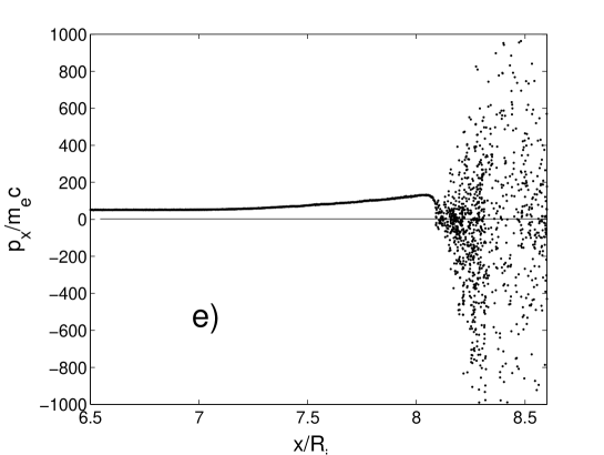
Figure 1: Electron and ion phase space and electromagnetic fields at $t=1.9R_{i}$; the initial Lorentz factor $\Gamma_{0}=50$, the magnetization $\sigma_{i}=0.003$, the ion-electron mass ratio $M/m=200$. a) longitudinal momentum of ions; b) longitudinal momentum of electrons at the front of the shock; c) electron phase space at the front of the shock, $8.088<x/R_{i}<8.101$; d) magnetic field; e) longitudinal momentum of electrons

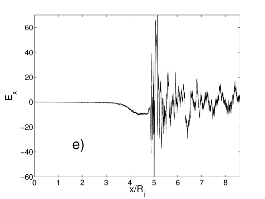
Figure 2: Electron and ion phase space and electromagnetic fields at $t=8.2R_{i}$. Parameters are the same as in Fig.1. a) longitudinal momentum of ions; b) longitudinal momentum of electrons; c) transverse momentum of electrons; d) magnetic field; e) longitudinal electric field

At $t=0$ the computation box is filled with a homogeneous plasma moving to the right with the Lorentz factor $\Gamma_{0}=(1-V_{0}^{2})^{-1/2}$. The thermal velocity dispersion is negligible. The plasma initially carries a uniform magnetic field, $B_{0}$, as well as the electric field $E_{x}=V_{0}B_{0}$. The flow moves to the right against a wall from which the particles are elastically reflected. The plasma is continuously injected from the left boundary. The condition of no incoming waves was adopted at the right boundary. In Figs. 1 and 2, the simulation results are presented for a run with the initial Lorentz factor of the flow $\Gamma_{0}=50$ and the ion-to-electron mass ratio $m_{i}/m_{e}=200$. The flow is weakly magnetized, $\sigma_{i}=0.003$. The system grid size is $204,000$, the particle density is 2 per species per cell, the time-step, $\Delta t=\Delta x$, was chosen such that $eB_{0}\Delta t/mc=0.5$. The length is measured in units of the upstream relativistic ion Larmor radius, $R_{i}=M\Gamma_{0}/eB_{0}$. The physical system size is $8.6R_{i}$.

According to the simulation results, a shock arises initially at the right boundary and then moves to the left. Fig. 1 shows the initial stage when the shock was just formed. One can see a well-developed ion loop in Fig. 1a. The front of the shock occurs when the upstream flow meets the first reflected ions ($x=8.01R_{i}$ at the presented snapshot). The electron flow near this point is shown in Fig. 1b; one can see that the electrons enter the shock non-adiabatically and that their motion becomes rotational. The ring formed in the electron phase space is clearly seen in Fig. 1c. Just below this initial region, the phase space hole disappears because the synchrotron instability develops and electron distribution spreads. Waves generated by the instability are clearly seen in Fig. 1d. The electromagnetic precursor propagates ahead of the shock front exciting oscillations of electrons and making the electrons lag behind the ions. A large-scale longitudinal electric field arises, which accelerates electrons. This acceleration is seen in Fig. 1e. The electrons start to accelerate when the precursor reach them (at $x=6.8R_{i}$ in the presented snapshot). At this stage, the electron energy gain is not large and the electrons enter the shock with an energy still much less than the energy of ions.

In the course of time, the shock propagates farther to the left and so does the precursor. As the electrons with a larger energy enter the shock, the amplitude of the precursor increases. In the wave with a larger amplitude, the electron guiding center slows down, a larger longitudinal electric field develops and, according to Eq.(20), the electrons acquire larger energy. When these new electrons enter the shock, they emit even stronger waves and then the energy of electrons in the upstream flow increases even more. The ion energy decreases appropriately because the total energy of the flow is conserved. Eventually, long-wavelength electrostatic oscillations develop. In these oscillations, the average energies of electrons and ions are equal. Fig.2 shows the simulation results at $t=8.2R_{i}$. Here the shock front is at $x=5R_{i}$. The shock is sharp, the shock width is of the order of $R_{i}$. Strong high frequency oscillations of the magnetic field at $0.5<z<5$ (see Fig.1d) represent the electromagnetic precursor. Downstream of the shock, the plasma density and the mean magnetic field are 3 times those upstream as they should be in a two-dimensional relativistic gas with a ratio of specific heats $3/2$ (note that all quantities are measured in the downstream frame; in the shock frame, the density jump is 2).

These simulations show that the energy equipartition between electrons and ions is achieved before the plasma enters the shock front so that downstream of the shock, the temperatures of ions and electrons are equal. The front of the precursor was emitted when the electrons with the initial Lorentz factor entered the shock; therefore the wave amplitude is initially not very large and the electrons are accelerated slowly but the amplitude grows when the electrons with larger energies enter the shock and therefore the precursor amplitude grows and the electrons are accelerated more rapidly. When the electrons achieve equipartition with ions, the amplitude of the precursor becomes maximal. At this stage, the precursor is taking few per-cent of the total energy of the flow.

The electrons at the shock front emit electromagnetic waves both forward and backward. In weakly magnetized flows, $\sigma_{i}\lesssim 0.01$, the energy density of the waves downstream of the shock exceeds that of the shock-compressed background magnetic field.

We ran simulations with the Lorentz factor of the flow from 2 to 50. It was found that electrons efficiently take energy from ions provided the flow is highly relativistic, $\Gamma_{0}>10$. In the mildly or non relativistic case, the shock does not emit waves strong enough to make electrons lag behind ions, so no longitudinal electric field arises.

There is no sign of nonthermal particle acceleration in these simulations; downstream of the shock, the distribution functions of both electrons and ions are Maxwellian. One of the reasons is that in the one-dimensional simulations, the electric field is orthogonal to the magnetic field. The Fermi acceleration presumably occurs at much larger scale and anyway requires three-dimensional turbulence. However this study shows that the nonthermal tail in the electron spectrum would begin, provided it forms, from the energy of the order of the upstream ion energy.

6 Discussion

It has been demonstrated in this paper that the maser instability develops at the front of the ultrarelativistic shock and generates electromagnetic waves propagating both upstream and downstream of the shock. Interaction of the upstream plasma flow with these waves results in efficient energy exchange between ions and electrons so that the energy equilibration occurs in the upstream flow before it arrives at the shock front. An important point is that the energy of the maser radiation is generally proportional to the energy of electrons entering the shock. Therefore eventually a few percent of the total energy of the flow is radiated away in the form of low-frequency waves.

Non-linear interactions of these waves with the plasma particles could significantly affect the process of particle acceleration. This issue demands multi-dimensional study and therefore is beyond the scope of the present work. In any case, electron-ion equilibration facilitates any acceleration process.

If the magnetization of the upstream flow is low, $\sigma<10^{-2}$, the energy density of waves downstream of the shock exceeds that of the shock-compressed background field. Relativistic particles could radiate in the field of the waves via nonlinear Compton scattering (e.g., Melrose 1980, pp. 136-141). The power and characteristic frequencies of this emission are similar to those for synchrotron emission in the magnetic field of the same strength as the wave amplitude. Therefore the overall spectrum of radiation from electrons with a power-law energy distribution generally mimics the synchrotron spectrum. However, there are marked differences. For example in the low-frequency range, $\omega\ll(eE_{0}/m_{e}c)\gamma^{2}$, the radiation spectrum of the nonlinear Compton scattering exhibits a larger slope than the synchrotron spectrum, $F_{\omega}\propto\omega$ (He et al. 2003) instead of the customary $F_{\omega}\propto\omega^{1/3}$.

Note that a good fraction of the gamma-ray bursts (GRBs) exhibit X-ray spectra growing faster than $\omega^{1/3}$ (Preece et al. 1998). There is still no conventional explanation of this fact (Lloyd & Petrosian 2000; Medvedev 2000, 2006; Mészáros & Rees 2000; Fleishman 2006) The presented model could naturally account for this behavior if one attributes the GRB emission, at least partially, to the nonlinear Compton scattering of low-frequency waves generated by the synchrotron maser at the shock front. Note also that observations of GRB afterglows suggest (Waxman 1997; Frail, Waxman & Kulkarni 2000; Eichler & Waxman 2005) that the electrons gain a significant fraction of the total energy such that their average energy is comparable with that of the ions. The present study shows that electrons indeed take about one-half of the total energy, which makes it relatively easy for any acceleration process to transfer a significant fraction of this energy to a nonthermal tail.

I am grateful to David Eichler and Anatoly Spitkovsky for valuable discussions. This research was supported by the grant I-804-218.7/2003 from the German-Israeli Foundation for Scientific Research and Development.

Appendix. Synchrotron instability

Let us assume that all electrons rotate in the magnetic field with the Lorentz factor $\Gamma\gg 1$. Such a plasma is evidently unstable with respect to maser synchrotron emission. The growth rate of the instability is maximal for the electromagnetic wave propagating perpendicularly to the magnetic field and polarized perpendicularly to the magnetic field; only this wave is considered here.

6.1 $\Omega_{B}\gg\Omega_{p}$

In this case one can neglect the influence of the plasma on the dispersion properties of the emitted waves. Then the growth rate of the synchrotron instability at the $j$-th harmonics is easily found as (e.g. Alexandrov, Bogdankevich & Ruhadze 1984, sect.6.4)

$$\kappa=\frac{\sqrt{3}}{2}\Omega_{B}\left[\frac{\Omega_{p}^{2}}{2\Omega_{B}^{2}j^{2}}J^{\prime 2}_{j}(jV)\right]^{1/3};$$

where $J_{j}$ is the Bessel function, $V=1-1/2\Gamma^{2}$ the electron velocity. The growth rate is maximal at the first harmonics, $\omega=\Omega_{B}=\Omega_{p}\sigma_{e}^{1/2}$, and may be written as

$$\kappa_{max}=0.3\sigma_{e}^{-1/3}\Omega_{B};\qquad\sigma_{e}\gg 1.$$

6.2 $\Omega_{B}\ll\Omega_{p}$

In this case only high harmonics of the gyrofrequency can propagate, and therefore be emitted, within the plasma. Then the maser instability develops only in the Rasin-Tsytovich range unless the electron ring is unrealistically narrow (McCray 1966; Zheleznyakov 1967). Sazonov (1970) and Sagiv & Waxman (2002) considered the maser instability of relativistic electrons with isotropic distribution in the case where the dispersive properties of the medium are determined by these electrons. In this section, a similar problem is solved for a ring-like distribution.

Making use of the Einstein coefficient method (e.g. Ginzburg 1989, ch.10) one can write the growth rate of the instability as the absorption coefficient with the opposite sign:

$$\kappa=\frac{8\pi^{3}c^{2}}{\omega^{2}}\sum A_{i}^{j}\left(N_{i}-N_{j}\right).$$

Here $N_{i}$ is the population of the $i$-th Landau level. Introducing the distribution function, $f(p_{\bot},p_{\|})$, normalized by the condition $\int fd\mathbf{p}=1$ and making use of the energy conservation in the emission process, one can write

$$N_{i}-N_{j}=N\frac{\partial f(p_{\bot},p_{\|})}{\partial p_{\bot}}\frac{\varepsilon}{p_{\bot}}\hbar\omega;$$

where $\varepsilon$ is the electron energy, and $p_{\bot}$, $p_{\|}$ are the components of the momentum perpendicular and parallel to the magnetic field. The Einstein coefficients, $A_{i}^{j}$, are straightforwardly expressed via the conventional formula for the power of the synchrotron radiation from a single electron, $q$; this yields

$$\kappa=\frac{4\pi^{2}cN}{\omega^{2}}\int q\frac{\partial f(p_{\bot},0)}{\partial p_{\bot}}p_{\bot}^{2}dp_{\bot};$$

$$q=\frac{3^{1/2}e^{2}\omega_{B}}{2c[1+\gamma^{2}(1-n^{2})]^{1/2}}\frac{\omega}{\omega_{c}}\left[\int_{\omega/\omega_{c}}^{\infty}K_{5/3}(z)dz+K_{2/3}\left(\frac{\omega}{\omega_{c}}\right)\right];$$

$$\omega_{c}=\frac{3}{2}\omega_{B}\gamma^{2}[1+\gamma^{2}(1-n^{2})]^{-3/2};$$

where $K_{j}$ is the Macdonald function, $n$ the refraction index of the medium and it was assumed that $\gamma\gg 1$ so that the electron radiates exactly in the direction of its motion. Integrating equation (A2) by parts, one gets

$$\kappa=\frac{\pi\omega_{p}^{2}m_{e}}{\sqrt{3}\omega}\int f(p_{\bot},0)\frac{\partial}{\partial p_{\bot}}\left\{p_{\bot}^{2}\left(n^{2}-1-\frac{1}{\gamma^{2}}\right)\left[\int_{\omega/\omega_{c}}^{\infty}K_{5/3}(z)dz+K_{2/3}\left(\frac{\omega}{\omega_{c}}\right)\right]\right\}dp_{\bot}$$

The refraction index of the wave propagating transversely to the magnetic field and polarized transversely to the magnetic field is expressed via the transverse dielectric permittivity as $n=\sqrt{\epsilon}$, where (e.g. Alexandrov et al. 1984)

$$\epsilon=1+\frac{\omega_{p}^{2}}{\omega}\int\frac{p_{y}}{\gamma(\omega-kv_{x})}\frac{\partial f}{\partial p_{y}}d\mathbf{p}.$$

For a narrow relativistic ring with the distribution function

$$f(p_{\bot},p_{\|})=\frac{1}{4\pi^{2}m_{e}^{3}\Gamma(\delta\Gamma)^{2}}\exp\left(-\frac{(p_{\bot}-m_{e}\Gamma)^{2}+p_{\|}^{2}}{2(\delta\Gamma)^{2}}\right);$$

where $\delta\Gamma\ll\Gamma$, one finds

$$\epsilon=1+\frac{\Omega_{p}^{2}}{k^{2}}\left\{1-\sqrt{1-\frac{k^{2}V^{2}}{\omega^{2}}}-\frac{k^{2}V^{2}}{\omega\Gamma^{2}\sqrt{\omega^{2}-k^{2}V^{2}}}\right\}.$$

In the case $\omega\gg\Omega_{p}$ so that $n-1\ll 1$, the refraction index takes the usual form

$$n^{2}=1-\frac{\Omega_{p}^{2}}{\omega^{2}}.$$

In the Rasin-Tsytovich regime, $\Gamma^{2}(n^{2}-1)\gg 1$, equation (A3) yields for the distribution function (A4)

$$\kappa=\frac{\Omega_{p}^{4}\Gamma}{\sqrt{6\pi}\omega^{3}\delta\Gamma}F\left(\frac{2\Omega_{p}^{3}}{3\Omega_{B}\omega^{2}}\right);$$

where

$$F(z)=zK_{5/3}(z)-\int_{z}^{\infty}K_{5/3}(x)dx-(4/3)K_{2/3}(z).$$

The function $F(z)$ achieves its maximum at $z=2.2$ and its maximal value is 0.085. Now one can estimate the maximal growth rate of the instability as

$$\kappa_{max}=0.1\frac{\Gamma}{\delta\Gamma}\Omega_{B}\sigma_{e}^{1/4};\qquad\sigma_{e}\ll 1.$$

The corresponding emission frequency is $\omega=0.5\Omega_{p}\sigma_{e}^{-1/4}$.

References

- (1) Alexandrov, A.F., Bogdankevich, L.S. & Rukhadze A.A. 1984, Principles of plasma electrodynamics (Berlin: Springer-Verlag)
- (2) Birdsall, C.K. & Langdon, A.B. 1991, Plasma physics via computer simulation (London: IOP Publishing)
- (3) Bingham, R., Kellett, B. J., Cairns, R. A., Tonge, J. & Mendonça, J. T. 2003, ApJ 595, 279
- (4) Eichler D. & Waxman E. 2005, ApJ 627, 861
- (5) He, F., Lau, Y. Y., Umstadter, D.P. & Kowalczyk, R. 2003, Phys.Rev.Lett. 90, 5002
- (6) Frail D.A., Waxman E. & Kulkarni S.R. 2000, ApJ 537, 191
- (7) Gallant, Y.A.,Hoshino, M.; Langdon, A.B. Arons, J. & Max, C.E. 1992, ApJ 391, 73
- (8) Ginzburg, V.L. 1989, Application of electrodynamics in theoretical physics (New York: Gordon and Breach)
- (9) Hoshino M., Arons, J., Gallant, Y.A. & Langdon, A. B. 1992, ApJ 390, 454
- (10) Hoshino, M. & Shimada, N. 2002, ApJ 572, 880
- (11) Landau L.D. & Lifshitz E.M. 1995, The classical theory of fields (Butterworth-Heinemann: Oxford [England])
- (12) Langdon A.B., Arons J. & Max C.E. 1988, Phys. Rev.Lett., 61, 779
- (13) Lloyd, N. M. & Petrosian, V. 2000, ApJ 543, 722
- (14) McClements, K. G., Dieckmann, M. E., Ynnerman, A., Chapman, S. C., & Dendy, R. O. 2001, Phys. Rev. Lett., 87, 255002
- (15) McCray, R. 1966, Sci 154, 1320
- (16) Medvedev, M. V. 2000, ApJ 540, 704
- (17) Medvedev, M. V. 2006, ApJ 637, 869
- (18) Mészáros, P. & Rees, M. J. 2000, ApJ 530, 292
- (19) Preece et al. 1998, ApJ 506, L23
- (20) Sagiv, A. & Waxman, E. 2002, ApJ 574, 861
- (21) Sazonov, V. N. 1970, Soviet Astron.AJ, 13, 797
- (22) Shimada, N. & Hoshino, M. 2000, ApJ 543, L67
- (23) Schmitz, H., Chapman, S. C. & Dendy, R. O. 2002a, ApJ 570, 637
- (24) Schmitz, H., Chapman, S. C. & Dendy, R. O. 2002b, ApJ 579, 327
- (25) Tokar, R. L., Aldrich, C. H., Forslund, D. W. & Quest, K. B. 1986, Phys.Rev.Lett. 56, 1059
- (26) Zheleznyakov, V. V. 1967, Soviet Phys.JETP, 24, 381
- (27) Waxman E. 1997, ApJ 489, L33