Capturing the Fire: Flame Energetics and Neutronizaton for Type Ia Supernova Simulations

Abstract

We develop and calibrate a realistic model flame for hydrodynamical simulations of deflagrations in white dwarf (Type Ia) supernovae. Our flame model builds on the advection-diffusion-reaction model of Khokhlov and includes electron screening and Coulomb corrections to the equation of state in a self-consistent way. We calibrate this model flame—its energetics and timescales for energy release and neutronization—with self-heating reaction network calculations that include both these Coulomb effects and up-to-date weak interactions. The burned material evolves post-flame due to both weak interactions and hydrodynamic changes in density and temperature. We develop a scheme to follow the evolution, including neutronization, of the NSE state subsequent to the passage of the flame front. As a result, our model flame is suitable for deflagration simulations over a wide range of initial central densities and can track the temperature and electron fraction of the burned material through the explosion and into the expansion of the ejecta.

1. Introduction

Type Ia supernovae (SNe) are bright explosions characterized by strong silicon P Cygni features near maximum light and a lack of hydrogen spectral features. The currently favored interpretation is the disruption of a near-Chandrasekhar-mass C/O white dwarf by a thermonuclear runaway (for a review, see Hillebrandt & Niemeyer, 2000, and references therein). These events are fascinating in and of themselves and are important both for their contribution to the cosmic abundance of iron-peak elements and for their role as standard candles.

Models of Type Ia SNe necessarily involve a mechanism for incinerating the star by a thermonuclear runaway, and the nature of this mechanism is the subject of contemporary research. In the explosion, a thermonuclear flame propagates through the C/O fuel of the white dwarf as either a subsonic deflagration front (Nomoto et al., 1976, 1984; Reinecke et al., 2002; Gamezo et al., 2003) or a supersonic detonation wave (Arnett, 1969; Boisseau et al., 1996) and releases sufficient energy to unbind the star. However, models involving either a pure deflagration or a pure detonation have traditionally been unable to provide an explanation for both the observed expansion velocities and the spectra produced by ejecta that are rich in intermediate-mass and iron-peak elements (Truran & Cameron, 1971; Woosley & Weaver, 1986; Petschek, 1990). Recent work, however, suggests that a fast deflagration alone may provide sufficient energy to unbind the star (Hillebrandt & Roepke, 2005).

There has been considerable progress recently in hydrodynamical simulations of deflagrations of C/O white dwarfs (Röpke & Hillebrandt, 2005; Gamezo et al., 2005) that model the entire star. This is a complicated endeavor, predominantly due to the vast range of length scales: the laminar flame width is $\sim 10^{-3}\textrm{--}10\,\mathrm{cm}$, some 8 to 12 orders of magnitude smaller than the stellar radius (Timmes & Woosley, 1992). Because the computational requirements for simulations with these disparate scales demand resources well beyond current capabilities, multidimensional Type Ia models must make use of an appropriate sub-grid-scale model for the evolution of the thermonuclear burning front. Moreover, large-scale simulations are very demanding of computational resources, and it is not feasible at present to include enough nuclides to allow for directly computing the reaction kinetics. A realistic model must accurately describe the nuclear energy that is released, the timescale on which it is released, and the compositional changes that occur in the flame. In addition, the burned material continues to evolve after the passage of the flame due to both weak interactions and hydrodynamic evolution, and realistic simulations must describe this “post-flame" evolution.

In this paper we present a study of the nuclear burning that occurs during C/O deflagrations, with the goal of producing a realistic flame model for simulations of Type Ia supernovae. Building on the advection-diffusion-reaction (ADR) flame model of Khokhlov (1995), we further develop a three-stage flame model. The work described here improves upon earlier calculations in several ways. First, screening and the Coulomb interaction are included self-consistently in the forward and inverse rates, so that detailed balance is preserved. Second, we account for the neutronization and neutrino loss rates via electron captures at high densities. Our treatment is sufficiently general that it can also describe the expansion following the explosion. With minimal tuning, the method should capture the bulk energetics and associated “freezing" of the abundance pattern as the matter expands.

The present paper is concerned with describing with the utmost care the nuclear processes that occur in the real flame and proposing a method that can capture the necessary features: energy release, its timescales and neutronization. The hydrodynamic behavior in the 3-dimensional flow (importance of flame front curvature, acoustic behavior, flame front stability, effects of finite resolution, etc.) is under active investigation. Due to the complexity of those issues, the fact that the work is still in progress, and the clean separation of much of them from the nuclear physics addressed here, we have chosen to publish this work in advance of a forthcoming separate hydrodynamical study. It is important to note that such a hydrodynamical study must be performed in order to understand how this particular flame-capturing technique, with realistic energetics, behaves in simulations of a deflagration in a WD.

Our three-stage flame model describes the propagation of a nuclear flame through a uniform $\mathrm{{}^{12}C}$/$\mathrm{{}^{16}O}$ mixture. In this work we consider the case of a mixture with 1:1 mass fractions, but the method can be applied to any ratio. As described in Khokhlov (2000), the burning occurs in roughly three stages with well-defined timescales. First is the $\mathrm{{}^{12}C}+\mathrm{{}^{12}C}$ fusion, leading to a mixture consisting of the unburned $\mathrm{{}^{16}O}$ together with $\mathrm{{}^{20}Ne}$, $\mathrm{{}^{24}Mg}$, and $\alpha$-particles. Second, the resulting mix burns on a longer timescale leading to the formation of predominantly Si-group (intermediate mass) $\alpha$-elements and $\alpha$-particles, a state that is commonly referred to as nuclear statistical quasi-equilibrium (NSQE). Third, these elements burn on a still longer timescale to nuclear statistical equilibrium (NSE), which at the densities of interest in the deflagration phase of Type Ia SNe, consists primarily of Fe-peak nuclei, $\alpha$-particles, and protons.

After the flame has burned the C/O fuel, two factors continue to influence the energetics: (1) decreases (or possibly increases) in temperature and density resulting from the large-scale motion of the star, and (2) neutronization of the hot nuclear ash. Neutronization can heat or cool the ash, depending on whether the nuclear binding energy released by neutronization exceeds or falls short of the energy lost by neutrinos, and the competition between these two processes is a sensitive function of density. We note that because the light curves of SNe Ia are strongly sensitive to the mass of ⁵⁶Ni produced, the degree to which neutronization reduces the mean ⁵⁶Ni concentration over the regions of the core (extending out to $\approx$ 0.8-1 M_⊙) in which conditions of nuclear statistical equilibrium are achieved is clearly a critical issue. It is therefore important to provide an accurate measure of the influence of electron captures on the energetics. Only in this way can we ensure that the peak temperatures and temperature histories of fluid elements are accurate. Accordingly, our flame model follows this neutronization.

In this paper we describe nuclear flame propagation (§ 2). We describe fully-resolved simulations of thermonuclear flames propagating through a slab of stellar material and compare these to similar “one-zone" simulations of nuclear burning. The “one-zone" or “self-heating" simulations allow for a longer-time evolution than the fully-resolved flames and provide the energetics and timescales for the model flame. Comparison to the fully-resolved flame calculations is an important consistency test. In this section we also describe the method by which we determine the density contrast across the flame as is required as input by the flame model and present contrasts at selected densities measured from the fully-resolved flame simulations. In (§ 3) we describe our model flame. We outline the basics of our ADR flame capturing scheme and describe the stages of nuclear burning and the energy release occurring in each. In (§ 4), we describe the calculations of energetics and timescales that serve as input to the flame model. We present the results of self-heating simulations of nuclear burning with a detailed nuclear reaction network and contemporary reaction rates. We report on the effect of including Coulomb corrections and screening and present timescales for burning to NSQE and NSE. In (§ 5), we describe the change in energy resulting from the evolution of the burned material in NSE. We present a study of the NSE state that quantifies the change in binding energy with temperature and density evolution and the effects of weak interaction (neutronization). We also describe our method of representing the NSE state with a reduced set of nuclei. In (§ 6) we present results of model flame simulations at several densities, and in (§ 7) we draw conclusions from this effort. Finally, we present an appendix with details of the plasma coulomb corrections applied to both the network and NSE calculations.

2. Nuclear Flame Propagation

A thermonuclear flame in the interior of a star propagates subsonically. This slow propagation makes following the flame with an explicit hydrodynamics method such as PPM difficult because of the high spatial resolution needed to resolve the flame. The time step in an explicit hydrodynamics method is limited by the Courant condition; namely, the code must resolve the sound-crossing time of the smallest zone. Because of this constraint, the time steps for a high-resolution simulation are very small and a large number of time steps is therefore required to propagate the subsonic flame, even across just a few simulation zones. This problem is particularly acute at lower densities for which the timescale for burning is relatively long. A fully-resolved flame simulation could literally take billions of time steps, which is impractical and would most likely produce inaccurate results. We implement the flame model in the explicit hydrodynamics code flash (Fryxell et al., 2000; Calder et al., 2002), but rely for input to the model flame on self-heating network calculations described in this section.

2.1. Nuclear Flame Structure and Self-Heating Calculations

Because of the difficulty encountered with propagating flames with flash, particularly at low densities, we made use of self-heating network calculations (see section 4 for details). These are (energetically) closed-box calculations of nuclear burning at either constant pressure (isobaric) or constant density (isochoric). We use both cases in this paper, each for a different purpose. Isobaric behavior should be quite close to what occurs in a fluid element as the subsonic flame sweeps through it, so that, in a sense, such a self-heating network calculation may be thought of as a “one-zone" calculation. Isochoric calculations are thermodynamically simpler and for this reason are used in section 4 to gauge the effects of screening and to compare different reaction networks. As will be shown below, the results of isobaric and isochoric calculations are fairly similar for high density ($\rho>10^{8}$ g cm^-3).

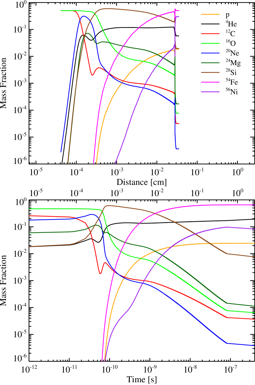
Figure 1.— Top panel: Results from a fully resolved DNS of a propagating flame at $10^{9}\ \mathrm{g\ cm^{-3}}$ performed with flash and the aprox19 network. Shown are abundances for p, $\mathrm{{}^{4}He}$, $\mathrm{{}^{12}C}$, $\mathrm{{}^{16}O}$, $\mathrm{{}^{20}Ne}$, $\mathrm{{}^{24}Mg}$, $\mathrm{{}^{28}Si}$, $\mathrm{{}^{54}Fe}$, and $\mathrm{{}^{56}Ni}$ plotted against the distance from the flame position so that the flame is propagating to the left. The small “tails" at the right are artifacts of the “match head" used to ignite the flame. The simulation was run on an adaptive mesh with an effective resolution of $7.81\times 10^{-6}\mathrm{cm}$. Bottom panel: Results from an isochoric simulation at $10^{9}\ \mathrm{g\ cm^{-3}}$ performed with the self-heating 19 nuclide network aprox19. Shown are the same abundances as the top panel plotted against the time and the calculated distance. The distance scaling along the top axis was obtained by multiplying the time by the flame speed with respect to the (expanded) ash.

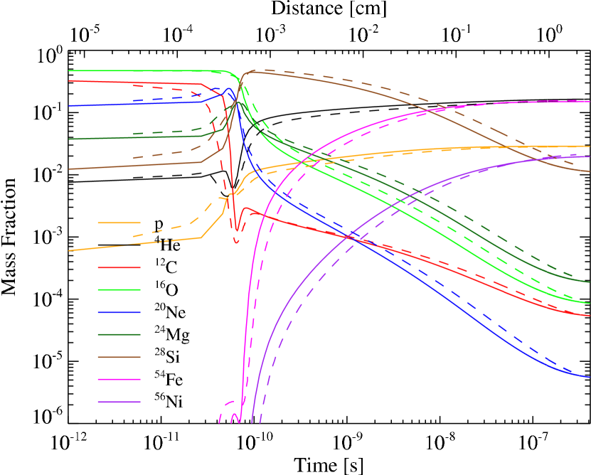
Figure 2.— Abundance evolution of burning an equal-mass mix of C and O from an initial density of $10^{9}\ \mathrm{g\ cm^{-3}}$. Shown are the results from a isochoric (solid lines) and an isobaric ($P=5\times 10^{26}$ dyne cm^-2; dashed lines) self-heating calculation. Our 200 nuclide network was used in both calculations. The approximate distance scale is as in Fig. 1.

We refer to an actual propagating flame simulated with flash using thermal diffusion as a direct numerical simulation (DNS). An important test is the consistency between actual flames propagated with flash and the results of the self-heating calculations. We performed simulations of propagating flames with flash at several relatively high densities for which a flame calculation was feasible. The most notable difference between the DNS and the self-heating calculations is that it is necessary to use a fairly small reaction network (19 nuclides) in the DNS, whereas the self-heating calculations are able to use a much larger network (200 nuclides, see section 4). The DNS employed adaptive mesh refinement with an effective resolution of $7.81\times 10^{-6}\mathrm{cm}$. The minimum refinement of the mesh was kept at $1.56\times 10^{-5}\mathrm{cm}$, and one additional level of AMR allowed the extra resolution of the flame front.

A comparison of a DNS and isochoric self-heating is shown in Fig. 1. Both of these calculations use the 19 nuclide network aprox19 (Weaver et al., 1978; Timmes, 1999) to burn fuel which is initially an equal mass mixture of $\mathrm{{}^{12}C}$ and $\mathrm{{}^{16}O}$ at a density of $10^{9}\ \mathrm{g\ cm^{-3}}$. The top panel shows how abundances vary with distance behind the flame front in the DNS (so that unburned material is on the left). The flame was ignited at the edge of a 0.08 cm domain by raising the temperature of a small region of the domain to the unphysically high value of $10^{10}$K. Heat then diffuses from this preheated region and ignites the flame, which then propagates across the grid. The rightmost parts of the mass fraction curves, at the largest distance from the flame, have small “tails” that result from the unphysical initial conditions of the very hot “match head.” Shown are mass fractions for p, $\mathrm{{}^{4}He}$, $\mathrm{{}^{12}C}$, $\mathrm{{}^{16}O}$, $\mathrm{{}^{20}Ne}$, $\mathrm{{}^{24}Mg}$, $\mathrm{{}^{28}Si}$, $\mathrm{{}^{54}Fe}$, and $\mathrm{{}^{56}Ni}$. The flame speed calculated from this simulation, $34.2\ \mathrm{km\ s^{-1}}$, agreed well with the result of Timmes & Woosley (1992).

The abundance evolution with time from an isochoric self-heating calculation using the same network is shown in the bottom panel of Fig. 1. We have calculated an approximate distance from the flame front (shown on the upper scale) by multiplying the time by the flame speed with respect to the ash. From conservation of mass this is related to the laminar flame speed in the fuel by $S_{\rm ash}=S_{\rm lam}(1+A)/(1-A)$, where $A=(\rho_{\rm fuel}-\rho_{\rm ash})/(\rho_{\rm fuel}+\rho_{\rm ash})$ is the Atwood number. For this calculation we used values of $A_{\rm P200}$ in Table 1 (see description in § 2.2) and the laminar flame speed from Timmes & Woosley (1992), $S_{\rm lam}=5.3\times 10^{6}~{}{\rm cm\,s^{-1}}$ for $\rho=10^{9}\ \mathrm{g\ cm^{-3}}$ and $X(\mathrm{{}^{12}C})=0.5$ (see eq. [5]). We find good agreement in terms of abundance structure between the isochoric self-heating calculation and DNS. The stretching on the left in the bottom panel is due to the choice of zero point. With an initial temperature $T=1.7\times 10^{9}~{}{\rm K}$, there is a long smoldering phase in the self-heating calculation before rapid consumption of $\mathrm{{}^{12}C}$ occurs. The same "pre"-heating is accomplished in the DNS by thermal diffusion, giving a heating time and length scale similar to the $\mathrm{{}^{12}C}$ consumption scales. To be able to broaden the region where C/O decreases sharply, we chose the time zero to be a time where C/O starts to decrease. Since the C consumption timescale is short compared to the later flame stages (e.g. reaching NSE), this choice does not affect the total flame thickness. Also the depletions of $\mathrm{{}^{12}C}$ and $\mathrm{{}^{16}O}$ are shifted slightly further in distance in the self-heating plot by our use of a constant distance scaling because this is in reality where the expansion takes place.

The next step is to compare these results with those of the much larger nuclear network that will be used for the rest of our self-heating calculations. Fig. 2 shows the abundance evolution for $\rho=10^{9}$ g cm^-3 using the 200 nuclide network described in § 4. The two networks give very similar evolutions, with the most notable difference being in the final abundances. The 200 nuclide network has many more nuclides available near the Fe peak, such that less material is concentrated in a single nuclide (⁵⁴Fe) than with the small network. The 5 most abundant nuclides in the NSE state are ⁵⁴Fe, ⁴He, ⁵⁵Co, ⁵⁸Ni, ⁵⁶Co with abundances of 16%, 13%, 8.4%, 7.3% and 6.2% respectively, and there are another 14 nuclides with abundances between 1 and 5%.

The evolution of a fluid element as the subsonic flame passes is in fact nearly isobaric. Due to the high level of degeneracy at $\rho=10^{9}$ g cm^-3, however, there is little expansion and so the isochoric and isobaric self-heating calculations give quite similar results. In Fig. 2, we also show the result from an isobaric calculation. Here the pressure ($P=5\times 10^{26}~{}{\rm dynes\,cm^{-2}}$) is chosen to give an initial density of $10^{9}$ g cm^-3. We can see that the isobaric calculation takes slightly longer to reach NSQE, a result of a slightly decreased temperature due to expansion. The density is decreased to $8.3\times 10^{9}\ \mathrm{g\ cm^{-3}}$ at this phase. However, the NSE timescale and the final NSE abundances don’t differ much from the isochoric calculation.

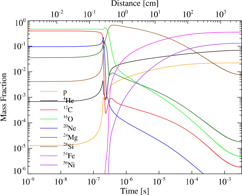
Figure 3.— Similar to Fig. 2 but for isobaric only with an initial density of $10^{8}\ \mathrm{g\ cm^{-3}}$.

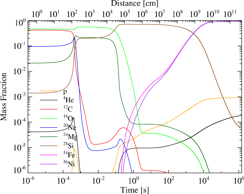
Figure 4.— Similar to Fig. 2 but for isobaric only with an initial density of $10^{7}\ \mathrm{g\ cm^{-3}}$.

Before discussing the general features of this flame structure, it is useful to see how it changes when burning at lower densities. Figs. 3 and 4 show isobaric self-heating calculations for initial densities of $\rho_{i}=10^{8}$ and $10^{7}$ g cm^-3. Light particles, particularly $\alpha$-particles, become less dominant in the NSE final state. It is already evident that at these low densities the flame becomes very extended physically, such that a profile like that shown in Fig. 4 could never be realized in an actual star. The dynamical response time of the star is shorter than these timescales (see Fig. 11), causing the reactions to freeze out due to expansion, and the scale height at this density is smaller than the large scales of the structure shown.

At all densities, though the overall progression timescale differs significantly, the three burning stages are evident. Beginning with equal parts by mass of ¹²C and ¹⁶O, initially the burning of the ¹²C leads to a mixture of ¹⁶O, ²⁰Ne, ²⁴Mg, and $\alpha$-particles. This mixture then burns to intermediate mass (²⁸Si to ⁴⁰Ca) nuclei and $\alpha$-particles (NSQE) in which most of the energy release has taken place. Finally, the mixture reaches full NSE consisting of a temperature and density dependent mixture of iron-peak nuclei, $\alpha$-particles, and protons. The transition points at $\rho=10^{8}$ g cm^-3 (Fig. 3) are at 0.2, 0.4, and 30 cm on the approximate distance scale. While the ¹²C burning and the transition to NSQE are well separated at the low density, at the higher densities these stages appear more as an offset between consumption of ¹²C and ¹⁶O.

It is important to note again that the NSE state is not static. The forward and inverse rates are large but balanced, which enables the NSE state to adjust as the fluid element evolves under hydrodynamical motions (see § 5 for further details). The flame model must reproduce this behavior with good approximations to the flame propagation speed, energy release timescales, and total energy release.

2.2. Inferring Density Contrast From Isochoric Calculations

In the flamelet regime, the flame is accelerated by the Rayleigh-Taylor instability, which increases the surface area of the flame and its effective propagation speed (Khokhlov, 1995; Niemeyer & Kerstein, 1997). The strength of this effect is related to the density contrast, characterized via the Atwood number, $A$, due to the energy release in nuclear burning. Energy is released and does work to expand the matter and raises the temperature until NSE is reached (for densities $\gtrsim 10^{7}\ \mathrm{g\ cm^{-3}}$) or the nuclear energy is exhausted upon fusion to $\mathrm{{}^{56}Ni}$.

The energy release found from an isochoric self-heating calculation can be used to estimate the expansion expected for the actual (approximately isobaric) burn. We denote this approximate Atwood number by $\tilde{A}$, and calculate it by using a single-stage ADR flame (see Section 3.1) that has a specified energy release, $\Delta Q$, and ash composition taken from an isochoric self-heating calculation (these are given in Table 3). The ash composition defines both the heat capacity and the relationship between the ion pressure contribution and the temperature. Table 1 compares Atwood numbers calculated using high-resolution DNS of flames, $A_{\rm DNS}$, as was shown in Fig. 1, and $\tilde{A}$ for isochoric self-heating calculations computed with two reaction networks, aprox19 and P200. By comparing these three cases we can see what differences are due to the nuclear network alone, and what are due to the isochoric approximation. Self-heating calculations with the aprox19 nuclear network, the same as that used in the DNS, give a larger total energy release at the high densities relative to those found using our 200 nuclide network (see column 5), which is reflected in $\tilde{A}$ (column 3 and 4).

The approximate Atwood numbers, $\tilde{A}$, are lower than the actual Atwood numbers. The ash temperatures, $\tilde{T}_{\rm ash}$, found for the P200 case in this approximate scheme are shown in column 6, and are lower than the final temperatures (shown in Table 3) of the self heating calculations from which the $\Delta Q$ was drawn, reflecting the fact that some of the energy was used to do work for the expansion. This lower temperature means that the ash is now out of NSE, and if allowed to relax it would release nuclear binding energy, expand, and raise its temperature to reach the $A$ found in the DNS.

We find that, at these densities ($\rho>10^{8}$ g cm^-3), isochoric self-heating calculations provide reasonable estimates for the expansion factor and very gross estimates for the energy release. From this we conclude that $\tilde{A}$ from the isochoric self-heating calculation can be used as a static approximation where needed. We should emphasize, however, that in the model flame described below, the actual total energy release of the flame is determined by the NSE in post-flame material, which is calculated dynamically as described in section 5, and therefore will reproduce that of an isobaric flame.

Table 1Atwood numbers

density	$A_{\rm DNS}$	$T_{\rm ash\;DNS}$	$\tilde{A}_{\rm aprox19}$	$\tilde{A}_{\rm P200}$	$\Delta Q_{\rm aprox19}-\Delta Q_{\rm P200}$	$\tilde{T}_{\rm ash}$
($10^{9}\ \mathrm{g\ cm^{-3}}$)		$10^{9}\ \mathrm{g\ cm^{-3}}$)			(10${}^{17}\ \mathrm{erg\ g^{-1}}$)	(109 K)
6	0.065	10.5	0.056	0.051	0.21	6.7
2	0.093	9.34	0.082	0.077	0.15	6.8
1	0.116	8.51	0.101	0.097	0.08	6.6
0.5	0.150	7.80	0.127	0.125	0.05	6.3
0.1			0.227	0.229	-0.06	5.3

3. Implementation of Model Flame Energetics

The key ingredient in numerical simulations of the deflagration phase of SNe Ia is the nuclear flame model. In this section we describe our flame model, the implementation of the energetics, and the implementation of the “post flame" NSE evolution.

3.1. Basics of an ADR Flame model

Figure 5.— flame front structure for a one-stage ADR flame

We use a flame-capturing scheme based on the ADR method (Khokhlov, 1995, 2000) that is described in detail in Vladimirova et al. (2006). The flame front is localized via the value of a reaction progress variable, $\phi$, such that in the reactant $\phi=0$, in the product $\phi=1$, and $\phi$ varies monotonically across the flame front (see Fig. 5). The width of the ADR flame is often much larger than the thickness of the physical flame it represents, as it is prescribed to be several computational zones thick, thereby becoming even kilometers in width in full-star supernova simulations. The value of $\phi$ is defined everywhere on the grid, and can be associated with the mass fraction of burned material in a cell, provided that the reactant composition is initially uniform.

The reaction progress variable is evolved via an advection-diffusion-reaction equation,

$${{\partial\phi}\over{\partial t}}+{\bf v}\cdot\nabla\phi=\kappa\nabla^{2}\phi+\frac{1}{\tau}R(\phi)~{},$$ (1)

with artificial reaction and diffusion coefficients

$$\kappa={\rm const},\qquad R(\phi)=\left\{\begin{array}[]{ll}R_{0}={\rm const.,}&{\rm if}~{}~{}\phi_{0}\leq\phi\leq 1\\ 0,&{\rm otherwise,}\end{array}\right.\\$$ (2)

where $\phi_{0}$ marks the value of $\phi$ at which the reaction begins.

When $\bf{v}=0$, the solution of equation (1) is a traveling wave with speed $S_{0}$ with a specific functional form, $\phi(x-S_{0}t)$. Traveling speed $S_{0}$ and front thickness $l_{0}$ depend on the diffusivity, the reaction time, and the amplitude of the reaction rate, $S_{0}\propto\sqrt{R_{0}\kappa/\tau}$ and $l_{0}\propto\sqrt{\kappa\tau/R_{0}}$. For the reaction rate (2), the expressions for $S_{0}$ and $\phi(x-S_{0}t)$ can be found analytically. As shown in Vladimirova et al. (2006), if the amplitude of the reaction rate $R_{0}$ satisfies the relation $(\phi_{0}-R_{0})e^{1/R_{0}}+R_{0}=0$, the front propagates with the speed $S_{0}=\sqrt{\kappa/\tau}$. In our implementation, $\phi_{0}=0.3$ and $R_{0}=0.3128$, so the front speed and thickness obey the relations $S_{0}=\sqrt{\kappa/\tau}$ and $l_{0}=4\sqrt{\kappa\tau}$.

When $\bf{v}\neq 0$, the front propagates with the speed $S_{0}$ with respect to the background velocity, provided the velocity variations on the scale of the front thickness are negligible in comparison with $S_{0}$.

The ADR flame model uses the evolution of $\phi$ according to equation (1) to propagate a front. The front speed $S$ and the front thickness $l$ are input parameters; they determine the coefficients $\kappa$ and $\tau$ in equation (1),

$$\kappa=aSl/4,\qquad\tau=l/(4aS).$$ (3)

Here, $a$ is an adjustment coefficient that accounts for the front speed dependence on thermal expansion (since thermal expansion results in velocity variations across the front and alters the front speed). The coefficient $a$ depends on the density ratio $\alpha=\rho_{\mathrm{u}}/\rho_{\mathrm{b}}$ and, for the reaction rate (2), was estimated as $a=1+0.3(\alpha-1)\approx 1+0.6A$ (Vladimirova et al., 2006). Here $\rho_{\mathrm{u}}$ and $\rho_{\mathrm{b}}$ are the unburned and burned densities, respectively. Note that when $a=1$, we have $S=S_{0}$ and $l=l_{0}$. An empirical calibration was made based upon flames propagated with the multistage flame (described below), finding $a\approx 1+1.5A$. We attribute the difference to the energy release occurring in the second stage, slightly after the ADR flame front. The front thickness is set to be several grid points (spaced by $\Delta x$) per interface $l=b\Delta x$, usually with $b=4$. Further details of the implementation of this flame-capturing method may be found in Vladimirova et al. (2006).

The above description of the ADR flame capturing scheme describes the method of propagating a model flame at a specified speed. Flames passing through stellar material are subject to fluid instabilities, particularly the Rayleigh-Taylor instability, which increases mixing and therefore the effective flame speed. Analyzing the balance between generation and destruction of flame surface in a steady turbulent burning regime, Khokhlov (1995) showed that the flame surface packed in a given volume is inversely proportional to the laminar flame speed. Consequently, the total burning rate, which is equal to the product of the laminar flame speed and the flame surface area, is independent of the laminar flame speed in this regime. Numerical calculations of flames propagating in a vertical column demonstrate that the effective flame speed is determined by the large-scale motion rather than by the local flame properties (Khokhlov, 1995; Zhang et al., 2006). To account for flame acceleration on scales unresolved by the simulation, we use a turbulent subgrid flame speed (Khokhlov, 1995),

$$S_{\rm sub}=0.5\sqrt{Ag\Delta x},$$ (4)

where $g$ is the local gravitational acceleration. As an input to ADR model we take $S=\max(S_{\rm lam},S_{\rm sub})$, where the laminar flame speed,

$$S_{\rm lam}=9.2\times 10^{6}\,\left(\frac{\rho_{\mathrm{u}}}{2\times 10^{9}\ \mathrm{g\ cm^{-3}}}\right)^{0.803}\ \mathrm{cm\ s^{-1}},$$ (5)

is from Timmes & Woosley (1992).

The subgrid flame speed (eq. [4]) depends on the Atwood number $A$. To compute $A$ exactly, one must know the densities ahead of and behind the flame interface. The straightforward approach of “taking a probe” on both sides of the flame works well with models in which an infinitely-thin interface is reconstructed inside the computational cell and information about burned and unburned fluid is available in every partially burned cell. In the ADR flame model, to compute $A$ in the partially burned cell, one must “take a probe” at the location several computational cells away. It is not easy to develop a robust algorithm for locating pure fuel and pure ash in the vicinity of a particular partially burned cell. Efficiently implementing such an algorithm in a parallel, domain-decomposed simulation code such as flash is even more complicated because the information needed to perform the calculation for a given computational zone may not be directly available.

An alternate approach is to use local information to estimate the burned and unburned states from the partially burned state (Khokhlov, 1995; Vladimirova et al., 2006). The approach is based on the proportionality between the mass fraction of product $\phi$ and the fraction of energy released, so that the thermodynamical state can be parameterized by $\phi$. In particular, the density of the partially burned fluid can be obtained from the unburned state and $\phi$,

$$\rho=\frac{\rho_{\mathrm{u}}}{1+(\alpha-1)\phi},\qquad\alpha=1+\frac{\gamma-1}{\gamma}\frac{q\rho_{\mathrm{u}}}{p_{\mathrm{u}}}.$$ (6)

Here, as above, $\alpha=\rho_{\mathrm{u}}/\rho_{\mathrm{b}}$ is the density ratio across the interface and $q$ is the mass-specific energy released in the flame. We approximate the EOS with $\gamma$, defined by $P=(\gamma-1)\rho\mathcal{E}$, where $\mathcal{E}$ is the specific internal energy. The above relations assume a very subsonic flame, but $A$ is not required to be small. Under these conditions, the pressure variation across the flame is insignificant, $p\approx p_{\mathrm{u}}$, and equations (6) can be solved for $\alpha$ and $\rho_{\mathrm{u}}$,

$$\rho_{\mathrm{u}}=\frac{\rho}{1-\epsilon\phi},\quad\alpha=1+\frac{\epsilon}{1-\epsilon\phi},\quad\mathrm{where}\quad\epsilon\equiv\frac{\gamma-1}{\gamma}\frac{q\rho}{p}.$$ (7)

Then the Atwood number $A=(\alpha-1)/(\alpha+1)$ and the unburned density $\rho_{\mathrm{u}}$ needed to evaluate the flame speed may be computed using eq. (7). For small Atwood numbers, we note $A\approx\epsilon/2$, which serves as a phi-independent approximation. Similarly, $S_{\mathrm{lam}}$ is calculated using the local density rather than $\rho_{\mathrm{u}}$. This implementation has been tested for a variety of conditions and was found to perform quite well in situations without extreme shear.

3.2. The Stages of Nuclear Burning and Energy Release in the Model Flame

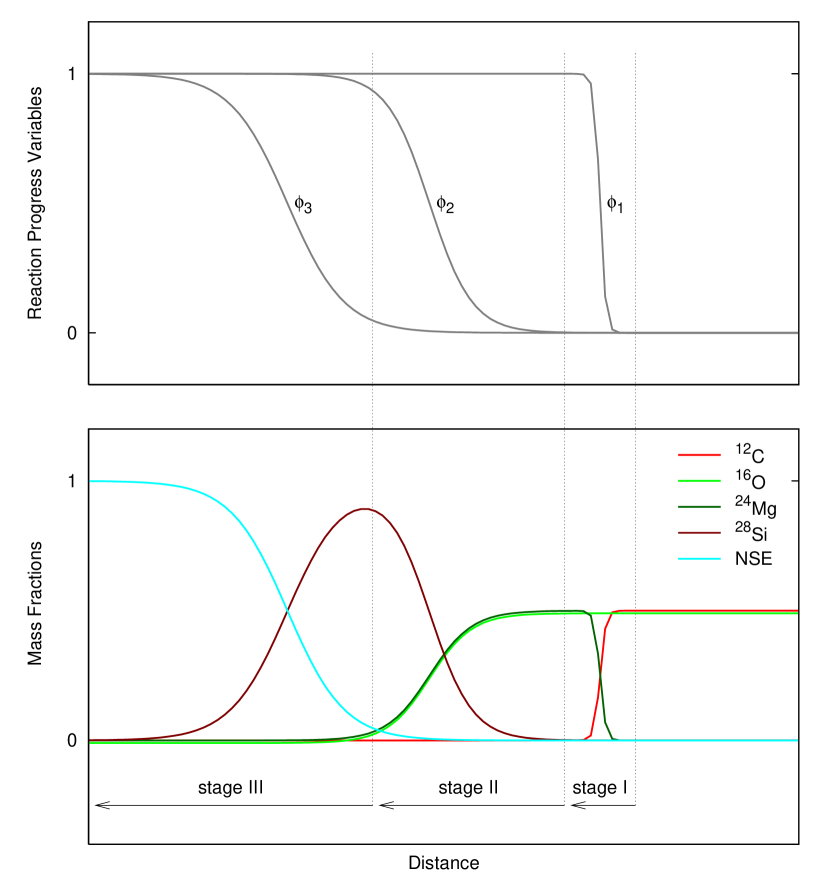
Figure 6.— Diagram of three-stage model flame front structure for a flame propagating to the right. The upper panel shows the progress variables used to track the flame activity: $\phi_{1}$ models the $\mathrm{{}^{12}C}$ flame front, $\phi_{2}$ models progress to NSQE, and $\phi_{3}$ models relaxation to NSE. The lower panel demonstrates the elements used to represent the stages and their relation to the progress variables.

As mentioned in section 2, the structure of the nuclear flame can be modeled as a three-stage process in which each consecutive stage occurs on a longer timescale. In our model, the progress of each of these stages is tracked with progress variables $\phi_{1}$, $\phi_{2}$, and $\phi_{3}$, which evolve from 0 to 1. This is shown schematically in the upper panel of Fig. 6, where the flame is propagating to the right. Material begins as a mixture of $\mathrm{{}^{12}C}$ and $\mathrm{{}^{16}O}$. In stage 1, the $\mathrm{{}^{12}C}$ is consumed, in stage 2, the resulting ash burns to NSQE, and finally in stage 3 material relaxes to actual NSE. The NSQE state is reached much more quickly than the final NSE state, and most ($>90\%$) of the energy release in burning to NSE is released upon reaching NSQE (Khokhlov, 1995). Having separate progress variables for NSQE and NSE allows the energy release timescale to be properly modeled while still tracking when material will reach actual NSE abundances. The resulting NSE state is not static, but can change as the material evolves hydrodynamically (e.g. decompression in a rising bubble), and due to weak interactions. The treatment of this post-flame NSE evolution is described in section 5.

Because the burning of $\mathrm{{}^{12}C}$ occurs on much less than the grid scale, and the physical scale of this flame front is an important factor in setting its propagation speed, the ADR flame scheme is used to evolve $\phi_{1}$ with the parameterized flame speed discussed above. This reflects the propagation of the actual flame front through the star. Although the consecutive stages separate cleanly on a microscopic level, as indicated in figures 2-4, in order to allow for proper advection of the unresolved transition fronts in the model, all three stages are allowed to be partially progressed in the same cell. However, later flame stages only progress when previous flame stages have completed. When $\phi_{1}<1$, $\dot{\phi}_{2}=0$, but behind the propagating $\mathrm{{}^{12}C}$ flame, when $\phi_{1}=1$,

$$\dot{\phi}_{2}=\frac{1-\phi_{2}}{\tau_{\rm NSQE}}.$$ (8)

Here $\tau_{\rm NSQE}$ is the timescale for reaching the NSQE state evaluated in nuclear network studies discussed in detail in the following section. The speed of this evolution and that for $\phi_{3}$ below are limited such that $\phi_{2}$ will change by at most 2% in a single explicit hydrodynamic timestep, in order to reduce noise.

As noted earlier, the bulk of the energy released in the burn to NSE is released upon reaching NSQE. Accordingly, and for simplicity, all the energy available in the initial burn to NSE is released in the first two stages, so that the nuclear energy release in the flame is given by

$$\epsilon_{\rm nuc}=\left\{\begin{array}[]{ll}\dot{\phi}_{1}\Delta Q_{\rm C}+\dot{\phi}_{2}(\Delta Q_{NSE}-\Delta Q_{\rm C})&\text{when$\Delta Q_{\rm NSE } > \Delta Q_{\rm C}$,}\\ \\ \dot{\phi}_{1}\Delta Q_{\rm NSE}&\text{when$\Delta Q_{\rm NSE} < \Delta Q_{\rm C}$.}\\ \end{array}\right.$$ (9)

Here $\Delta Q_{\rm C}$ is the energy release for burning the initial abundance of $\mathrm{{}^{12}C}$ to $\mathrm{{}^{24}Mg}$  and $\Delta Q_{\rm NSE}$ is the energy released for burning to NSE. $\Delta Q_{\rm NSE}$ is a function of the local density, and is evaluated in detail in the next section. Even at high densities, $\Delta Q_{\rm NSE}>3\times 10^{17}\,\mathrm{ergs\,g^{-1}}$ (see Fig. 8). The $\mathrm{{}^{12}C}$ burning releases $\Delta Q_{\rm C}=2.78\times 10^{17}\,\mathrm{ergs\,g^{-1}}$ for $X_{\rm C}=0.5$, and, accordingly, the second form in equation (9) is not used in the simulations presented in this work.

Finally, after NSQE is reached, the final progress variable is evolved. When $\phi_{2}=1$,

$$\dot{\phi}_{3}=\frac{1-\phi_{3}}{\tau_{\rm NSE}},$$ (10)

where $\tau_{\rm NSE}$, evaluated below, is the timescale on which full relaxation to the NSE abundance distribution occurs. The evolution of the NSE state is delayed until the third progress variable reaches unity. Our intention is to allow a clear structure of the flame at low densities where the stages will separate significantly, and where post-flame NSE evolution is expected to be of relatively minor importance. At high densities the NSE timescale is short enough that the post-flame evolution of the NSE state described below in section 5 takes over within a few grid cells of the ADR flame stage ($\phi_{1}$). Note that because $\phi_{2}$ and $\phi_{3}$ are not ADR variables, the flame is not significantly thickened by the addition of multiple burning stages.

By inspecting the evolution shown by the isochoric self-heating calculations in section 2, we find that the abundance evolution can be approximated by selected abundant elements in the intermediate stages. The stages then correspond to the following transitions: stage 1, $\mathrm{{}^{12}C}$ $\rightarrow$ $\mathrm{{}^{24}Mg}$; stage 2, $\mathrm{{}^{24}Mg}$ & $\mathrm{{}^{16}O}$ $\rightarrow$ $\mathrm{{}^{28}Si}$; stage 3, $\mathrm{{}^{28}Si}$ $\rightarrow$ NSE. This allows the abundances to be related to the progress variables, giving

$$X_{{}^{12}\rm C} = (1-\phi_{1})X_{\rm C}^{0},$$ (11)

$$X_{{}^{16}\rm O} = (1-\phi_{2})(1-X_{\rm C}^{0}),$$ (12)

$$X_{{}^{24}\rm Mg} = (\phi_{1}-\phi_{2})X_{\rm C}^{0},$$ (13)

$$X_{{}^{28}\rm Si} = (\phi_{2}-\phi_{3}),$$ (14)

$$\phi_{3} = \sum X_{i,\rm NSE},$$ (15)

where $X_{\rm C}^{0}$ is the initial abundance of $\mathrm{{}^{12}C}$ and the $X_{i,\rm NSE}$ consists of the elements that make up the NSE abundances. The relationship between the progress variables and the abundances, and their evolution, is demonstrated in Fig. 6. The distribution of material among the NSE elements which together make up $\phi_{3}$ is found from

$$\dot{X}_{i}=\dot{\phi}_{3}X_{i,\rm NSE}^{\rm sh}(\rho)$$ (16)

and advecting the results in the usual way. Here the $X_{i,\rm NSE}^{\rm sh}(\rho)$ result from the same self-heating calculation used to find $\Delta Q_{NSE}$, described in the following section. This also provides a reasonable crossover to the post-flame evolution of the NSE element abundances described below. NSE material with approximately the correct density dependent binding energy is monotonically produced by the flame.

4. Input to the Flame model from network and NSE calculations

The three stage model flame front (Fig. 6) requires a priori information characterizing the burn. In this section, we discuss the calibration of the energetics and timescales of the flame model. Using self-heating calculations allows us to make progress by removing the constraint on the size of time steps that occurs with an explicit hydrodynamics method (described above). Our principal approach for determining energetics and timescales is to perform self-heating simulations with the large nuclear reaction network, and this method works for most of the densities of interest. These self-heating calculations must still resolve the temporal evolution of the burn, which for the network calculations is accomplished by employing a variable time step ordinary differential equation integrator. Although requiring small timesteps during some of the evolution, the calculations are tractable. At the lowest densities, however, the relatively long burning timescale forces us to obtain the abundances and binding energy of the NSE state by applying direct NSE calculations to the results of the self-heating network calculations. These calculations are presented in this section, and the direct NSE method is described in Appendix A. As mentioned above, the calibration presented here applies to the case of a 1:1 mass ratio of C and O. The model flame may be applied to any constant mass ratio mixture, but would require the calculations described in this section to be repeated for the particular case (and use of the appropriate input flame speed). The effect would be a different calibration, with longer or shorter timescales and a different energy release.

The network we use contains 200 nuclides up to Kr, shown in Fig. 7. We solve the evolution of the species and heat equation in time,

$$\frac{dY_{i}}{dt} = \frac{1}{\rho N_{\rm A}}(-r_{\rm dest}^{(i)}+r_{\rm prod}^{(i)})\ ,$$ (17)

$$\frac{dE}{dt} = \epsilon_{\rm nucl}+\frac{P}{\rho^{2}}\frac{d\rho}{dt}\ ,$$ (18)

where $Y_{i}$ is the abundance of species $i$ in mol g^-1, and E is the internal energy per gram. The term $r_{\rm dest}^{(i)}(r_{\rm prod}^{(i)})$ is the destruction (production) rate per volume of species $i$ owing to thermonuclear reactions, which is in fact a sum over all the reaction paths in which the nuclide participates. $\epsilon_{\rm nucl}$ is the energy generation rate due to thermonuclear burning, a sum of the reaction $Q$-values for each pathway times their rates per gram of material. We solve for the evolution of the nuclide abundances and heat equation, eq. (17) and eq. (18), using an operator-split formalism. For constant pressure, eq. (18) can be written as

$$\frac{dT}{dt}=\epsilon_{\rm nucl}\cdot\left[C_{\rm V}+\left(\frac{P}{\rho^{2}}-\frac{\partial E}{\partial\rho}\right)\frac{\partial P/\partial T}{\partial P/\partial\rho}\right]^{-1}\ ,$$ (19)

where all partial derivatives are either at constant $T$ or $\rho$, and $C_{\rm V}=\frac{\partial E}{\partial T}$ is specific heat in constant density. In writing eq. (19), we neglect the terms of change in internal energy due to the change in the species. These terms are quite small compared with $\epsilon_{\rm nucl}$ except right at NSE. Eq. (17) is stepped forward in time at a constant $T$ and $\rho$ using a semi-implicit scheme combined with a sparse matrix solver (see Timmes, 1999, and references therein). $T$ is updated by finite differencing (19) and solving explicitly. When $d\rho/dt=0$ (isochoric), eq. (18) is simplified to be $dE/dt=\epsilon_{\rm nucl}$, i.e., all the energy input from nuclear burning is used to increase the internal energy and hence the temperature. In this case, we update $T$ from the updated $E$ via nuclear burning by calling the equation of state, which takes into account the contribution due to the change in the species. For constant $P$ (isobaric), some part of the burning energy is used to expand the material. Using the constant P and updated T (eq. 19), $\rho$ can be updated by calling the equation of state.

The thermonuclear reaction rates are taken from an expanded version  of the rate compilation REACLIB (Thielemann et al., 1986; Rauscher & Thielemann, 2000). We have also included the temperature-dependent nuclear partition functions provided by Rauscher & Thielemann (2000), both in the determination of the rates of inverse reactions and in our determination of NSE abundance patterns. To ensure that the rates obey detailed balance in NSE, the inverse reaction rates are derived directly from the forward rates based upon equilibrium equations that account for Coulomb interactions on the chemical potential (see Appendix A). Our calculations demonstrate that the average binding energy and the abundances of the final NSE state from the self-heating calculation agrees with the results of direct NSE calculations to within $1\%$. We incorporate the effects of electron screening of thermonuclear reaction rates, adopting the relations for weak screening and strong screening provided by Wallace et al. (1982). Finally, contributions from weak reactions are included using the rates provided by Langanke & Martínez-Pinedo (2000, 2001).

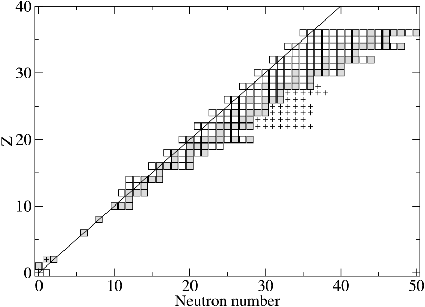
Figure 7.— Set of nuclides included in the 200 nuclide network (boxes) and additional neutron rich nuclides added for the NSE calculations (crosses). Shaded boxes indicate stable nuclides.

We apply this network in a collection of representative self-heating calculations, which are intended to inform our flame model both of the timescales required to reach NSQE or NSE and of the accompanying nuclear energy release. As discussed in § 2, an isochoric calculation provides a good representation of the burning in an actual flame. We also use isochoric calculations below to discuss the importance of screening. The initial temperature is set as $T_{9}=1.7$, which is sufficient for $\mathrm{{}^{12}C}$ and $\mathrm{{}^{16}O}$ ignition but lower than the final temperatures obtained at NSE for the densities of interest. As with all calculations featured in this work, the initial composition was taken to be half $\mathrm{{}^{12}C}$ and half $\mathrm{{}^{16}O}$ by mass. The calculations were continued until NSE was achieved, except at lower densities ($\rho<10^{7}\ \mathrm{g\ cm^{-3}}$), for which the timescales to reach NSE are extremely long. Although the self-heating calculations at very low densities do not yield the correct NSE composition and released energy, they do provide temperatures close to those of the NSE states. Hence, we apply the temperature achieved from the self-heating calculation to the direct NSE calculation to get the correct released energy and composition.

The results of these systematic studies are presented in Table 3 and 4, where, for the critical range of densities, we tabulate the temperature achieved, the energy release in erg/g, and the mass fractions of ⁴He and protons. The results from two other networks, aprox19 and torch47 (Timmes, 1999), are listed as a comparison for the isochoric case. As a reference point, the conversion of an initial composition of half $\mathrm{{}^{12}C}$ and half $\mathrm{{}^{16}O}$ by mass (with a mean binding energy per nucleon of 7.829 MeV/nucleon) to pure $\mathrm{{}^{56}Ni}$ (8.643 MeV/nucleon) yields 0.814 MeV/nucleon or equivalently $7.85\times 10^{17}$ erg/g. The lower values of the energy release contained in Table 3 reflect the presence of significant concentrations of ⁴He (7.074 MeV/nucleon) and protons; these are characteristic of NSE distributions at higher temperatures, and can be seen to increase with increasing density and temperature. Reliable determinations of the compositions under these conditions are clearly crucial to our obtaining a proper measure of the energy release, as described in our discussion of the implementation of our flame energetics.

Figure 8.— Energy released and NSE temperature for burning C/O as functions of density of the fuel for isochoric self-heating calculations with (solid lines) and without (dashed lines) electron screening and Coulomb corrections. For comparison, the contour corresponding to the condition (for $Y_{e}$ = 0.5) that the nuclear statistical equilibrium consists of equal parts by mass of ⁴He and ⁵⁶Ni is shown (dotted line).

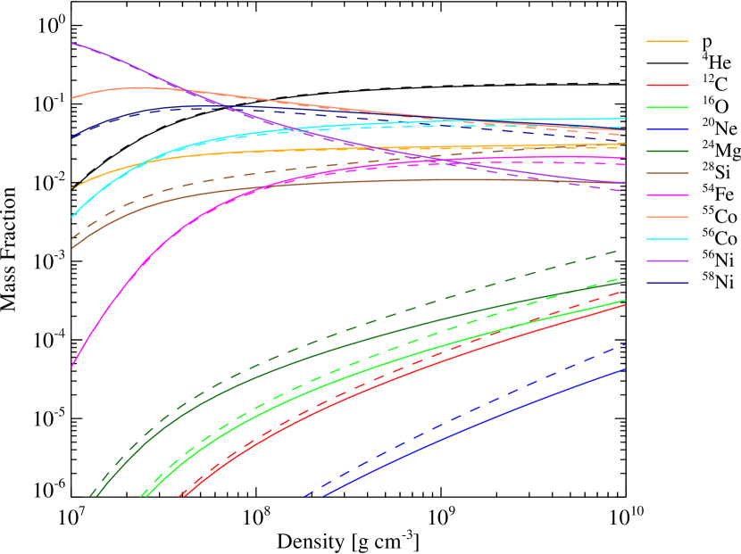
Figure 9.— Final (NSE) abundances of select species after C/O burning for the cases shown in Fig. 8. Dashed and solid lines have the same meaning as there.

The “ignition line", defined as the temperature-density relation of the final NSE state from the self-heating calculations, is presented in Fig. 8. This is shown for the isochoric case in order to facilitate the discussion of Coulomb screening corrections below. At all of the densities shown the electrons are fully degenerate. For comparison, we sketch the contour in the log$\rho-T_{9}$ plane corresponding to the condition (for $Y_{e}$ = 0.5) that the nuclear statistical equilibrium consists of equal parts by mass of ⁴He and ⁵⁶Ni. The greatest proximity of our ignition line to the equal mass ⁴He/⁵⁶Ni contour is seen to occur at the highest densities (e.g. $10^{9}~{}{\rm g\,cm^{-3}}$) and correspondingly high temperatures. The free particle densities realized for the case $\rho$ = 10⁷ are considerably lower, the matter is dominated by iron-peak nuclei, and the corresponding mean binding energy per nucleon most closely approaches that of pure ⁵⁶Ni. Note that our ignition line can approach - but never overlay - the equal mass ⁴He/⁵⁶Ni contour for a very straightforward reason. Recall that our initial condition consisted of equal masses of ¹²C and ¹⁶O; the mean binding energy per nucleon for this mixture is $\sim$ 7.8 MeV/nucleon. However, the mean B/A for a mixture of equal parts by mass ⁴He and ⁵⁶Ni is also B/A$\sim$7.8 MeV/nucleon. It follows that the ⁴He-⁵⁶Ni contour is physically not achievable for this fuel composition.

4.1. Coulomb Correction and Energetics

The impact of our inclusion of Coulomb corrections and screening effects both on the NSE temperatures achieved and on the energetics are illustrated in Fig. 8. A detailed discussion of the manner in which Coulomb and screening effects are utilized in the determination of screened reaction rates and nuclear statistical equilibrium configurations is presented in Appendix A. In order to facilitate comparison, the case without screening neglects both reaction rate screening and Coulomb corrections to the equation of state (EOS). This necessitates an isochoric comparison due to the lower pressure with Coulomb corrections in the EOS. We note from the figure that even at the highest densities, where screening effects are most pronounced ($\Gamma_{{}^{56}\rm Ni}=Z^{5/3}e^{2}(4\pi n_{e}/3)^{1/3}/kT=10$), the differences in energy release is negligible and the differences in temperatures achieved are quite small. For the limiting case of $\rho=10^{10}$ g cm^-3, the temperature achieved without screening and Coulomb correction is $T_{9}=10$ while with screening it is $T_{9}=10.5$, increasing by $5\%$. For the same conditions, the difference in energy release is less than $1\%$.

In order to understand how plasma Coulomb corrections affect the final temperature and energy release, it is useful to look at how the final (NSE) composition changes in detail. Fig. 9 demonstrates the difference of the NSE compositions with screened (solid lines) and unscreened (dashed lines) network calculations. The difference is again quite modest. Generally the inclusion of plasma Coulomb corrections energetically favors assembling fewer, higher charge ions from lower charge ones. Consistent with this, we find that the abundances of the high-charge species increase at the expense of low-charge ones. In light of the minor change in abundances, the ideal-gas contribution to the heat capacity (which is related to the mean molecular weight of the ion gas) changes very little. Thus the the difference in temperature at the high density between the screened and unscreened cases is likely due to the difference in the EOS being used. The Coulomb corrections decrease the heat capacity of the ion gas, allowing higher temperatures to be reached for the same energy release.

The degree of agreement between the energy release with and without screening terms is remarkable. A clue to the origin of this match is that there is one exception to the general rule that Coulomb enhances heavy element abundances: protons. Although the ⁴He, ¹²C, and ¹⁶O abundances are decreased in the screened case, protons actually increase. This is because we are working with the constraint that $Y_{e}=0.5$, while ⁵⁶Ni is by far not the most abundant Fe-group nucleus, with more neutron-rich nuclides like ⁵⁶Co and ⁵⁸Ni being favored. Thus it appears that although high-charge nuclei are favored with screening included, this is offset in energy release by the concomitant increase in proton abundance.

Table 2NSQE and NSE timescales from self-heating network calculations with the 200 nuclide network.

		max. $\mathrm{{}^{28}Si}$ abund.	90% of $\mathrm{{}^{56}Ni}$ abund.	90% of Fe-peak nucleus	90% of NSE nuclei
log($\rho$)	$T_{\rm NSE}$	$\tau_{\rm NSQE}$	$\tau_{\rm NSE}$	$\tau_{\rm NSE}$	$\tau_{\rm NSE}$
($\ \mathrm{g\ cm^{-3}}$)	($10^{9}$ K)	(s)	(s)	(s)	(s)
7.0	4.56	2.21E-03	2.90E+00	2.90E+00	2.86E+00
7.1	4.75	5.46E-04	6.62E-01	6.62E-01	6.65E-01
7.2	4.95	1.39E-04	1.70E-01	1.70E-01	1.68E-01
7.3	5.13	3.75E-05	4.94E-02	4.94E-02	4.56E-02
7.4	5.32	1.07E-05	1.19E-02	1.19E-02	9.40E-03
7.5	5.50	3.28E-06	4.33E-03	7.16E-04	3.02E-03
7.6	5.68	1.08E-06	1.72E-03	2.26E-04	1.02E-03
7.7	5.85	3.81E-07	7.80E-04	8.08E-05	3.85E-04
7.8	6.01	1.45E-07	3.61E-04	3.22E-05	1.46E-04
7.9	6.17	5.85E-08	1.68E-04	1.45E-05	5.64E-05
8.0	6.33	2.50E-08	8.01E-05	7.08E-06	2.27E-05
8.1	6.50	1.12E-08	3.87E-05	3.66E-06	9.56E-06
8.2	6.66	5.19E-09	1.89E-05	1.97E-06	4.22E-06
8.3	6.82	2.50E-09	9.41E-06	1.10E-06	1.94E-06
8.4	6.99	1.26E-09	4.77E-06	6.01E-07	9.35E-07
8.5	7.15	6.58E-10	2.48E-06	3.45E-07	4.67E-07
8.6	7.33	3.58E-10	1.30E-06	2.03E-07	2.41E-07
8.7	7.50	2.02E-10	7.00E-07	1.20E-07	1.28E-07
8.8	7.68	1.19E-10	3.82E-07	7.17E-08	7.01E-08
8.9	7.87	7.13E-11	2.12E-07	4.32E-08	3.91E-08
9.0	8.06	4.42E-11	1.21E-07	2.52E-08	2.24E-08
9.1	8.26	2.80E-11	6.86E-08	1.55E-08	1.30E-08
9.2	8.47	1.81E-11	3.97E-08	9.50E-09	7.64E-09
9.3	8.69	1.19E-11	2.32E-08	5.88E-09	4.58E-09
9.4	8.92	7.86E-12	1.37E-08	3.61E-09	2.78E-09
9.5	9.16	5.24E-12	8.22E-09	2.23E-09	1.71E-09
9.6	9.40	3.51E-12	4.98E-09	1.41E-09	1.07E-09
9.7	9.60	2.38E-12	3.07E-09	8.98E-10	6.78E-10
9.8	9.94	1.62E-12	1.91E-09	5.90E-10	4.32E-10
9.9	10.2	1.10E-12	1.19E-09	3.86E-10	2.78E-10
10.0	10.5	7.45E-13	7.66E-10	2.49E-10	1.81E-10

Note. — The NSQE timescale is defined as the elapsed time in a simulation between the point at which 90% of the C has burned to the maximum of $\mathrm{{}^{28}Si}$ abundance. The time scales to NSE were determined as the elapsed time from the maximum abundance of ²⁸Si, to the 90% of the maximum ⁵⁶Ni abundance, to the 90% of the maximum abundance of the most abundant Fe-peak nucleus, and to 90% of the maximum number of NSE nuclei, respectively. NSE nuclei were ⁴He and isotopes of Cr, Fe, Co, Ni, and Zn.

4.2. NSQE and NSE timescale calculations

Figure 10.— Nuclear burning timescales versus ash temperature of C/O fuel calculated by 200 nuclide self-heating network. Shown are curves for the timescales to NSQE and NSE for isochoric (solid lines) and for isobaric (dashed lines) one-zone calculations.

Figure 11.— Nuclear burning timescales versus density of C/O fuel calculated by 200 nuclide self-heating network. Shown are curves for the timescales to reach NSQE and NSE with (solid lines) or without (dashed lines) screening and Coulomb corrections for an isochoric burn and with corrections for an isobaric burn (dash-dot lines). Superposed is the dynamical timescale (dotted line), $\tau_{\rm dyn}$.

As noted above, the three-stage flame model requires timescales for the second and third stages of burning. These timescales must be determined in advance of simulations with the three-stage flame model, and accordingly we investigated determining these timescales with the self-heating networks available to us, and the effect of screening on these timescales.

The timescale to NSQE was defined as the elapsed time in a simulation between the point at which 90% of the C has burned and the maximum abundance of ²⁸Si. Defining the timescale to NSE requires a little more care, and we investigated several approaches. In all cases, the timescale was measured as the elapsed time from the maximum abundance of ²⁸Si. The results of these studies are shown in Table 2. In Table 2 we list the NSE timescales defined in several ways: the time when 90% of the maximum $\mathrm{{}^{56}Ni}$ abundance is reached; the time when 90% of the maximum abundance of the most abundant Fe-peak isotope is reached; the time when 90% of the maximum abundance of NSE nuclei is reached. NSE nuclei include $\mathrm{{}^{4}He}$ and isotopes of Cr, Fe, Co, Ni, and Zn. At the lowest density end, Ni dominates the NSE compositions, so all the approaches yield the same NSE timescales. At the highest density end, the dominant NSE composition is a mixture of He and Fe-peak isotopes. By including Fe-peak nuclides other than Ni, we can see that the timescales differ at most within a factor of 3 at the high density end. Including He decreases the timescale further by a factor of 1.5 at the high density end. In this paper, we choose the last definition as NSE timescale in implementing the flame model. The NSQE and NSE timescales from the self-heating calculations are fitted by

$$\tau_{\rm NSQE}=\exp{(182.06/T_{9}-46.054)}$$ (20)

and

$$\tau_{\rm NSE}=\exp{(196.02/T_{9}-41.645)}\ .$$ (21)

We express the timescales as functions of final temperature, which is determined by the final density and energy release in self-heating calculations. This is a quite robust parameterization as seen from the comparison of timescales determined from isochoric and isobaric calculations in Fig. 10. We note that our NSQE/NSE timescales are consistently lower than those of Khokhlov (1991a), but we are unable to determine the reason for this difference.

The influence of screening on the burning timescales, as inferred from our self-heating calculations, is revealed in Fig. 11. Once again we use an isochoric case to isolate the effects of rate screening. In contrast to our findings for temperature and energy, the impact of the inclusion of Coulomb and screening effects is seen here to decrease the timescales to achieve NSQE and NSE by factors of 2–3. This reflects the level of individual screening enhancements for the critical reactions that govern the flows into the iron-peak region. An isobaric burn, representative of what will occur in the star, is also shown, and has much longer timescales at lower densities due to the lower temperature on expansion. For comparison, the dynamical timescale for homologous collapse, $\tau_{\rm dyn}=(24\pi G\rho)^{-1/2}=0.14(10^{7}\;\ \mathrm{g\ cm^{-3}}/\rho)^{1/2}~{}{\rm s}$, is superposed (dotted line) on the figure. Note that $\tau_{\mathrm{NSE}}>\tau_{\mathrm{dyn}}$ for $\rho<4\times 10^{7}\;\ \mathrm{g\ cm^{-3}}$ and $\tau_{\mathrm{NSQE}}>\tau_{\mathrm{dyn}}$ for $\rho<1.5\times 10^{7}\;\ \mathrm{g\ cm^{-3}}$.

5. Post-flame energy release and neutronization

Once the flame has passed through a piece of stellar material, the remaining ashes have burned to NSE, which is predominantly comprised of iron-peak nuclei, ⁴He, and free protons. This NSE composition, however, should not be considered static. It changes as the density decreases, either in a rising bubble or due to the expansion of the star, resulting in a varying ionic heat capacity and more importantly causing the difference in nuclear binding energy between the initial $\mathrm{{}^{12}C}$/$\mathrm{{}^{16}O}$ fuel and the NSE state to vary during the course of the hydrodynamic evolution of the supernova. During this extended evolution, there is time for weak interactions to take place in the ash material. Dominated by electron captures, these processes lower $Y_{e}$ and emit neutrinos. Below we discuss these two physically distinct effects which bring about changes in the NSE abundances. The method used to calculate (Coulomb-corrected) NSE is described in Appendix A, with the set of nuclides used in our network calculation supplemented with neutron-rich Fe peak elements as shown in Fig. 7.

5.1. NSE adjustment to the evolving state variables $\rho$ and T

The hydrodynamic evolution of the ashes, i.e. the expansion following the burn, causes a decrease in $\rho$ and $T$ on a hydrodynamic timescale, which in turn causes a change in the NSE mass fractions as the nucleons reorganize to maximize entropy for the new thermodynamic state. As long as the hydrodynamic timescale substantially exceeds the charged-particle (strong) nuclear reaction timescale, the approximation of instantaneous readjustment of the composition of the ashes to the NSE appropriate for the local thermodynamic state is a good one.

Figure 12.— Contours of binding energy per nucleon, $q$, in MeV per nucleon, for the NSE state with $Y_{e}=0.5$. Also shown is as a function of density the final temperature reached (dot-dashed line) by the 200 nuclide self-heating network calculation starting from an equal mixture of C and O by mass and burning to NSE. The line of 50% $\mathrm{{}^{56}Ni}$ mass fraction (dotted line) in a two-component NSE ($\mathrm{{}^{4}He}$ and $\mathrm{{}^{56}Ni}$) indicates the temperature above which light particles dominate.

The electron fraction, defined as $Y_{e}=\sum_{i}{Z_{i}\frac{X_{i}}{m_{i}}}/\sum_{i}{A_{i}\frac{X_{i}}{m_{i}}}$, where $m_{i}$ is the nuclear mass of species $i$, of the $\mathrm{{}^{12}C}$/$\mathrm{{}^{16}O}$ mixture is 0.5. Weak interactions are assumed to be negligible during the burning phase of the flame since the weak interaction timescale far exceeds the burning timescale. At first, the composition of the hot, unexpanded ashes has a significant fraction of the mass in free protons (0 MeV) and $\mathrm{{}^{4}He}$ (7.074 MeV/nucleon). For example at $\rho_{8}=1,\mathrm{X}_{\mathrm{p}}=0.024,\mathrm{X}_{\mathrm{He}}=0.095$ and at $\rho_{8}=10,\mathrm{X}_{\mathrm{p}}=0.027,\mathrm{X}_{\mathrm{He}}=0.135$. The remainder predominantly consists of a mix of strongly bound Fe-peak nuclei, dominated by $\mathrm{{}^{54}Fe}$. The nuclear binding energies reached in the hot ashes immediately following the burn are therefore significantly smaller than the binding energies obtained by a cold NSE dominated by $\mathrm{{}^{56}Ni}$  and lie along the dot-dashed line in Fig. 12.

The binding energy gain per nucleon of such a mixture compared to the initial $\mathrm{{}^{12}C}$/$\mathrm{{}^{16}O}$ fuel, which has a binding energy per nucleon of 7.828 MeV, varies with density but remains for $\rho_{8}>1$ in the vicinity of 0.4 MeV. As the material expands and cools, NSE progressively favors heavier nuclei. The reason for the shift from an alpha rich NSE to an alpha poor NSE during an expansion is that lower entropies allow for a reduction of the total number of particles, since the number of accessible microstates of the ensemble has decreased. The light particles are reassembled into fewer but more tightly bound Fe-peak nuclei. At constant $Y_{e}=0.5$, the composition would reach virtually 100% $\mathrm{{}^{56}Ni}$ at freezeout temperatures. In other words, at constant $Y_{e}=0.5$, the binding energy would shift from $\sim$ 8.2 to 8.643 MeV per nucleon and an additional $\sim$ 0.4 MeV of binding energy would be released per nucleon during the expansion phase. This is a significant fraction of the total energy released and must be accounted for.

Furthermore, because the average nucleon number per nucleus $\bar{A}=\sum_{i}{A_{i}\frac{X_{i}}{m_{i}}}/\sum_{i}{\frac{X_{i}}{m_{i}}}$ grows as the NSE distribution is further shifted with decreasing temperature toward the iron-peak nuclei, the ionic heat capacity decreases. Because we have conditions that are at the borderline of electron degeneracy, we estimate this to have a small effect.

5.2. Neutronization

Virtually all extant one-dimensional calculations of SNe Ia explosions find that the innermost regions (the inner $\approx$ 0.2 M_⊙) suffer sufficient changes in $Y_{e}$, due to electron captures, to significantly change the compositions (Nomoto et al., 1984; Khokhlov, 1991b; Iwamoto et al., 1999). The use of recent electron capture rates, based on shell model diagonalization, reduces the neutron excess in the central regions somewhat (Brachwitz et al., 2000), the gross features however remain. Neutronization is a consequence of the high Fermi energies and the correspondingly high rates of electron capture reactions under these conditions. The time rate of change of the electron fraction $\dot{Y_{e}}$, also referred to as the neutronization rate, and the amount of energy carried away by neutrinos per gram of stellar material per second $\dot{E^{\nu}}$ are calculated as NSE averages by convolving tabulated weak interaction rates (Langanke & Martínez-Pinedo, 2001) with the NSE abundances. We consider electron decay, positron captures, electron captures and positron decay of pf-Shell nuclei as well as free nucleons, so that

$$\dot{Y_{e}} = \sum_{i}{\frac{X_{i}m_{u}}{m_{i}}\Big{(}\lambda^{ed}_{i}+\lambda^{pc}_{i}-\lambda^{ec}_{i}-\lambda^{pd}_{i}\Big{)}}$$ (22)

$$\dot{E^{\nu}} = \sum_{i}{\frac{X_{i}m_{u}}{m_{i}}\Big{(}\lambda^{\bar{\nu}}_{i}+\lambda^{\nu}_{i}\Big{)}}$$ (23)

where we are following the notation from Langanke & Martínez-Pinedo (2001) in which $\lambda^{ed},\lambda^{pc},\lambda^{ec},\lambda^{pd}$ are given in units of $\mathrm{s}^{-1}$ and $\lambda^{\bar{\nu}},\lambda^{\nu}$ are given in units of $\mathrm{MeV}\;\mathrm{s}^{-1}$. Neutrinos emitted are taken to be free-streaming.

At high densities ($\rho_{9}\gtrsim 1$) the NSE averaged neutronization rate for self conjugate matter is rather fast with $-0.05\ {\rm s^{-1}}\gtrsim\dot{Y}_{e}\gtrsim-0.5\ {\rm s^{-1}}$ (see Fig. 13). The rate of neutronization is strongly dependent on the electron fraction (compare Figs. 13 and 14), since electron capture rates are overall decreasing with increasing neutron number for a given element. Due to the strong decrease of the rate of neutronization with decreasing electron fraction, one typically finds the composition of these inner regions to consist of moderately neutron-rich, strongly bound iron-peak nuclei, viz; ⁵⁶Fe, ⁵⁴Fe, and ⁵⁸Ni.

Figure 13.— Contours of time derivative of electron fraction, $\dot{Y}_{e}$, due to electron and positron capture and emission, evaluated at $Y_{e}=0.5$. Other lines are as in Fig. 12.

Figure 14.— Contours of time derivative of electron fraction, $\dot{Y}_{e}$, due to electron and positron capture and emission, evaluated at $Y_{e}=0.48$. Other lines are as in Fig. 12.

If neutronization occurs rapidly enough to lower $Y_{e}$ to $\sim 0.48$, then the binding energy per nucleon of the neutron rich NSE state compared to the NSE state with $Y_{e}=0.5$ is increased by $\sim(0.2-0.3)$ MeV for a range of given temperatures and densities (compare Figs. 12 and 15). In the cold NSE limit, where ⁵⁴Fe (8.736 MeV/nucleon) and ⁵⁸Ni (8.732 MeV/nucleon) are the dominant nuclei of the $Y_{e}=0.48$ NSE abundance distribution, the final binding energy per nucleon increase compared to NSE of self conjugate matter, which is entirely dominated by ⁵⁶Ni, is on the order of 0.14 MeV. Not all of this energy, however, remains available to expand the star. Neutrino losses accompanying neutronization impact the energetics: some fraction of the energy release (being somewhat dependent upon the density and corresponding electron Fermi energy) will be lost in neutrinos (see Figs. 16 & 17).

Figure 15.— Contours of binding energy per nucleon, $q$, in MeV per nucleon, for the NSE state with $Y_{e}=0.48$. Other lines are as in Fig. 12.

Figure 16.— Contours of neutrino energy loss rates, $\epsilon_{\nu}$, during electron and positron captures and emissions, evaluated at $Y_{e}=0.5$. Other lines are as in Fig. 12

.

Figure 17.— Contours of neutrino energy loss rates, $\epsilon_{\nu}$, during electron and positron captures and emissions, evaluated at $Y_{e}=0.48$. Other lines are as in Fig. 12

.

Another important effect of neutronization lies in its effect on the Fermi level of the electrons. As electrons get captured, $Y_{e}$ decreases and since relativistic electron degeneracy pressure scales as $(\rho Y_{e})^{\frac{4}{3}}$ this results in a change in the ratio of electron degeneracy pressure to ionic pressure. Because we are close to the borderline of degeneracy, it is difficult to estimate the impact of this effect on the thermal histories of tracer particles being followed in the simulation.

The impact of neutronization on the rise times of hot bubbles and the subsequent growth of the Rayleigh Taylor instabilities could help to distinguish between competing ignition scenarios. In addition, it affects the relation between the composition of the progenitor white dwarf and the mass of $\mathrm{{}^{56}Ni}$ synthesized in the explosion (Timmes et al., 2003).

5.3. Reduced Set of Nuclei for Evolution in NSE

While the NSE state is calculated using many nuclear species, it is not feasible to store the abundance of each of these at every grid point. In reality only a small number of quantities which are derivable from the set of abundances, $\{X_{i}\}$, are essential to accurate hydrodynamic and energetic simulation of the NSE material. These are the electron fraction, $Y_{e}$, the average number of nucleons per ion, $\bar{A}$, the average binding energy per nucleon, $\bar{q}=\bar{Q}/\bar{A}$, and the coulomb coupling parameter $\Gamma=\overline{Z^{5/3}}e^{2}(4\pi n_{e}/3)^{1/3}/kT$, where $n_{e}$ is the electron number density. The quantities $Y_{e}$, $\bar{A}$, and $\Gamma$ are required to determine the local pressure from density and internal energy content, while $\bar{q}$ provides a measure of the energy stored as rest mass energy of (comparatively less bound) light nuclei, which is released as the NSE state evolves.

Working in the approximation that $m_{i}=A_{i}$ a.m.u. reduces several quantities to simple sums over the abundance set, $Y_{e}=\sum_{i}X_{i}Z_{i}/A_{i}$, $1/\bar{A}=\sum_{i}X_{i}/A_{i}$, and $\bar{q}=\sum_{i}X_{i}Q_{i}/A_{i}$. This approximation is accurate at the level of $10^{-4}$ for these averages, but is unsatisfactory for the actual calculation of NSE due to its dependence on small relative differences between species. With this simple linear form, we see that it is possible to select a set of abundances $\{X^{\prime}_{i}\}$ which give the same $Y_{e}$, $\bar{A}$ and $\bar{q}$, and give the correct mixing evolution of these quantities (essential for an Eulerian code), but which consists of only a select few elements. This representative set can then be used in the simulation without losing information about the energetic evolution of the material, giving appropriate Lagrangian temperature histories which can be used for post-processing.

Choosing this reduced set is much like finding basis vectors which span the 3D space $(Y_{e},1/\bar{A},q)$, except that $\sum X^{\prime}_{i}$ is constrained to be 1, so that the set must both span and bound the available space. We restrict ourselves to elements which exist in nature and thus have known $(Z/A,1/A,Q/A)$. The goal of this method is to utilize existing hydrodynamic tools which are known to treat the $X_{i}$ properly. An alternative is for the basic quantities $(Y_{e},1/\bar{A},q)$ to be treated directly by the hydrodynamics method, as is done by Khokhlov (1995).

The quantities $Y_{e}$, $\bar{A}$, and $\bar{q}$ are three of the four quantities tracked by the nuclear kinetic equations of Khokhlov (1995) (and related references). The fourth is a variable to track the relaxation from NSQE to NSE, which they approximate to have no effect on the energy release, and which corresponds to our third flame stage. Khokhlov (2000) makes the additional approximation that $\bar{A}$ (their $Y_{\rm i}$) is constant in the ashes.

We do not treat $\Gamma$ in any special way. It is expected, however, that because the representative nuclei do not have very different $Z$ from the real ones, the error is not too bad. NSE is generally a mixture of ⁴He and many species near ⁵⁶Ni, making $\Gamma$ fairly well matched if all the other quantities are matched. Thus the benefit of developing a 4D matching method that includes $\overline{Z^{5/3}}$ does not appear necessary for the Ia supernova problem, where $\Gamma$ is moderate ($\simeq 0.5$), and declining, during the evolution. The simple dependence on a $\Gamma$ which contains $\overline{Z^{5/3}}$ is also not a general feature of Coulomb corrections, but only of a particular approximation used for EOS corrections.

Figure 18.— Binding energy per nucleon $Q/A$ vs. $Z/A$ (respectively $\bar{q}$ and $Y_{e}$ of a pure sample) for nuclei used in simulations. Shown are the 200 nuclei in the dynamic network calculation ($+$), and those that were added to extend the $Y_{e}$ range of the NSE calculation ($\times$). Dashed lines extend toward neutrons on the left and ¹H on the right; ³He is also off the plot. Boxes indicate those included in the representative set. The set of heavy nuclei is chosen to allow spanning of the entire possible area of $q$ and $Y_{e}$ (outlined) and also allows accurate representation of $\bar{A}$, precise matching of $\bar{A}$ is achieved in most cases in all but the lowest $Y_{e}$ portion of the solid-outlined area.

The set of elements we have chosen, which includes several necessary for evolution of the flame, consists of neutrons, ¹H, ⁴He, ²²Ne, ²⁴Mg, ⁵⁶Ni, ⁵⁸Ni, ⁵⁶Fe, ⁶²Ni, ⁶⁴Ni, and ⁸⁶Kr. (The full set in the simulation also includes ¹²C, ¹⁶O, and ²⁸Si, used in the burning stages.) These are shown in Fig. 18 along with the full set used in the nuclear network and NSE calculation. The set of neutron-rich heavy elements is used to follow in detail the energy release as the material neutronizes. At most four species are used to construct a given $(Y_{e},1/\bar{A},\bar{q})$, where the species are chosen by comparing these coordinates to the face planes of the four-sided polyhedra formed by four-element sets, starting from (⁴He, ²⁴Mg, ⁵⁶Ni, ⁵⁸Ni) and walking to more neutron rich elements as necessary. If the desired combination lies outside of polyhedra available with these elements, $\bar{A}$ is not matched and the three species which form the triangle enclosing the $Y_{e}$ and $\bar{q}$ of the state are used. The set above allows us to match $Y_{e}$ and $\bar{q}$ exactly to that of the NSE state for $Y_{e}>0.42$. $\bar{A}$ is also matched exactly in most cases, except for $Y_{e}$ near 0.42, where it may vary from the NSE value by up to 10%.

5.4. Energy Evolution in NSE

The NSE properties of the material are used to evolve the mass-specific thermal energy $\mathcal{E}$, much like a nuclear network would evolve the abundances and $\mathcal{E}$ between hydrodynamic steps. The resulting changes are either driven by the hydrodynamic motion, and thus occur on the same timescale, or are due to neutronization, which occurs on a slow timescale compared to the hydrodynamics. After a hydrodynamic step, the values of $\mathcal{E}_{n}$, $\rho$, $T_{n}$ and $\{X^{\prime}_{i}\}_{n}$ are available at each grid point ($n$ labels the timestep). The $q_{n}$ and $Y_{e,n}$ are calculated from $\{X^{\prime}_{i}\}_{n}$, accounting for how mixing changes these quantities. This state is slightly out of NSE as a consequence of the hydrodynamic evolution and a time interval $\Delta t$ has passed during which some neutronization and neutrino loss has occurred. We calculate $\dot{Y}_{e}$ and $\epsilon_{\nu}$ from tables using $\rho_{n}$, $T_{n}$, and $Y_{e,n}$, and then set $Y_{e,n+1}=Y_{e,n}+\dot{Y}_{e}\Delta t$. These functions are not expected to vary steeply in these variables compared to the amount they will change in a single hydrodynamical step. We then find $T_{n+1}$ by solving

$$\mathcal{E}[T_{n+1},Y_{e,n+1},\bar{A}(T_{n+1},Y_{e,n+1})] - q(T_{n+1},Y_{e,n+1})=$$

$$\mathcal{E}_{n}-q_{n}+\Delta t[-\dot{Y}_{e}N_{A}( m_{e} -m_{n}+m_{p})c^{2}-\epsilon_{\nu}],$$ (24)

at fixed $\rho$. Both $\bar{A}$ and $q$ are tabulated from the NSE calculation using our full set of nuclear species. Finally this temperature is used to calculate $\mathcal{E}_{n+1}$, $q_{n+1}$ and $\bar{A}_{n+1}$, and the procedure described above is used to convert $Y_{e,n+1}$, $\bar{A}_{n+1}$, and $q_{n+1}$ to $\{X^{\prime}_{i}\}_{n+1}$.

6. One-dimensional Flame Model Results

In order to exercise the energy deposition and neutronization methods described, we performed a series of one-dimensional model flame simulations at a variety of densities. In each of these a flame was propagated from left to right through fuel consisting of equal parts by mass of $\mathrm{{}^{12}C}$ and $\mathrm{{}^{16}O}$. In these simulations the input flame speeds were laminar flame speeds (eq. [5]); turbulent flame speeds (eq. [4]) were not used. A reflecting boundary condition was used on the left, where the flame is ignited, and outflow on the right, so that fuel is free to move off the grid as the volume of (less dense) ash increases. A flame is started by setting $\phi_{1}=1$ in a small region (with a smoothed edge) adjacent to the left reflecting boundary and depositing the appropriate energy locally. The Figs. 19–22 show profiles of the abundances for some of the surrogate nuclei and $Y_{e}$ at a time when the flame has propagated most of the way across the domain. Right panels show a detail of the model flame region, which by definition is only several computational zones wide.

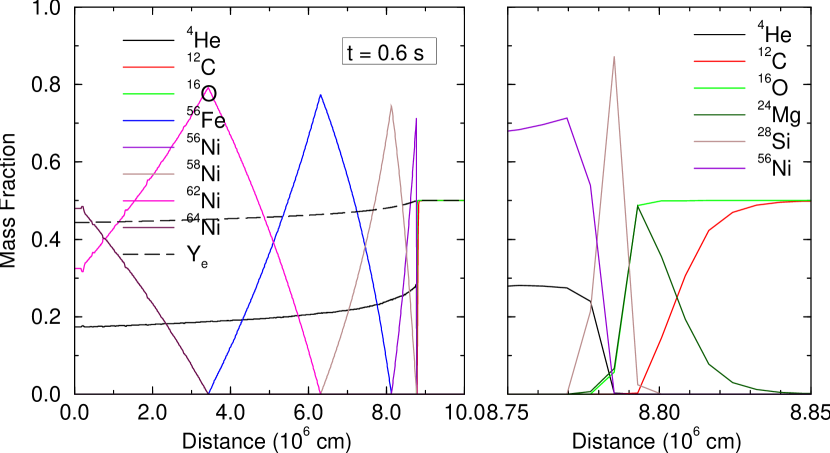
Figure 19.— Abundances from a simulation of a model flame passing through a 50%/50% by mass mixture of C and O at an initial density of $3\times 10^{9}\ \mathrm{g\ cm^{-3}}$. The left panel presents the abundances of selected surrogate nuclei on the entire simulation domain at $t=0.6\mathrm{s}$. Also shown in the left panel is the electron fraction. The right panel shows the detail of the thick flame with another set of surrogate nuclei.

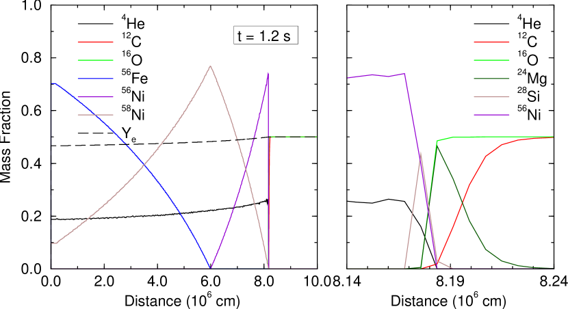
Figure 20.— Abundances from a simulation of a model flame passing through a 50%/50% by mass mixture of C and O at an initial density of $10^{9}\ \mathrm{g\ cm^{-3}}$. The left panel presents the abundances of selected surrogate nuclei on the entire simulation domain at $t=1.2\mathrm{s}$. Also shown in the left panel is the electron fraction. The right panel shows the detail of the thick flame with another set of surrogate nuclei.

Fig.s 19–21 shows the results of a model flames propagating across a $10^{7}\mathrm{cm}$ domain with fuel at densities of $3\times 10^{9}$, $10^{9}$, and $10^{8}\ \mathrm{g\ cm^{-3}}$, respectively. The elapsed times of the simulations are $t=0.6$, $1.2$ and $6.0\ \mathrm{s}$, respectively, and the simulations were performed on a uniform mesh of 1280 points. The material furthest to the left has been burned for the longest time, and therefore has undergone the most neutronization. Moving to the right, ash is younger closer to the propagating flame. The surrogate nuclear set works as expected, with $\mathrm{{}^{4}He}$ and consecutively more neutron rich Fe-peak elements representing the NSE state. The detailed flame structure is also as expected, with the $\mathrm{{}^{12}C}$ burning being followed very closely (within a few zones) by conversion to $\mathrm{{}^{28}Si}$ representing NSQE and that on to NSE. The density dependence of the weak reactions is quite evident. At $3\times 10^{9}\ \mathrm{g\ cm^{-3}}$, $Y_{e}=0.44$ is reached in only 0.6 s, though at $10^{9}\ \mathrm{g\ cm^{-3}}$, even after 1.2 s $Y_{e}$ has only fallen to about 0.47. We performed an additional check on the neutronization by running a self-heating calculation using the 200 nuclide network with weak reactions. Comparing the degree of neutronization, $0.5-Y_{e}$, we found that the self-heating calculation at $10^{9}\ \mathrm{g\ cm^{-3}}$ differed from the leftmost zone of a flame model simulation at initial density of $1.2\times 10^{9}\ \mathrm{g\ cm^{-3}}$ (resulting in an ash density of $10^{9}\ \mathrm{g\ cm^{-3}}$) by 2.6% and 0.7% at 0.6 and 1.2 s respectively. Finally, the speed of the flame in the computational cell due to the creation of the expanded ash is related to the laminar flame speed by $v=S_{\rm laminar}\rho_{\rm fuel}/\rho_{\rm ash}$, and the test simulations reproduce this behavior satisfactorily.

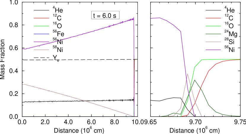
Figure 21.— Abundances from a simulation of a model flame passing through an equal mass mixture of C and O at an initial density of $1.0\times 10^{8}\ \mathrm{g\ cm^{-3}}$. The left panel presents the abundances of selected surrogate nuclei on the entire simulation domain at $t=6.0\mathrm{s}$ Also shown in the left panel is the electron fraction. The right panel shows the detail of the thick flame with another set of surrogate nuclei.

Fig. 22 shows the result of a model flame propagating across a larger $8\times 10^{7}\mathrm{cm}$ domain with fuel at a density of $5.0\times 10^{7}\ \mathrm{g\ cm^{-3}}$. As with the high density simulations, the simulation was performed on a uniform mesh of 1280 points. The slower neutronization time scales with respect to burning necessitated using the larger simulation domain to allow evolution of the flame for a longer time, 16.0 s. In this case, the neutronization following the flame is similar to the higher density flames although the process of neutronization is much slower. The detail of the flame in this case shows a broader $\mathrm{{}^{28}Si}$ region, covering more than six computational zones, indicating that at this low density the flame model is beginning to resolve the NSE timescale.

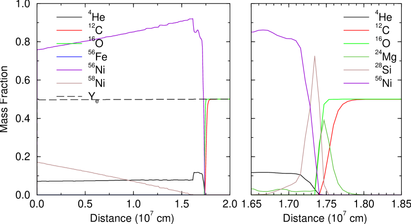
Figure 22.— Abundances from a simulation of a model flame passing through an equal mass mixture of C and O at an initial density of $5.0\times 10^{7}\ \mathrm{g\ cm^{-3}}$. The left panel presents the abundances of selected surrogate nuclei on the entire simulation domain at $t=16.0\mathrm{s}$ Also shown in the left panel is the electron fraction. The right panel shows the detail of the thick flame with another set of surrogate nuclei.

In addition to these results, we performed a variety of test simulations including model flames propagating away from an isolated ignition point in the middle of the domain. A similar calculation in which the fuel was moving at a constant speed across the domain gave identical abundance profiles. The results of these tests are shown in Figs. 23 and 24. In both cases, the high degree of symmetry indicates that the direction in which the flame propagates from the ignition point does not affect the solution. The simulation presented in Fig. 24 tested the ability of the code to correctly propagate the flame in both directions as fuel moves across the grid and indicates a satisfactory result.

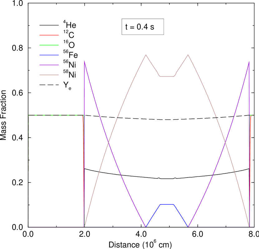
Figure 23.— Abundances and electron fraction from a simulation of a model flame passing through an equal mass mixture of C and O at an initial density of $1.0\times 10^{9}\ \mathrm{g\ cm^{-3}}$. In this case, the “match head" was placed at the center of the domain so that the flame propagated to the left and right. The results may be compared to those of Fig. 20, and the obvious symmetry indicates the flame is correctly propagating in both directions.

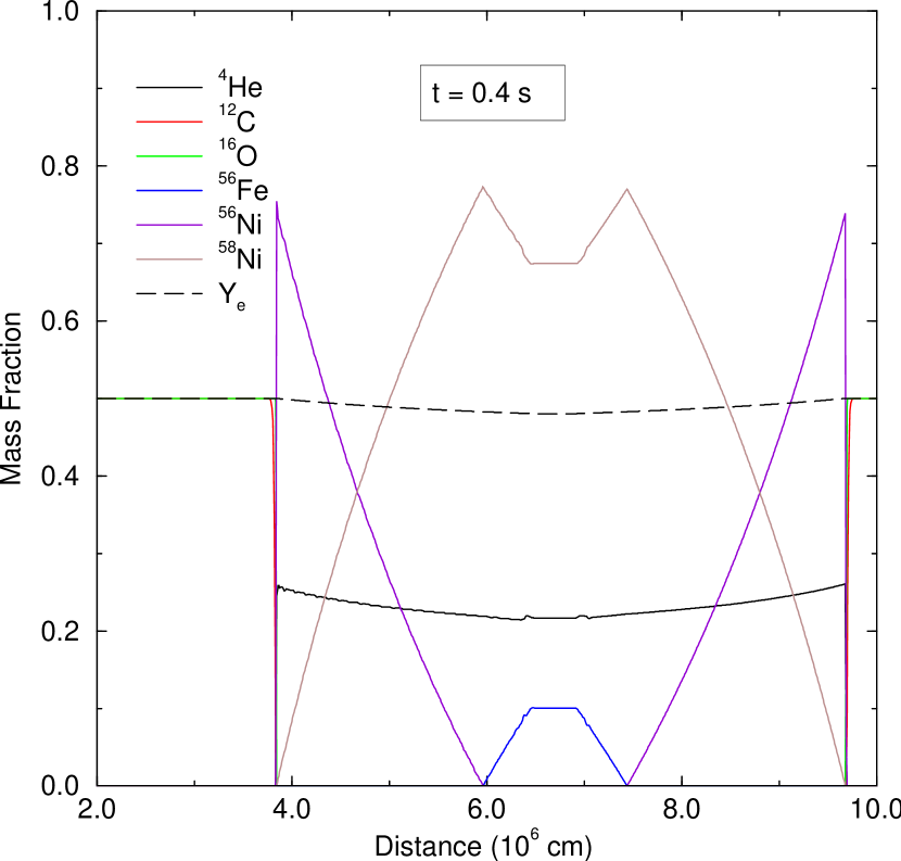
Figure 24.— Abundances and electron fraction from a simulation of a model flame passing through an equal mass mixture of C and O at an initial density of $1.0\times 10^{9}\ \mathrm{g\ cm^{-3}}$. In this case, the “match head" was placed at the center of the domain so that the flame propagated to the left and right while the material on the grid slowly flowed to the right. The results may be compared to those of Fig. 23, the principal difference being that the symmetry is centered about $x=6.6\times 10^{6}$ cm. The obvious symmetry indicates the flame is correctly propagating in both directions and that the slow propagation of the material across the simulation grid does not affect the results.

7. Conclusions

We have extended the ADR flame model (Vladimirova et al., 2006) with multiple burning stages and a reactive NSE post-flame state appropriate for simulations of C/O deflagrations. New calculations were performed to calibrate flame structure, progress timescales, NSE properties and neutronization. This calibration involved detailed calculations of several types, including direct flame simulation with a small nuclear network, one-zone isochoric self-heating nuclear network calculations, and direct NSE calculations. We have described in detail how these calculation justify a parameterized flame model, and what features and timescales must be reproduced in a large-scale simulation. By including Coulomb equation of state corrections to detailed balance, we established self-consistency between screened reaction network calculations and direct NSE calculations. Our neutronization is calculated with up-to-date weak rates (Langanke & Martínez-Pinedo, 2001) convolved with our full NSE distribution. We also developed a method of representing the precise binding energy and $Y_{e}$ of the NSE state with a small set of nuclei that can then be easily treated in a general multi-fluid code.

These improvements are necessary for several reasons. First, full-star models with embedded tracers for nucleosynthetic post-processing are now feasible. Following the passage of the flame, the NSE state evolves as large-scale fluid motions change its temperature and density. At higher densities, electron captures make the NSE state more neutron-rich and lower the pressure from degenerate electrons. Modeling both of these effects is critical for the tracers to capture a high-fidelity recording of the temperature-density history of the burn for subsequent nucleosynthesis calculations. Having a description of the NSE state that follows the post-explosion expansion and freeze-out is also important for evolving models far enough to compute lightcurves for contact with observations.

A second motivation for improving the flame model is to enable simulations of high-central density ignitions. Under these conditions, electron captures can play an important role in the energetics and yields of the explosion, and their influence must be accurately treated in the model flame. Observations are increasingly finding a diversity of Type Ia energetics and perhaps a diversity of progenitors (Scannapieco & Bildsten, 2005; Mannucci et al., 2005). Connecting to observations demands that simulations of the explosion also operate under a diverse range of conditions. With this flame model, we can now simulate explosions from a wider range of progenitors. While this paper presents results for a $\mathrm{{}^{12}C}$/$\mathrm{{}^{16}O}$ mixture with a 1:1 mass ratio, the flame model is easily generalized to arbitrary $\mathrm{{}^{12}C}$:$\mathrm{{}^{16}O}$ ratios by varying $\Delta Q_{\mathrm{C}}$ and $X_{\mathrm{C}}^{0}$ (see eq. [9] and following discussion). The only limitation here is that $X_{\mathrm{C}}^{0}$ must be uniform throughout the white dwarf. Within this constraint of a spatially uniform initial composition, our generalized flame model is suitable for studies of thermonuclear deflagrations in white dwarfs under a range of ignition conditions.

A study of the hydrodynamic character of precisely how the three-stage burning is integrated with the ADR flame and alternative ADR-type schemes is well underway and, due to its relative complexity, will be published as a separate work. Here we have only presented 1-dimensional test calculations based on a simple integration with the ADR flame model as it has been presented in the literature (Khokhlov, 1995). Future work will address the impact of many 3-dimensional flow characteristics such as flame front curvature, acoustic behavior, flame front stability, and the effects of finite resolution. Such a hydrodynamical study is essential in order to understand WD deflagration simulations performed with this flame-capturing technique, and to generally understand the behavior of flames with a reactive ash such as this.

While improving the flame model is the motivation for this paper, our studies of explosive burning also clarify the importance of including Coulomb corrections to the equation of state and screening self-consistently. Although these inclusions do not significantly affect the energy release and final temperature, they do decrease the timescales for reaching NSQE and NSE by factors of 2–3, with the most pronounced differences at high densities. In the physical conditions under consideration, these Coulomb effects are small but non-negligible, making it worth evaluating them accurately. Since the effective turbulent flame speed is independent of the burning rate, it is less critical to compute the local flame speed accurately. We caution, however, that the determination of the effective flame speed is based on an assumption of steady turbulent burning. It is therefore important to capture the underlying nuclear physics with fidelity.

Appendix A Plasma Coulomb Corrections for Nuclear Statistics

At the high densities that occur near the center in the initial phases of a Type Ia Supernova, the screening of charged particle reactions by the electron background can significantly enhance the reaction rates. This is, in fact, the same limit in which Coulomb corrections to the equation of state (EOS) become important for the statistical factors which enter both a statistical equilibrium calculation and in determination of reverse ratios for charged particle nuclear reactions. In this appendix we outline our treatment of plasma Coulomb corrections which preserves consistency between screening-enhanced reaction network calculations used to obtain burning timescales and direct nuclear statistical equilibrium (NSE) calculations used to follow the later evolution of the NSE state.

The nuclear statistical equilibrium (NSE) state is defined by $\mu_{i}=Z_{i}\mu_{p}+(A_{i}-Z_{i})\mu_{n}$ where $\mu_{i}$ is the chemical potential (including the nuclear rest mass energy) of a given nuclide made up of $Z_{i}$ protons and $A_{i}-Z_{i}$ neutrons, $\mu_{p}$ and $\mu_{n}$ are the chemical potentials of the free protons and neutrons. We calculate the nuclear rest mass energy as $m_{i}c^{2}=Z_{i}m_{p}c^{2}+(A_{i}-Z_{i})m_{n}c^{2}-Q_{i}$, where $Q_{i}$ is the nuclear binding energy. To obtain the correct NSE state in a dense plasma, $\mu_{i}$ must include Coulomb corrections. The importance of these effects is measured by the Coulomb coupling parameter $\Gamma=Z^{2}e^{2}/akT$ where $Z$ is the ion charge and $a=(4\pi n/3)^{-1/3}$ is the average distance between ions, with $n$ representing the ion number density. It has been found (Hansen, Torrie, & Vieillefosse, 1977; Dewitt, Slattery, & Chabrier, 1996) that, to very good approximation, the thermodynamic properties of multi-component plasmas can be computed using the linear mixing rule, in which the correction to the extensive Helmholtz free energy is summed for the constituents in proportion to their number. This results in a correction to $\mu_{i}=m_{i}c^{2}+\mu_{i}^{\rm id}+\mu_{i}^{\rm C}$ for which we use the fitting form (Chabrier & Potekhin, 1998)

$$\frac{\mu_{i}^{\rm C}}{kT}=A_{1}\left[\sqrt{\Gamma_{i}(A_{2}+\Gamma_{i})}-A_{2}\ln\left(\sqrt{\frac{\Gamma_{i}}{A_{2}}}+\sqrt{1+\frac{\Gamma_{i}}{A_{2}}}\right)\right]+2A_{3}\left[\sqrt{\Gamma_{i}}-\arctan\left(\sqrt{\Gamma_{i}}\right)\right],$$ (A1)

where $\Gamma_{i}=Z_{i}^{5/3}\Gamma_{e}$ is the ion-specific coulomb coupling parameter with $\Gamma_{e}=e^{2}(4\pi n_{e}/3)^{1/3}/kT$, $A_{1}=-0.9052$, $A_{2}=0.6322$, and $A_{3}=-\sqrt{3}/2-A_{1}/\sqrt{A_{2}}$. This form is accurate for both weakly ($\Gamma_{i}<0.1$) and strongly ($1\leq\Gamma_{i}\lesssim 160$) coupled liquids, an important feature due to the wide variety of $Z_{i}$ present in an NSE calculation. We have also included temperature dependent nuclear partition functions (Rauscher & Thielemann, 2000) in $\mu_{i}^{\rm id}$. More complicated prescriptions for the multi-component plasma free energy have been explored (Nadyozhin & Yudin, 2005), but the linear mixing rule appears sufficient for our purposes of accomplishing correct energetics and hydrodynamics at moderate $\Gamma$. The abundances in NSE can now be found directly by using the equality of chemical potentials (detailed balance) to write $X_{i}$ in terms of the ideal part of the free nucleons’ chemical potentials,

$$X_{i}=\frac{m_{i}}{\rho}g_{i}\Big{(}\frac{2\pi m_{i}kT}{h^{2}}\Big{)}^{3/2}\exp{\Big{[}\frac{Z_{i}\mu_{p}^{\rm id}+N_{i}\mu_{n}^{\rm id}+Q_{i}-\mu_{i}^{C}+Z_{i}\mu_{p}^{C}}{kT}\Big{]}}.$$ (A2)

To solve the system, we substitute (A2) into the constraint equations

$$\sum_{i}X_{i}-1 = 0$$ (A3)

$$\sum_{i}\Big{[}(Y_{e}-1)Z_{i}+Y_{e}(A_{i}-Z_{i})\Big{]}\frac{X_{i}}{m_{i}} = 0$$ (A4)

and solve numerically for $\mu_{p}^{\rm id}$ and $\mu_{n}^{\rm id}$ using a Newton-Raphson method.

For charged particle reactions, rates are measured or calculated in one direction and the reverse rate is then calculated based on reciprocity and the species ratio in the NSE state (see e.g. Fowler et al. 1967). That is, for the reaction $i(j,k)l$

$$\langle\sigma v\rangle_{r}=\left(\frac{n_{i}n_{j}}{n_{k}n_{l}}\right)_{\rm NSE}\langle\sigma v\rangle_{f},$$ (A5)

where $\langle\sigma v\rangle$ denotes the product of the cross section and velocity averaged over the appropriate distribution, for which we use tabulated values from the REACLIB database (Thielemann et al., 1986; Rauscher & Thielemann, 2000) and the $n_{i}$ denote the number density of various particles. This relation continues to hold when plasma Coulomb corrections are important ($\Gamma_{i}\gtrsim 0.1$) and thus the rate enhancement factors for the forward and reverse rates must obey a relationship which can be derived from the NSE condition. We have found that traditional screening factors (e.g. Wallace et al. 1982) do not inherently satisfy this relationship. Even if they did, differences in the fitting form adopted for the plasma Coulomb corrections would still lead to inconsistency. Therefore we have chosen to calculate the reverse ratios explicitly using the same fitting form, (A1), as for the NSE calculation. This leads to the relations

$$\!\!\!\!\frac{\langle\sigma v\rangle_{r}}{\langle\sigma v\rangle_{f}}\! = \!\frac{g_{i}g_{j}}{g_{k}g_{l}}\left(\frac{m_{i}m_{j}}{m_{k}m_{l}}\right)^{3/2}\!\!\!\exp\left(\frac{Q_{i}+Q_{j}-Q_{k}-Q_{l}}{kT}\right)\exp\left(\frac{-\mu_{i}^{\rm C}-\mu_{j}^{\rm C}+\mu_{k}^{\rm C}+\mu_{l}^{\rm C}}{kT}\right)$$ (A6)

$$\!\!\!\!\frac{\lambda_{\gamma}}{\langle\sigma v\rangle_{f}}\! = \!\frac{g_{i}g_{j}}{g_{l}}\left(\frac{m_{i}m_{j}}{m_{k}}\right)^{3/2}\!\!\left(\frac{2\pi kT}{h^{2}}\right)^{3/2}\!\!\!\exp\left(\frac{Q_{i}+Q_{j}-Q_{l}}{kT}\right)\exp\left(\frac{-\mu_{i}^{\rm C}-\mu_{j}^{\rm C}+\mu_{l}^{\rm C}}{kT}\right)$$ (A7)

for $i(j,k)l$ and $i(j,\gamma)l$ reactions respectively, where $g_{i}$ are the temperature dependent nuclear partition functions, and $m_{i}$ are the nuclear masses. The forward rates themselves are found by applying screening factors from Wallace et al. (1982) to the rates tabulated in the REACLIB database.

Although this formalism establishes consistency between a reaction network calculation and a direct NSE calculation, some ambiguity remains. A favored reaction direction must be chosen and the reverse rate computed from its screened rate. The choice is apparent in the case of photodisintegrating reverse reactions, but in the case of $(\alpha,p)$ reactions, for example, the choice is less clear. In practice one direction typically has a superior calculation or measurement of the nuclear cross section, or one direction is not actually known at all. As shown below, it is not necessary to reconcile this ambiguity in the current work, but it is enlightening to examine the relationship between the screening corrections to the rates and the reverse ratio presented in (A6) and (A7). The screening enhancement $f=\exp(H)$ is given by Wallace et al. (1982) (see also Ogata et al. 1993 for a similar expression),

$$H=C-\frac{\tau}{3}\left(\frac{5}{32}b^{3}-0.014b^{4}-0.128b^{5}\right)-\Gamma(0.0055b^{4}-0.0098b^{5}+0.0048b^{6})$$ (A8)

where $b=3\Gamma_{\rm eff}/\tau_{12}$, $\tau_{12}=[(27\pi^{2}/4)2\hat{A}Z_{1}^{2}Z_{2}^{2}e^{4}/N_{A}kTh^{2}]^{1/3}=4.2(Z_{1}^{2}Z_{2}^{2}\hat{A}_{12}/T_{9})^{1/3}$, and $\hat{A}=A_{1}A_{2}/(A_{1}+A_{2})$ are parameters related to the quantum contributions and the classical plasma contributions are contained in

$$C=f_{\rm ex}(Z_{1}^{5/3}\Gamma_{e})+f_{\rm ex}(Z_{2}^{5/3}\Gamma_{e})-f_{\rm ex}[(Z_{1}+Z_{2})^{5/3}\Gamma_{e}]$$ (A9)

where $f_{\rm ex}(\Gamma_{i})=\mu_{i}^{\rm C}/kT$ is the excess free energy due to Coulomb corrections. For the situations under consideration here, $\Gamma\lesssim 10$ and $T_{9}\sim 4$-9, so that $b$ is fairly small. In this situation the classical correction, $C$, dominates, so that for an $i(j,k)l$ reaction $\langle\sigma v\rangle_{f}=\langle\sigma v\rangle^{\rm B}_{f}\exp(C_{ij})$, and where B denotes the bare (unscreened) reaction rate. We thus find that because $Z_{i}+Z_{j}=Z_{k}+Z_{l}$, the reverse ratio equation (A6) changes the $C_{ij}$ multiplying the forward rate into $C_{kl}$, giving the the proper screening enhancement for the reverse rate. This does not address differences in the fitting form adopted for $f_{\rm ex}(\Gamma_{i})$, which should be small by definition, but which we have avoided by using the same $f_{\rm ex}(\Gamma_{i})$ in the reverse ratios and the NSE calculation.

Table 3Temperature, energy release, H and He mass fractions for isochoric, self-heating network calculations with three different networks.

	P200				aprox19				torch47
log($\rho$)	$T_{\rm NSE}$	$\Delta$ Q	$X_{p}$	$X_{\alpha}$	$T_{\rm NSE}$	$\Delta$ Q	$X_{p}$	$X_{\alpha}$	$T_{\rm NSE}$	$\Delta$ Q	$X_{p}$	$X_{\alpha}$
($\ \mathrm{g\ cm^{-3}}$)	($10^{9}$ K)	($10^{17}\ \mathrm{erg\ g^{-1}}$)	(%)	(%)	($10^{9}$ K)	($10^{17}\ \mathrm{erg\ g^{-1}}$)	(%)	(%)	($10^{9}$ K)	($10^{17}\ \mathrm{erg\ g^{-1}}$)	(%)	(%)
7.0	4.56	7.18	0.847	0.802	4.54	6.78	0.516	0.334	4.46	7.53	0.214	0.867
7.1	4.75	6.95	1.09	1.30	4.77	6.67	0.776	0.890	4.78	7.22	0.543	0.872
7.2	4.95	6.69	1.34	1.97	4.96	6.42	1.02	1.55	4.99	7.04	0.693	1.86
7.3	5.13	6.40	1.57	2.81	5.15	6.20	1.27	2.50	5.20	6.76	0.834	3.11
7.4	5.32	6.14	1.77	3.52	5.33	5.98	1.52	3.99	5.41	6.47	0.947	4.47
7.5	5.50	5.85	1.96	4.66	5.52	5.71	1.70	5.28	5.63	6.13	1.04	6.17
7.6	5.68	5.57	2.12	5.86	5.68	5.42	1.85	6.83	5.82	5.87	1.10	7.52
7.7	5.85	5.30	2.25	7.14	5.83	5.20	1.95	8.30	5.99	5.65	1.14	8.72
7.8	6.01	5.05	2.35	8.34	5.88	4.92	2.03	9.72	6.17	5.44	1.16	9.92
7.9	6.17	4.82	2.44	9.45	5.94	4.76	2.35	11.0	6.35	5.23	1.18	11.1
8.0	6.33	4.62	2.51	10.5	6.40	4.56	2.37	12.6	6.53	5.02	1.20	12.3
8.1	6.50	4.43	2.57	11.4	6.47	4.40	2.45	13.6	6.74	4.81	1.21	13.6
8.2	6.66	4.27	2.62	12.3	6.61	4.25	2.46	14.5	6.90	4.67	1.22	14.5
8.3	6.82	4.12	2.66	13.0	6.76	4.11	2.46	15.5	7.07	4.51	1.23	15.4
8.4	6.99	3.98	2.69	13.7	6.91	4.00	2.46	16.3	7.25	4.38	1.23	16.2
8.5	7.15	3.86	2.73	14.3	7.07	3.88	2.46	17.3	7.44	4.22	1.24	17.0
8.6	7.33	3.76	2.76	14.8	7.22	3.80	2.46	18.1	7.63	4.10	1.24	17.6
8.7	7.50	3.66	2.79	15.3	7.38	3.71	2.50	18.8	7.82	4.04	1.24	18.2
8.8	7.68	3.57	2.81	15.7	7.55	3.64	2.54	20.9	8.03	3.92	1.25	18.6
8.9	7.87	3.49	2.84	16.1	7.73	3.58	2.53	22.5	8.23	3.85	1.25	19.0
9.0	8.06	3.42	2.86	16.4	8.55	3.50	2.58	23.8	8.45	3.80	1.27	19.3
9.1	8.26	3.35	2.89	16.7	8.61	3.47	2.60	25.1	8.71	3.73	1.28	19.5
9.2	8.47	3.29	2.91	16.9	8.81	3.42	2.61	25.3	8.92	3.68	1.28	19.7
9.3	8.69	3.24	2.94	17.1	8.89	3.39	2.70	25.3	9.15	3.65	1.29	19.7
9.4	8.92	3.19	2.96	17.3	9.35	3.36	2.70	25.4	9.39	3.60	1.31	19.7
9.5	9.16	3.15	2.98	17.4	9.56	3.32	2.70	25.6	9.67	3.55	1.32	19.6
9.6	9.40	3.11	3.01	17.5	9.83	3.28	2.78	25.7	9.92	3.50	1.35	19.7
9.7	9.66	3.07	3.03	17.5	10.0	3.26	2.78	25.7	10.2	3.47	1.37	19.8
9.8	9.94	3.04	3.05	17.6	10.4	3.26	2.80	25.7	10.4	3.45	1.41	20.1
9.9	10.2	3.01	3.07	17.6	10.6	3.24	2.80	25.9	10.7	3.42	1.45	21.1
10.0	10.5	2.98	3.09	17.6	11.1	3.22	2.80	25.9	11.1	3.39	1.67	21.1

Note. — P200: the 200 nuclide network described in this paper; aprox19: the approximated 19 nuclide network (Weaver et al., 1978; Timmes, 1999); torch47: the 47 nuclide network (Timmes, 1999).

Table 4Temperature, energy release, H and He mass fractions for isobaric, self-heating network calculations with 200 nuclide network.

log(P)	log($\rho_{\rm fuel}$)	log($\rho_{\rm ash}$)	$T_{\rm NSE}$	$\Delta$ Q	$X_{p}$	$X_{\alpha}$
(dyne/cm2)	(g/cm3)	(g/cm3)	($10^{9}$ K)	($10^{17}\ \mathrm{erg\ g^{-1}}$)	(%)	(%)
24.0	6.93	6.54	3.43	7.82	0.0564	0.00785
24.1	7.02	6.63	3.60	7.80	0.0932	0.0181
24.2	7.10	6.72	3.77	7.75	0.149	0.0397
24.3	7.18	6.82	3.94	7.69	0.230	0.0826
24.4	7.26	6.91	4.13	7.61	0.343	0.163
24.5	7.34	7.00	4.31	7.49	0.491	0.303
24.6	7.41	7.09	4.50	7.33	0.674	0.533
24.7	7.49	7.18	4.70	7.14	0.886	0.882
24.8	7.57	7.28	4.89	6.91	1.12	0.138
24.9	7.64	7.37	5.07	6.66	1.35	2.03
25.0	7.72	7.46	5.26	6.40	1.57	2.83
25.1	7.80	7.55	5.44	6.12	1.77	3.77
25.2	7.87	7.64	5.61	5.85	1.94	4.79
25.3	7.95	7.74	5.78	5.60	2.09	5.87
25.4	8.02	7.83	5.94	5.35	2.21	6.95
25.5	8.10	7.91	6.10	5.12	2.31	8.01
25.6	8.18	8.00	6.25	4.91	2.40	9.01
25.7	8.25	8.09	6.40	4.72	2.47	9.95
25.8	8.33	8.17	6.55	4.54	2.53	10.8
25.9	8.40	8.26	6.70	4.38	2.58	11.6
26.0	8.48	8.34	6.84	4.24	2.62	12.4
26.1	8.55	8.43	6.99	4.11	2.66	13.0
26.2	8.63	8.51	7.13	3.99	2.69	13.6
26.3	8.70	8.59	7.28	3.88	2.72	14.2
26.4	8.78	8.68	7.43	3.78	2.75	14.6
26.5	8.85	8.76	7.58	3.69	2.77	15.1
26.6	8.93	8.84	7.73	3.61	2.80	15.5
26.7	9.00	8.92	7.89	3.54	2.82	15.8
26.8	9.08	9.00	8.04	3.47	2.84	16.1
26.9	9.15	9.08	8.21	3.41	2.86	16.4
27.0	9.23	9.16	8.37	3.36	2.88	16.6
27.1	9.31	9.24	8.54	3.31	2.90	16.8
27.2	9.38	9.32	8.72	3.26	2.92	17.0
27.3	9.46	9.40	8.90	3.23	2.93	17.1
27.4	9.53	9.47	9.08	3.19	2.95	17.2
27.5	9.61	9.55	9.27	3.16	2.97	17.2
27.6	9.68	9.63	9.47	3.14	2.98	17.3
27.7	9.76	9.71	9.67	3.11	3.00	17.3
27.8	9.83	9.79	9.88	3.09	3.02	17.3
27.9	9.91	9.86	10.1	3.08	3.03	17.2
28.0	9.98	9.94	10.3	3.07	3.04	17.2
28.1	10.1	10.0	10.5	3.06	3.06	17.2
28.2	10.1	10.1	10.8	3.05	3.06	17.1
28.3	10.2	10.2	11.0	3.05	3.06	17.0
28.4	10.3	10.3	11.3	3.05	3.07	16.9
28.5	10.4	10.3	11.5	3.05	3.08	16.7

References

- Arnett (1969) Arnett, D. W. 1969, Ap&SS, 5, 180
- Boisseau et al. (1996) Boisseau, J. R., Wheeler, J. C., Oran, E. S., & Khokhlov, A. M. 1996, ApJ, 471, L99+
- Brachwitz et al. (2000) Brachwitz, F., Dean, D. J., Hix, W. R., Iwamoto, K., Langanke, K., Martínez-Pinedo, G., Nomoto, K., Strayer, M. R., Thielemann, F., & Umeda, H. 2000, ApJ, 536, 934
- Calder et al. (2002) Calder, A. C., Fryxell, B., Plewa, T., Rosner, R., Dursi, L. J., Weirs, V. G., Dupont, T., Robey, H. F., Kane, J. O., Remington, B. A., Drake, R. P., Dimonte, G., Zingale, M., Timmes, F. X., Olson, K., Ricker, P., MacNeice, P., & Tufo, H. M. 2002, ApJS, 143, 201
- Chabrier & Potekhin (1998) Chabrier, G. & Potekhin, A. Y. 1998, Phys. Rev. E, 58, 4941
- Dewitt et al. (1996) Dewitt, H., Slattery, W., & Chabrier, G. 1996, Physica B Condensed Matter, 228, 21
- Fowler et al. (1967) Fowler, W. A., Caughlan, G. R., & Zimmerman, B. A. 1967, ARA&A, 5, 525
- Fryxell et al. (2000) Fryxell, B., Olson, K., Ricker, P., Timmes, F. X., Zingale, M., Lamb, D. Q., MacNeice, P., Rosner, R., Truran, J. W., & Tufo, H. 2000, ApJS, 131, 273
- Gamezo et al. (2005) Gamezo, V. N., Khokhlov, A. M., & Oran, E. S. 2005, ApJ, 623, 337
- Gamezo et al. (2003) Gamezo, V. N., Khokhlov, A. M., Oran, E. S., Chtchelkanova, A. Y., & Rosenberg, R. O. 2003, Science, 299, 77
- Hansen et al. (1977) Hansen, J. P., Torrie, G. M., & Vieillefosse, P. 1977, Phys. Rev. A, 16, 2153
- Hillebrandt & Niemeyer (2000) Hillebrandt, W. & Niemeyer, J. C. 2000, ARA&A, 38, 191
- Hillebrandt & Roepke (2005) Hillebrandt, W. & Roepke, F. K. 2005, American Astronomical Society Meeting Abstracts, 206,
- Iwamoto et al. (1999) Iwamoto, K., Brachwitz, F., Nomoto, K., Kishimoto, N., Umeda, H., Hix, W. R., & Thielemann, F. 1999, ApJS, 125, 439
- Khokhlov (1991a) Khokhlov, A. M. 1991a, A&A, 245, 114
- Khokhlov (1991b) —. 1991b, A&A, 245, L25
- Khokhlov (1995) —. 1995, ApJ, 449, 695
- Khokhlov (2000) —. 2000, ApJ, submitted, astro-ph/0008463
- Langanke & Martínez-Pinedo (2000) Langanke, K. & Martínez-Pinedo, G. 2000, Nuclear Physics A, 673, 481
- Langanke & Martínez-Pinedo (2001) —. 2001, Atomic Data and Nuclear Data Tables, 79, 1
- Mannucci et al. (2005) Mannucci, F., Della Valle, M., & Panagia, N. 2005, ArXiv Astrophysics e-prints
- Nadyozhin & Yudin (2005) Nadyozhin, D. K. & Yudin, A. V. 2005, Astronomy Letters, 31, 271
- Niemeyer & Kerstein (1997) Niemeyer, J. C. & Kerstein, A. R. 1997, New Astronomy, 2, 239
- Nomoto et al. (1976) Nomoto, K., Sugimoto, D., & Neo, S. 1976, Ap&SS, 39, L37
- Nomoto et al. (1984) Nomoto, K., Thielemann, F.-K., & Yokoi, K. 1984, ApJ, 286, 644
- Ogata et al. (1993) Ogata, S., Ichimaru, S., & van Horn, H. M. 1993, ApJ, 417, 265
- Petschek (1990) Petschek, A. G. 1990, Supernovae (New York : Springer-Verlag, c1990.), 97–+
- Rauscher & Thielemann (2000) Rauscher, T. & Thielemann, F. 2000, Atomic Data and Nuclear Data Tables, 75, 1
- Reinecke et al. (2002) Reinecke, M., Hillebrandt, W., & Niemeyer, J. C. 2002, A&A, 391, 1167
- Röpke & Hillebrandt (2005) Röpke, F. K. & Hillebrandt, W. 2005, A&A, 431, 635
- Scannapieco & Bildsten (2005) Scannapieco, E. & Bildsten, L. 2005, ApJ, 629, L85
- Thielemann et al. (1986) Thielemann, F., Truran, J. W., & Arnould, M. 1986, in Advances in Nuclear Astrophysics, 525–540
- Timmes (1999) Timmes, F. X. 1999, ApJS, 124, 241
- Timmes et al. (2003) Timmes, F. X., Brown, E. F., & Truran, J. W. 2003, ApJ, 590, L83
- Timmes & Woosley (1992) Timmes, F. X. & Woosley, S. E. 1992, ApJ, 396, 649
- Truran & Cameron (1971) Truran, J. W. & Cameron, A. G. W. 1971, Ap&SS, 14, 179
- Vladimirova et al. (2006) Vladimirova, N., Weirs, G., & Ryzhik, L. 2006, Combust. Theory Modelling, 10, 727
- Wallace et al. (1982) Wallace, R. K., Woosley, S. E., & Weaver, T. A. 1982, ApJ, 258, 696
- Weaver et al. (1978) Weaver, T. A., Zimmerman, G. B., & Woosley, S. E. 1978, ApJ, 225, 1021
- Woosley & Weaver (1986) Woosley, S. E. & Weaver, T. A. 1986, ARA&A, 24, 205
- Zhang et al. (2006) Zhang, Z., Messer, O. E. B., Khokhlov, A. M., & Plewa, T. 2006, ApJ, in press, astro-ph/0610168