Bayesian Estimation Applied to Multiple Species:
Towards cosmology with a million supernovae

Abstract

Observed data are often contaminated by undiscovered interlopers, leading to biased parameter estimation. Here we present BEAMS (Bayesian Estimation Applied to Multiple Species) which significantly improves on the standard maximum likelihood approach in the case where the probability for each data point being ‘pure’ is known. We discuss the application of BEAMS to future Type Ia supernovae (SNIa) surveys, such as LSST, which are projected to deliver over a million supernovae lightcurves without spectra. The multi-band lightcurves for each candidate will provide a probability of being Ia (pure) but the full sample will be significantly contaminated with other types of supernovae and transients. Given a sample of $N$ supernovae with mean probability, $\langle P\rangle$, of being Ia, BEAMS delivers parameter constraints equal to $N\langle P\rangle$ spectroscopically-confirmed SNIa. In addition BEAMS can be simultaneously used to tease apart different families of data and to recover properties of the underlying distributions of those families (e.g. the Type Ibc and II distributions). Hence BEAMS provides a unified classification and parameter estimation methodology which may be useful in a diverse range of problems such as photometric redshift estimation or, indeed, any parameter estimation problem where contamination is an issue.

I Introduction

Typically parameter estimation is performed with the assumption that all the data come from a single underlying probability distribution with a unique dependence on the parameters of interest. In reality the dataset is invariably contaminated by data from other probability distributions which, left unaccounted for, will bias the resulting best-fit parameters. This is a typical source of systematic error.

In this paper we present BEAMS (Bayesian Estimation Applied to Multiple Species), a method that allows for optimal parameter estimation in the face of such contamination when the probability for being from each of the distributions is known. As a by-product our method allows the properties of the contaminating distribution to be be recovered.

For example, the next decade will see an explosion of supernova data with particular emphasis on Type Ia supernovae (SNIa) as standard candles. A few hundred supernovae were known by 2005, see Riess et al. (1998); Perlmutter et al. (1999); Hamuy et al. (1996a, b); Riess et al. (1999); Tonry et al. (2003); Riess et al. (2004a) and references therein. The current generation of SNe surveys will last to around 2008 and include SNLS Sullivan and SNLS Collaboration (2006); Astier et al. (2006), ESSENCESollerman et al. (2005); Matheson et al. (2005), SDSS-IISako et al. (2005), , CSP Hamuy et al. (2006), , KAIT , CfA Hicken et al. (2006); Jha et al. (2006), C-THamuy et al. (1993) and SN FactoryAldering et al. (2002) and will yield of order $10^{3}$ good SNIa with spectra. Proposed next-generation supernova surveys include the Dark Energy Survey The Dark Energy Survey Collaboration (2005), Pan-STARRS Kaiser and Pan-STARRS Team (2005) and SKYMAPPERSchmidt et al. (2005) and will deliver of order $6\times 10^{4}$ SNIa by 2013, the majority of which will not have spectra. Beyond this the projected ALPACA telescope Corasaniti et al. (2006) would find an estimated $10^{5}$ SNIa over three years. The exponential data rush will culminate in the LSST Tyson (2002), which is expected to discover around $2\times 10^{5}$ SNIa per year, yielding a catalog with over two million SNIa multi-colour light curves over a ten year period. The vast majority of these candidates will not have associated spectra.

Fortunately recent surveys such as HST, SNLS and SDSS-II Riess et al. (2004b); Strolger and Riess (2006); Sullivan et al. (2006), building on earlier work have convincingly shown that a probability of any object being a SNIa can be derived from multi-colour photometric observations of the candidate. This has become a very active area of research with significant recent advances pursuing a primarily Bayesian approach to the problem Johnson and Crotts (2006); Kuznetsova and Connolly (2006); Poznanski et al. (2006); Barris and Tonry (2004) and suggesting that the future high-quality, multi-epoch lightcurves will provide accurate (i.e. relatively unbiased) probabilities of being each possible type of supernova (or of not being a supernova at all).

However, since a less than $100\%$ probability of being Ia is insufficient for the standard parameter estimation methodology, these probabilities - no matter how accurate they are - are useless and have been relegated to use in selecting targets for spectroscopic follow-up as it has always been considered imperative to obtain spectra of the candidates to find Ia’s, reject interlopers and to obtain a redshift for the SNIa.

As a result, even with the relatively small number of supernova candidates today it is impossible to obtain spectra for all good potential SNIa candidates. Instead only the best candidates are followed up. For LSST and similar telescopes less than $0.1\%$ of likely SNIa candidates will be followed up spectroscopically. Unfortunately a spectrum for a high-z object is typically very costly to obtain, with the required integration time roughly scaling as $(1+z)^{\alpha}$ with $\alpha$ somewhere between 2 and 6, depending on the specific situation. In practise the situation is more complex since key identifying features such as the Si II absorption feature at a rest frame $6150\AA$ are redshifted out of the optical at $z\sim 0.4$ requiring either infra-red observations or higher signal-noise spectra of the remaining part of the spectrum.

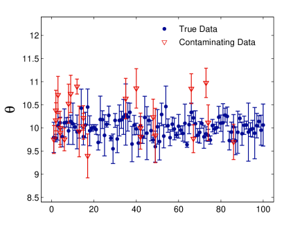
Figure 1: Schematic illustration of the problem: data drawn from the true distribution (e.g. Type Ia supernovae) are contaminated by similar looking data from a different distributions (e.g. Type Ibc or II supernovae) leading to biasing in the best-fit for parameters and in their errors.

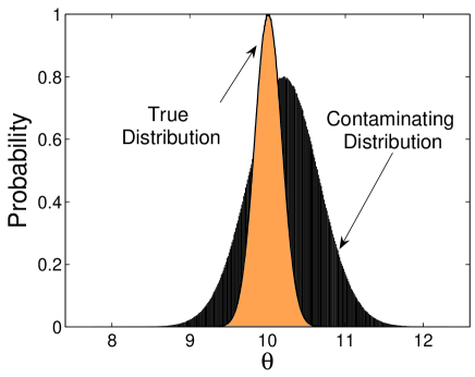
Figure 2: Schematic illustration of the underlying distributions used in Figure (1) for the true and contaminating data. In the case of supernovae, Type Ia have a much more narrow intrinsic scatter in their intrinsic luminosity (narrow Gaussian) compared to other types of supernovae (wide Gaussian) which also have different means.

Until now the choices available in dealing with such a flood of candidates were limited. Either one could limit oneself to those candidates with spectra, rejecting the vast majority of candidates, or one could imagine using the full dataset - including the contaminating data - to perform parameter estimation. However, undertaking this in a naive way - such as simply accepting all candidates which have a probability of being a SNIa greater than some threshold, $P_{*}$ - will lead to significant biases and errors that will undermine the entire dataset.

In contrast, we introduce in this paper a statistically rigorous method for using the candidates without spectroscopic confirmation for parameter estimation. BEAMS offers a fully Bayesian method for appropriately weighting each point based on its probability of belonging to each underlying probability distribution (in the above example, its probability of being a SNIa, SNIbc, type II etc…). We will show that this leads to a parameter estimation method without biases (as long as the method for obtaining the probabilities is sound) and which improves significantly the constraints on (cosmological) parameters.

We will be guided by resolving this specific problem, but the underlying principles and methods are more general and can be applied to many other cases. In order not to obscure the general aspects, we will skip over some details, leaving them for future work where actual supernova data is analysed. We will therefore assume here that we know the redshift of the supernovae (or of its host galaxy), and that we already have estimated the probabilities $P_{j}$ that the j-th supernova is a SN-Ia (eg. by fitting the lightcurves with templates).

To give a simple example, imagine that we wish to estimate a parameter $\theta$ (which in cosmology could for example represent the luminosity distance to a given redshift) from a single data point, $D$, which could have come from one of two underlying classes (e.g. supernova Type Ia or Type II), indexed by $\tau=A,B$ (with their own probability distributions $P(\theta|D,\tau)$, for the parameter $\theta$). Again considering SNe, the link between luminosity and the luminosity distance could be different for the different classes of supernovae due to their intrinsic distribution properties, so given the data $D$, what is the posterior likelihood for $\theta$ assuming that we also know the probability, $P_{\tau}$ that the data point belongs to each class, $\tau$?

Clearly, $P_{A}=1-P_{B}$ since we assume the point could come from only one of two classes. Secondly, as $P_{\tau}\rightarrow 0,1$, the posterior should reduce to one or other of the class distributions. Hence by continuity, the posterior we are seeking should have the form:

$$P(\theta|D)=f(P_{A})P(\theta|D,\tau=A)+g(P_{B})P(\theta|D,\tau=B)$$ (1)

where the continuous functions $f$ and $g$ have the limits $f(0)=0=g(0)$ and $f(1)=1=g(1)$. Since all the posteriors are normalised we have that $\int P(\theta|D)d\theta=1=\int P(\theta|D,\tau)d\theta$. We immediately find that $g(P_{A})=1-f(1-P_{A})$. The simplest – and as we will show later, Bayesian – choice for $f$ is simply the linear function: $f(P_{A})=P_{A}$. In this case the full posterior simply becomes:

$$P(\theta|D)=P_{A}P(\theta|D,\tau=A)+(1-P_{A})P(\theta|D,\tau=B)$$ (2)

This can be easily understood: the final probability distribution for $\theta$ is a weighted sum of the two underlying probability distributions (one for each of the classes) depending on the probabilities $P_{A},P_{B}(=1-P_{A})$ of belonging to each of the two classes.

We will see that our general analysis bears this simple intuition out (see e.g. equation (13)).

II Formalism

II.1 General case

Let us derive in a rather general way the required formulae. Starting from the posterior distribution of the parameters, $P(\theta|D)$ we can work our way towards the known likelihood by repeated application of the sum and product rules of probability theory. The crucial first step involves writing explicitly the marginalisation over different data populations, represented by a logical vector $\tau$. Each entry $\tau_{i}$ is either $A$ if the supernova $i$ is of type Ia, and $B$ if it is not. With each entry we associate a probability $P_{i}$ that $\tau_{i}=A$, so that the probability for $\tau_{i}=B$ is $1-P_{i}$. For now we assume that these probabilities are known. We can then write

$$P(\theta|D)=\sum_{\tau}P(\theta,\tau|D)$$ (3)

where the sum runs over all possible values of $\tau$. Using Bayes theorem we get

$$P(\theta,\tau|D)=P(D|\theta,\tau)\frac{P(\theta,\tau)}{P(D)}.$$ (4)

The “evidence” factor $P(D)$ is independent of both the parameters and $\tau$ and is an overall normalisation that can be dropped for parameter estimation. We will further assume here that $P(\theta,\tau)\approx P(\theta)P(\tau)$. This simplification assumes that the actual parameters describing our universe are not significantly correlated with the probability of a given supernova to be of type Ia or of some other type. Although it is possible that there is some influence, we can safely neglect it given current data as our parameters are describing the large-scale evolution of the universe, while the type of supernova should mainly depend on local gastrophysics. In this case $P(\theta)$ is the usual prior parameter probability, while $P(\tau)$ separates into independent factors,

$$P(\tau)=\prod_{\tau_{i}=A}P_{i}\prod_{\tau_{j}=B}(1-P_{j}),$$ (5)

Here the product over “$\tau_{j}=A$” should be interpreted as a product over those $j$ for which $\tau_{j}=A$. In other words, given a population vector $\tau$ with entries “$A$” for SN-Ia and “$B$” for other types, the total probability $P(\tau)$ is the product over all entries, with a factor $P_{j}$ if the j-th entry is “$A$” and $1-P_{j}$ otherwise (if the j-th entry is “$B$”). Notice that we discuss here only one given vector $\tau$, the uncertainty is taken care of by the outer sum over all possible such vectors. The full expression is therefore

$$P(\theta|D)\propto P(\theta)\sum_{\tau}P(D|\theta,\tau)\prod_{\tau_{i}=A}P_{i}\prod_{\tau_{j}=B}(1-P_{j}).$$ (6)

The factor $P(D|\theta,\tau)$ here is just the likelihood. In general we have to evaluate this expression, which is composed of $2^{N}$ terms for $N$ supernovae. The exponential scaling with the number of data points means that we can in general not evaluate the full posterior – but it should be sufficient to fix $\tau_{i}=A$ for data points with $P_{i}\approx 1$ and $\tau_{j}=B$ for $P_{j}\approx 0$, and to sum over the intermediate cases. This should give a sufficiently good approximation of the the actual posterior.

II.2 Uncorrelated data

In the case of uncorrelated kinds of data or measurements, such as is approximately true for supernovae , we can apply the huge computational simplification pointed out in Press (1996). In this case, the likelihood decomposes into a product of independent probabilities,

$$P(D|\theta,\tau)=\prod_{\tau_{i}=A}P(D_{i}|\theta,\tau_{i}=A)\prod_{\tau_{j}=B}P(D_{j}|\theta,\tau_{j}=B).$$ (7)

The posterior is now a sum over all possible products indexed by the components $\tau_{i}$. We can simplify it, and bring it into a form that lends itself more easily to the extensions considered in a later section, by realising that all binomial combinations can be generated by a product of sums of two terms,

$$\sum_{\tau}\prod_{\tau_{i}=A}A_{i}\prod_{\tau_{j}=B}B_{j}=\prod_{k}(A_{k}+B_{k}).$$ (8)

In this schematic expression, the $A_{i}$ correspond to the product of likelihood and prior for a $\tau_{i}=A$ entry, and the $B_{j}$ to the same product for a $\tau_{j}=B$ entry. So instead of a sum over $2^{N}$ terms, we now only deal with $N$ products.

How do the $A_{k}$ and $B_{k}$ look for our supernova application? Let us assume that we are dealing with two populations, a population $A$ of SNe Ia and population $B$ of non-Ias. For the $k$-th supernova $A_{k}$ is then the product of the probability $P_{k}$ of being type Ia with the likelihood $P(D_{k}|\theta,\tau_{k}=A)$. But since this likelihood is conditional on the supernova being indeed of type Ia, it is just the normal type-Ia likelihood which we will call $\mathcal{L}_{A,k}$. $B_{k}$ on the other hand is the probability $1-P_{k}$ of not being type Ia times the likelihood of the supernovae that are not Ia, which we will call $\mathcal{L}_{B,k}$.

$\mathcal{L}_{A,i}$ is therefore the probability that the $i$-th data point has the measured magnitude if it is type Ia. It is just the usual likelihood, typically taken as a $\chi^{2}$ in the magnitudes. With the $i$-th supernova data given as distance modulus $\mu_{i}$ and total combined error $\sigma_{i}$ (the intrinsic and measurement errors computed in quadrature) it is simply

$$P(D_{i}|\theta,\tau_{i}=1)={\cal L}_{A,i}(\theta)=\frac{1}{\sqrt{2\pi}\sigma_{i}}e^{-\chi_{i}^{2}/2},$$ (9)

with $\chi_{i}^{2}=(\mu_{i}-m(\theta))^{2}/\sigma_{i}^{2}$ where $m(\theta)$ is the theoretical distance modulus (at redshift $z_{i}$). We emphasise that here the normalisation of the likelihood is important – unlike in standard maximum likelihood parameter estimation – as we will be dealing with different distributions and their relative weight depends on the overall normalisation. In the case of SNe we can of course go a level deeper, since the $\mu_{i}$ are estimated from a number of light-curve points in multiple filters. We could start directly with those points as our fundamental data. Here we ignore this complication while noting that in an actual application this would be the optimal approach

The likelihood $\mathcal{L}_{B,i}$ of a non-Ia supernovae is harder. In an ideal world we would have some idea of the distribution of those supernovae, so that we can construct it from there (see e.g. Richardson et al. (2002)). If we do not know anything, we need to be careful to minimise the amount of information that we input. It is tempting to use an infinitely wide flat distribution, but such a distribution is not normalisable. Instead we can assume that the non-Ia points are offset with respect to the “good” data and have some dispersion. The natural distribution given the first two moments (the maximum entropy choice) is the normal (Gaussian) distribution. The potentially most elegant approach is to use the data itself to estimate the width and location of this Gaussian. This is simply done by allowing for a free shift $b$ and width $\Sigma$ and marginalising over them. Optimally we should choose both parameters independently for each redshift bin, in the case where we have many supernovae per bin. Otherwise it may be best consider $b$ as a relative shift with respect to the theoretical value, modelling some kind of bias.

We would like to emphasise that our choice of the normal distribution for the non-Ia points is the conservative choice if we want to add a minimal number of new parameters. It does not mean that we assume it to be the correct distribution. In tests with a uniform and a $\chi^{2}$ type distribution for the non-Ia population, assuming a normal distribution sufficed to reliably remove any bias from the estimation process relying on the Ia data points. If we have a very large number of non-Ia points we could go beyond the normal approximation and try to estimate the distribution function directly, e.g. as a histogram. On the other hand, the more parameters we add, the harder it is to analyse the posterior. Also, if we knew the true distribution of the contaminants then we should of course use this information. Going back to the full likelihood, we now write

$$P(D|\theta,\tau) = \sum_{b,\Sigma}P(D,b,\Sigma|\theta,\tau)$$ (10)

$$= \sum_{b,\Sigma}P(D|b,\Sigma,\theta,\tau)P(b,\Sigma).$$ (11)

The last term is the prior on the non-Ia distribution. In the absence of any information, the conventional (least informative) choice is to consider the two variables as independent, with a constant prior on $b$ and a $1/\Sigma$ prior on the standard deviation. In reality, the sum written here is an integration over the two parameters, and the choice of prior is degenerate with the choice of integration measure. As there are no ambiguities, we will keep using summation symbols throughout, even though they correspond to integrals for continuous parameters.

The type-Ia supernovae are independent of the new parameters. They are only relevant for the non-Ia likelihood, which is now for supernova $j$

$$P(D_{j}|\theta,b,\Sigma,\tau_{j}=B) = {\cal L}_{B,j}(\theta,b,\Sigma)$$ (12)

$$= \frac{1}{\sqrt{2\pi}\Sigma}e^{-\frac{(\mu_{j}-m(\theta)-b)^{2}}{2\Sigma^{2}}}$$

(in an actual application to supernova data we would take $\Sigma$ to be the intrinsic dispersion of the non-Ia population, and add to it the measurement uncertainty in quadrature). The posterior, Eq. (6), is then

$$P(\theta|D)\propto\sum_{b,\Sigma}P(\theta)P(b)P(\Sigma)\times$$

$$\prod_{j=1}^{N}\left\{\mathcal{L}_{A,j}(\theta)P_{j}+\mathcal{L}_{B,j}(\theta,b,\Sigma)(1-P_{j})\right\}$$ (13)

An easy way to implement the sum over $b$ and $\Sigma$ is to include them as normal variables in a Markov-chain monte carlo method, and to marginalise over them at the end. Additionally, their posterior distribution contains information about the distribution of the non-Ia supernovae that can be interesting in their own right.

III A Test-Implementation

In general $\theta$ could of course be a vector of cosmological parameters, but in this section we consider the simple case of the estimation of a constant, corresponding for example to the luminosity distance in a single bin for the SN case. Continuing with the SN example for simplicity, the data $D_{i}$ then corresponds to some $m_{i}$, an apparent magnitude for each SN in a bin. We again assume that there are two populations, type $A$ (corresponding to SNIa) and type $B$ (everything else).

We fix a distribution for the type $A$ probabilities $P_{i}$, for simplicity we take $f(P_{i})\propto P_{i}$, i.e. a distribution that is linearly increasing so that we are dealing predominantly with objects of type $A$. We then draw a $P_{i}$ from this distribution, and choose an actual type with that probability. Finally, we add a “spectroscopic” sample for which $P_{i}=1$, i.e. these are guaranteed to be of type $A$.

We take the type $A$ population to have a known Gaussian distribution with mean $\mu_{A}=0$ and variance $\sigma_{A}=0.1$. The unknown distribution of type $B$ is taken to be another Gaussian, with mean $\mu_{B}=2$ and variance $\sigma_{B}=2$. To all data points, $A$ and $B$, we assign the error bar of type $A$, i.e. $\sigma_{i}=\sigma_{A}$ (but we fit for the error bar of the population $B$). We assume that this error has been derived e.g. from the dispersion of the spectroscopic sample and that we do not know the distribution of the sample $B$ .

The parameters that are being fitted from the data are then $\mu_{A}$, $\mu_{B}$ and $\sigma_{B}$, with $\sigma_{A}$ fixed from the spectroscopic sample, and $P_{i}$ fixed for each point from an assumed previous step in the analysis (e.g. $P_{i}$ obtained from goodness of fit to template lightcurves). As a side remark, although $\sigma_{A}$ is here assumed to be known from the dispersion of the spectroscopic sample, it can also be fitted for jointly with the other parameters, which was done in tests of the method ; the assumption of fixed known $P_{i}$ will be relaxed in later sections. To connect this highly simplified example with cosmology, we shall pretend that we consider here only one redshift bin, and that the same analysis is repeated for each bin. The value of $\mu_{A}$ could then be the distance modulus $\mu$ in one bin, and an unbiased estimate in all bins would then constrain cosmological parameters like $\Omega_{m},\Omega_{\Lambda}$ etc. The smaller the errors on $\mu_{A}$, the better the constraints. The data from population $B$ on the other hand give us no information on the distance modulus, hence we must reduce contamination from population $B$. The posterior that results (explicitly indicating that we estimate $\mu_{A}$) is then

$$P(\mu_{A}|D,\sigma_{A})\propto\sum_{\mu_{B},\sigma_{B}}\frac{1}{\sigma_{B}}\times$$

$$\prod_{j=1}^{N}[P_{j}{\cal L}_{A,j}(\mu_{A},\sigma_{A})+(1-P_{j}){\cal L}_{B,j}(\mu_{B},\sigma_{B})],$$ (14)

where the population $B$ mean $\mu_{B}$ and the variance $\sigma_{B}$ have taken over the role of the shift $b$ and variance $\Sigma$ of the last section.

As the population $B$ is strongly biased with respect to $A$, the algorithm needs to detect the type correctly to avoid wrong results. Table 1 shows results from an example run with the above parameters, $10$ spectroscopic and $1000$ photometric data points, where the spectroscopic points are data generated in a Monte Carlo fashion from normally distributed population $A$ and the photometric data consist of points from both population $A$ and population $B$ with associated probabilities $P_{i}\leq 1$. In this table and all following tables we add a “Bias” column that shows the deviation of the recovered parameters from the input values in units of standard deviations.

Parameter	Value	Bias [$\sigma$]
$\mu_{A}$	$-0.003\pm 0.004$	$0.8$
$\mu_{B}$	$2.00\pm 0.11$	$0.0$
$\sigma_{B}$	$1.90\pm 0.07$	$1.4$

Table 1: Example results for the basic algorithm applied to a sample of $10$ “spectroscopic” and $1000$ “photometric supernovae” in a bin. The bias column shows the deviation from the true value, in units of the standard deviation. A deviation of about $1\sigma$ is expected, while about one in twenty realisations is more than $2\sigma$ away for random data with normal distribution. BEAMS also allows to recover the parameters characterising the contaminating distribution, $\mu_{B}$ and $\sigma_{B}$.

For the spectroscopic sample the errors just scale like $\sigma_{A}/\sqrt{N}$. Each of the other supernova contributes to the “good” measurement with probability $P_{j}$, i.e. each data point has a weight $P_{j}$, or an effective error bar $\sigma_{A}/\sqrt{P_{j}}$ on average. Defining the average weight

$$w\equiv\frac{1}{N}\sum_{j=1}^{N}P_{j}\rightarrow\int d\!PPf(P)=\langle P\rangle$$ (15)

where $f(P)$ is the normalised probability distribution function of the $P_{j}$, we find that the error on $\mu$ scales as

$$\sigma_{\mu}=\frac{\sigma_{A}}{\sqrt{N_{s}+wN_{ph}}}$$ (16)

for $N_{s}$ spectroscopic measurements ($P_{j}=1$) and $N_{ph}$ uncertain (photometric only) measurements with average weight $w$. As can be seen in Fig. 3, the errors on $\mu$ recovered by the Bayesian formalism do indeed follow this formula, although they can be slightly worse if the two populations are more difficult to separate than in this example.

In our example where $f(P_{j})\propto P_{j}$ the weight is $w=2/3$, so that three photometric supernovae equal two spectroscopic ones. The expected error in $\mu_{A}$ for the example of table 1 is therefore $0.1/\sqrt{10+2/3\times 1000}\approx 0.004$, in agreement with the numerical result. If we had used only the $10$ spectroscopic data points, the error would have been $0.032$ so that the use of all available information improves the result by a factor eight. In the case where $f(P_{i})\propto(1-P_{i})$, i.e. we are dealing predominantly with type $B$ data, we have a weight of $1/3$. If it is easier to measure three photometric supernovae compared to one spectroscopic one, it will still be worth the effort in this case. We should point out here that these are the optimal errors achievable with the data. In Fig. 3 we show the actual recovered error from random implementations with different $w$ and effective number of SNIa given by:

$$N_{\mathrm{eff}}\equiv N_{s}+wN_{ph}\,.$$ (17)

We see that the Bayesian algorithm achieves nearly optimal errors (black line).

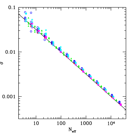
Figure 3: Scaling of the errors: The black line shows the expected (optimal) error, which is inversely proportional to the effective number of SNIa given by $\sqrt{N_{\mathrm{eff}}}$ in eq. (17). The different colours and shapes correspond to different distributions of the probabilities $P_{i}$ (i.e. how many data points have $P_{i}=0.9$, how many have $P_{i}=0.8$, etc.). The points show the actually measured error for BEAMS given these distributions of the probabilities $P_{i}$ of the data. BEAMS is able to use nearly all of the information available.

We now compare the Bayesian method to some other possible methods:

• Use only spectroscopic SNIa.

• Use only SNIa with probabilities above a certain limiting threshold, $P$. A limit of $0\%$ uses all data points, and a limit of $100\%$ only the spectroscopically confirmed points.

• Weight the $\chi_{i}^{2}$ value for the $i$-th point by a function of $P_{i}$. This effectively corresponds to increasing the error for data points with lower probability. For the test, we use the weighting $\sigma_{j}\rightarrow\sigma_{j}/P_{j}^{N/2}$. For $N=0$ this reverts to the limiting case where we just use all of the data in the usual way. For $N>0$ points are progressively more and more heavily penalised for having low probabilities.

These ad-hoc prescriptions are not necessarily the only possibilities, but these were the methods we came up with for testing BEAMS against. We now discuss their application to the same test-data described above to see how they perform against BEAMS.

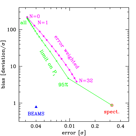
Figure 4: A comparison between different methods (see text). Of these methods, only the BEAMS method and the use of the spectroscopic points alone are unbiased. As it can use the uncertain data, the BEAMS method improves the error bars in this example by the (expected) factor of $8$. (For the error-weighted method not all values of $N$ were plotted at the high-N end.)

Figure 4 shows very clearly that although the ad-hoc prescriptions for dealing with the type-uncertainty can lead to very precise measurements, they cannot do so without being very biased. Both the Bayesian and the pure-spectroscopic approach recover the correct value (bias less than one $\sigma$), but the latter does so at the expense of throwing away most of the information in the sample.

We can also use BEAMS to get a posterior estimate of the population type, based on the prior value (e.g. from multicolour light curves) and the distribution. To do this for data point $j$ we marginalise over all entries $\tau$ except $\tau_{j}$, and additionally over all estimated parameters. In practice this means that the $j-th$ entry in Eq. (14) is fixed to $\mathcal{L}_{A,j}$, and that we also integrate over $\mu_{A}$ in addition to $\mu_{B}$ and $\sigma_{B}$. Effectively, we compute the model probability if the $j$-th point is assumed to be of type $A$ and compare it to the model probability without this constraint. The relative probability of the two cases then tells us the posterior probability for the model vector $\tau$ having the $j$-th entry equal to $A$, corresponding to the posterior probability of the $j$-th supernova to be of type $A$. Fig. 5 shows an example case (using a Gaussian approximation to evaluate the integral over all values of the sample mean $\mu_{A}$). We see how the posterior probability to belong to population $A$ depends both on how well the location of a point agrees with the distribution of $A$ (left) and on how high its prior probability was (right). In other words, we can reconstruct which points came from which distribution from the agreement between their values of $\mu$ and $\mu_{A}$ and their prior probabilities (which is indeed all the information at our disposal in this scenario).

For the toy example the two distributions are quite different, and BEAMS classifies all points within about $3\sigma$ of $m=0$ to be of population $A$. The prior probability is here strongly overwhelmed by the data and the resulting posterior probabilities lie close to $0$ and $1$ for most data points.

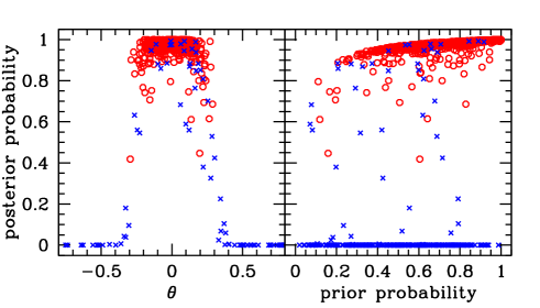
Figure 5: BEAMS as a classification algorithm: we plot the posterior probability of the data points to be of type $A$ in our toy example. This depends on their value $m_{j}$ (left panel) and their prior probability (right panel). The better a point agrees with the recovered distribution of type $A$, the higher its posterior probability to belong to it. See text for more information. For this test case we know the true nature of the points, and plot population $A$ as red circles and population $B$ as blue crosses (see Table 1 for distribution characteristics). .

In the following section we extend this basic model in two main directions. Firstly, as reality starts to deviate from the model, there is a danger of introducing a bias. We discuss a few simple cases and try to find ways of hardening the analysis against the most common problems. Secondly, we extend the model to more than two families, and we also discuss the possibility of using the information on the other populations in the analysis itself.

IV Extensions

IV.1 Uncertain probabilities

While the likelihoods used in the estimation of $\mu_{A}$ (which will yield $\theta$) are the same for the earlier example, in this section our treatment and use of the probabilities $P_{i}$ differs as we begin to include possible error in the $P_{i}$’s.

Often one may not know the population probability $P_{j}$ precisely, but has instead a probability distribution. For example $P_{j}$ may be roughly known, but has an error associated with it (in the SN case this could be due to some systematics in the lightcurve fitting process). In this case we have to marginalise over all those probability distributions. For $N$ supernovae this then requires an $N$-dimensional integration. It is straightforward to include this in a MCMC approach by allowing all $P_{j}$ to be free variables, but with $N$ of the order of several thousand it may be difficult to get a precise result. On the other hand this may still be better than just sampling $P_{j}$ at a single point if it is not known exactly.

However, if the measurements are independent, then each integral affects only one of the terms in the product over all data points in Eq. (13). Instead of one $N$ dimensional integration we are dealing with $N$ one-dimensional integrations which are much easier to compute. In general we have to integrate each term over the probability $p_{j}$ with a given distribution $\pi(p_{j})$. The case of a known probability corresponds to $\pi(p_{j})=\delta(p_{j}-P_{j})$. The next simplest example is the case of a totally unknown probability $P_{j}$, for which $\pi(p_{j})=1$. In this case the integral to be solved in each term is

$$\int dp_{j}\left({\cal L}_{A,j}p_{j}+{\cal L}_{B,j}(1-p_{j})\right)=\frac{1}{2}({\cal L}_{A,j}+{\cal L}_{B,j}),$$ (18)

where ${\cal L}_{A,j}$ and ${\cal L}_{B,j}$ are the likelihood values of the $j$-th data point assuming population $A$ or $B$ respectively. The effective probability here turns out to be $P_{j}=1/2$. The reason is that we estimate this probability independently for each supernova, and do not have enough information to estimate it from the data. In the following subsection we replace this approach instead with a global uncertain probability added to the known distributions. This global probability can then be estimated from the data.

For now, assume we have an approximate knowledge of the type-probabilities, say, an independent uncertainty on each $P_{j}$, $\delta_{j}$, so that

$$\pi(p_{j})\propto e^{-\frac{(p_{j}-P_{j})^{2}}{2\delta_{j}^{2}}},$$ (19)

where the proportionality constant is chosen so that the integral over $\pi(p_{j})$ from zero to one is $1$. If the random error on $P_{j}$ is small enough that the distribution function is well contained within the domain of integration, i.e. $P_{j}+\delta_{j}\ll 1$ and $P_{j}-\delta_{j}\gg 0$, then we recover just $p_{j}=P_{j}$. In this case the Gaussian distribution function acts effectively as a delta-function. For large uncertainties, or for probabilities close to the boundaries, corrections will become important and can bias the result. For the specific case of random errors, the correction term is of the form $\mathcal{L}_{A,j}-\mathcal{L}_{B,j}$. If we suspect large random errors it may be worth adding this term with a global pre-factor of its own to the full posterior. On the other hand, in real applications we expect that the probabilities close to $P_{j}=1$ are quite well known, so that the boundary error is hopefully not too important.

A fixed, common shift is much more worrying and can bias the results significantly. This can be seen in table 2 where we added a systematic shift to the probabilities (enforcing $0\leq P_{j}\leq 1$). This is an especially important point for photometric supernova analyses, where dust reddening can bias the classification algorithm. If we do not take into account this possibility, then the analysis algorithm fails because it starts to classify the supernovae wrongly, but hopefully such a large bias is unrealistic.

shift of $P_{j}$	$\mu_{A}$	Bias [$\sigma$]
$+0.1$	$0.021\pm 0.004$	$~{}5.5$
$+0.2$	$0.128\pm 0.004$	$31.8$
$+0.4$	$0.408\pm 0.004$	$96.8$
$-0.4$	$0.003\pm 0.005$	$~{}0.6$

Table 2: Results with a systematic shift (i.e. bias) in the probabilities $P_{j}$. Positive shifts lead to a systematic bias in the results, while negative shifts lead to sub-optimal errors. However, the negative shifts will bias instead the inferred properties of population B.

At any rate, a bias is readily dealt with by including a free (global) shift $s$ into the probability factors of Eq. (13) and by marginalising over it, resulting in

$$P(\mu_{A},\mu_{B},\sigma_{B}|D)\propto$$

$$\sum_{s}\frac{1}{\sigma_{B}}\prod_{j=1}^{N}\left[{\cal L}_{A,j}(P_{j}+s)+{\cal L}_{B,j}(1-P_{j}-s)\right].$$ (20)

It may be a good idea to include such a shift and to check its posterior distribution. Given enough data it does not significantly impact the errors, and it adds stability also in the case of large random uncertainties in the $P_{j}$. We found that an additive bias with a constant prior was able to correct all biasing models that we looked at, as is shown in table 3. However, the presence of a significant shift would indicate a failure of the experimental setup and should be taken as a warning sign.

A free individual shift is degenerate with the case of random uncertainties above, as it cannot be estimated from the data, and is not very useful in this context.

shift of $P_{j}$	$\mu_{A}$	Bias [$\sigma$]	recovered shift
$+0.0$	$-0.003\pm 0.004$	$-0.8$	$\hphantom{-}0.002\pm 0.011$
$+0.1$	$-0.004\pm 0.004$	$-1.0$	$\hphantom{-}0.073\pm 0.012$
$+0.2$	$-0.000\pm 0.004$	$-0.1$	$\hphantom{-}0.158\pm 0.015$
$+0.4$	$-0.002\pm 0.004$	$-0.6$	$\hphantom{-}0.286\pm 0.016$
$-0.4$	$\hphantom{-}0.004\pm 0.004$	$\hphantom{-}1.0$	$-0.396\pm 0.013$

Table 3: Same as table 2, but the model allows for a bias (shift) in the $P_{j}$. As most supernovae are population A, with $f(P_{j})\propto P_{j}$, the recovered shift grows slower than the input shift. However, it still removes any bias in the estimation of $\mu_{A}$.

IV.2 Global uncertainty

Given how critical the accuracy of the type-probability $P_{j}$ is in order to get correct results, it may be preferable, as an additional test, to discard this information completely. This helps to protect against wrongly classified outliers and the unexpected breakdown or biasing of the classification algorithm.

Even if the probability for a supernova to be either of type Ia or of another type is basically unknown, corresponding to a large error on all the $P_{i}$, not all is lost. We can instead include a global probability $p$ that supernovae belong to either of the groups, and then marginalise over it. In this way, the data will pick out the most likely value for $p$ and which observations belong to which class. In terms of the posterior (13) this amounts just to replacing all $P_{j}$ with $p$ and to marginalise over it,

$$P(\mu_{A},\mu_{B},\sigma_{B}|D)\propto$$

$$\sum_{p}P(p)\frac{1}{\sigma_{B}}\prod_{j=1}^{N}\left\{\mathcal{L}_{A,j}p+\mathcal{L}_{B,j}(1-p)\right\}.$$ (21)

The prior on $p$, $P(p)$, contains any knowledge that we have on the probability that any given supernova in our survey is of type Ia. If we do not know anything then a constant prior works well. As this is a global probability (i.e. all supernovae have the same $p$), we cannot in this form include any “per supernova” knowledge on $p$, gained for example from spectra or light curves. For this we need to revert to the individual probabilities discussed previously. However, it is a good idea to include the spectroscopic (known to be good) points with an explicit $p=1$ as they then define which population is the “good” population and generally make the algorithm more stable.

shift of $P_{j}$	$\mu_{A}$	Bias [$\sigma$]	global probability
$+0.0$	$-0.003\pm 0.004$	$-0.8$	$0.66\pm 0.02$
$+0.1$	$-0.004\pm 0.004$	$-0.9$	$0.68\pm 0.02$
$+0.2$	$\hphantom{-}0.000\pm 0.004$	$\hphantom{-}0.0$	$0.66\pm 0.02$
$+0.4$	$-0.003\pm 0.004$	$-0.7$	$0.64\pm 0.02$
$-0.4$	$\hphantom{-}0.004\pm 0.004$	$\hphantom{-}0.9$	$0.65\pm 0.02$

Table 4: Same as table 2, but the model uses an estimated global probability $p$ for all supernovae and does not use the $P_{j}$ (so in reality all runs above are the same). The expected global probability is $p=N_{\mathrm{eff}}/N\approx 0.66$.

In our numerical tests with the toy model described in section III this approach works very well, see table 4. However if the two distributions are difficult to separate, with similar average and dispersion, then the algorithm can no longer distinguish between them and concludes that the data is compatible with having been drawn from a single distribution with averaged properties. This does normally not lead to a high bias, since otherwise the data would have been sufficient to tease the populations apart. Nevertheless, it seems preferable to use the relative probabilities for the supernova types when the information is available and reliable.

IV.3 Several populations

For an experiment like the SDSS supernova survey, a more conservative approach may be to add an additional population with a very wide error bar that is designed to catch objects that have been wrongly classified as supernovae, or those which got a very high Ia probability by mistake.

Of course there is no reason to limit ourselves to two or three populations, given enough data. If we end up with several thousand supernovae per bin we can try to use the data itself to understand the different sub-classes into which the supernovae can be divided.

The expression (13) can be straightforwardly generalised to $M$ classes $A_{i}$ of objects (for example supernova types) with their own means $\mu_{i}$ and and errors $\sigma_{i}$ as well as the probability for data point $j$ to be in class $A_{i}$ of $P_{j}^{i}$,

$$P(\mu_{i},\sigma_{i}|D)\propto\frac{1}{\prod_{i=1}^{M}\sigma_{i}}\prod_{j=1}^{N}\left\{\sum_{i=1}^{M}\mathcal{L}_{i,j}(\mu_{i},\sigma_{i})P_{j}^{i}\right\}.$$ (22)

For each data point $j$ the probabilities have to satisfy $\sum_{i}P_{j}^{i}=1$. Of course there has to be at least one class for which the model is known, i.e. for which we know the connection between $\mu_{i}$ and the (cosmological) parameter vector $\theta$ (the “Ia” class in the supernova example), or else it would not be possible to use this posterior for estimating the model parameters $\theta$ and we end up with a classification algorithm instead of constraining cosmology.

It is possible that we even do not know how many different populations to expect. In this case we can just keep adding more populations to the analysis. We should then also compute the evidence factor as a function of the number $M$ of populations, $P(D|M)$, by marginalising the posterior of Eq. (4) over the parameters,

$$P(D|M)=\sum_{\theta,\tau}P(D|\theta,\tau)P(\theta,\tau).$$ (23)

This is just the integral over all $\mu_{i}$ and $\sigma_{i}$ of the “posterior” that we have used so far, Eq. (22), since we did not normalise it. Once we have computed this factor, then we can compare the relative probabilities of the number of different populations by comparing their evidence factor, since by Bayes theorem (again),

$$P(M|D)=P(D|M)\frac{P(M)}{P(D)}.$$ (24)

The relative probability of models with $m_{1}$ and $m_{2}$ populations is then

$$\frac{P(D|m_{1})}{P(D|m_{s})}\frac{P(m_{1})}{P(m_{2})}$$ (25)

and usually (in absence of additional information) the priors are taken to be $P(m_{1})=P(m_{2})$ so that the evidence ratio gives directly the relative probability.

IV.4 Combined Formula

What is the best way to combine the above approaches for future supernova surveys? There is probably no “best way”. For the specific example of the SDSS supernova survey the probabilities for the different SN populations are derived from $\chi^{2}$ fits to lightcurve templates Sullivan et al. (2006). We expect three populations, Ia, Ibc and II, and objects that are not supernovae at all. We expect that last class to be very inhomogeneous, but we would like to keep the supernovae. From the spectroscopically confirmed supernovae we can learn what the typical goodness-of-fit of the templates is expected to be and so calibrate them. Supernovae where the $\chi^{2}$ of all fits is, say, $10$ higher than for the typical spectroscopic cases are discarded. For the reminder we set $\pi_{i}=\exp(-(\chi_{0}^{2}-\chi^{2})_{i}/2)$ where $\chi_{0}^{2}$ is the typical value for each population. If $\sum_{i}\pi_{i}>1$ then we set the probabilities to be $P_{j}=\pi_{j}/\sum_{i}\pi_{i}$, otherwise $P_{j}=\pi_{j}$. We also write again the more general $\theta$ for the parameters of interest. $\theta$ can represent for example cosmological parameters, or the luminosity distance to a redshift bin. The connection between $\theta$ and the data is specified in the likelihoods $P(D_{j}|\theta,\ldots)$ which in general compare the measured magnitude to the theoretical value, with the theoretical value depending on the $\theta$, in other words $P(D_{j}|\theta,\mathrm{Ia})=\mathcal{L}_{\mathrm{Ia},j}(\theta)$, and so on. The full formula then is

$$P(\theta|D) \propto \sum_{b_{k},\Sigma_{k}}P(\theta)P(b)P(\Sigma)\times$$

$$\prod_{j=1}^{N}\Large\{P(D_{j}|\theta,\mathrm{Ia})P(\mathrm{Ia})_{j}$$

$$+P(D_{j}|\theta,b_{\mathrm{Ibc}},\Sigma_{\mathrm{Ibc}},\mathrm{Ibc})P(\mathrm{Ibc})_{j}$$

$$+P(D_{j}|\theta,b_{\mathrm{II}},\Sigma_{\mathrm{II}},\mathrm{II})P(\mathrm{II})_{j}$$

$$+P(D_{j}|\theta,b_{X},\Sigma_{X},X)$$

$$\times(1-P(\mathrm{Ia})_{j}-P(\mathrm{Ibc})_{j}-P(\mathrm{II})_{j})\Large\}$$

If on the other hand we do not trust the absolute values of the $\chi^{2}$ then we can either add a bias to safeguard against a systematic shift in the absolute probabilities, or allow for a global $P_{X}$ that an object is no supernova at all. For this we always normalise the supernova probabilities to unity, $P_{j}=\pi_{j}/\sum_{i}\pi_{i}$, and use the likelihood

$$P(\theta|D) \propto \sum_{b_{k},\Sigma_{k},P_{X}}P(\theta)P(b)P(\Sigma)P(P_{X})\times$$

$$\prod_{j=1}^{N}\Large\{\Large[P(D_{j}|\theta,\mathrm{Ia})P(\mathrm{Ia})_{j}$$

$$+P(D_{j}|\theta,b_{\mathrm{Ibc}},\Sigma_{\mathrm{Ibc}},\mathrm{Ibc})P(\mathrm{Ibc})_{j}$$

$$+P(D_{j}|\theta,b_{\mathrm{II}},\Sigma_{\mathrm{II}},\mathrm{II})P(\mathrm{II})_{j}\Large](1-P_{X})$$

$$+P(D_{j}|\theta,b_{X},\Sigma_{X},X)P_{X}\Large\}$$

It is probably a good idea to always run an analysis with additional safeguards like this, and preferably a free global bias in the Ia probability, in parallel to the “real” analysis in case something goes very wrong. The global bias $\Delta$ might be added as

$$P(\theta|D) \propto P(\theta)\!\!\!\!\!\!\!\!\sum_{b_{k},\Sigma_{k},\Delta_{i},P_{X}}\!\!\!\!\!\!\!\!P(P_{X})\!\!\!\!\!\!\!\!\prod_{k\in\{\mathrm{Ibc},\mathrm{II},X\}}\!\!\!\!\!\!\!\!P(b_{k})P(\Sigma_{k})\prod_{i=1}^{2}P(\Delta_{i})\times$$

$$\prod_{j=1}^{N}\Big{\{}\Big{[}P(D_{j}|\theta,\mathrm{Ia})\left[P(\mathrm{Ia})_{j}-\Delta_{1}-\Delta_{2}\right]$$

$$+P(D_{j}|\theta,b_{\mathrm{Ibc}},\Sigma_{\mathrm{Ibc}},\mathrm{Ibc})\left[P(\mathrm{Ibc})_{j}+\Delta_{1}\right]$$

$$+P(D_{j}|\theta,b_{\mathrm{II}},\Sigma_{\mathrm{II}},\mathrm{II})\left[P(\mathrm{II})_{j}+\Delta_{2}\right]\Big{]}(1-P_{X})$$

$$+P(D_{j}|\theta,b_{X},\Sigma_{X},X)P_{X}\Big{\}},$$

Especially the bias $\Delta_{2}$ of the Ia vs II probability is useful to catch problems due to dust-reddening which can lead to a confusion between these two classes Poznanski et al. (2002).

While estimating a dozen additional parameters is not really a problem statistically if we have several thousand data points, it can become a rather difficult numerical problem which justifies some work in itself. We are using a Markov-chain monte carlo code with several simulated annealing cycles to find the global maximum of the posterior, which seems to work reasonably well but could certainly be improved upon.

We notice that in addition to a measurement of the model parameters $\theta$ from the Ia supernovae, we also get estimates of the distributions of the other populations. In principle we could feed this information back into the analysis. Even though the prospect of being able to use the full information from all data points is very tempting, we may not win much from doing so. We would expect that the type-Ia supernovae are special in having a very small dispersion in the absolute magnitudes. As such, they carry a lot more information than a population with a larger dispersion. In terms of our toy-example where $\sigma_{A}=0.1$ and $\sigma_{B}=2$ we need $(\sigma_{B}/\sigma_{A})^{2}=400$ times more population $B$ points to achieve the same reduction in the error. Unless we are lucky and discover another population with a very small dispersion (or a way to make it so), we expect that the majority of the information will always come from the SNIa.

V Conclusions

We present a generalised Bayesian analysis formalism called BEAMS (Bayesian Estimation Applied to Multiple Species) that provides a robust method of parameter estimation from a contaminated data set when an estimate of the probability of contamination is provided. The archetypal example we have in mind is cosmological parameter estimation from Type Ia supernovae (SNIa) lightcurves which will inevitably be contaminated by other types of supernovae. In this case lightcurve template analysis provides a probability of being a SNIa versus the other types.

We have shown that BEAMS allows for significantly improved estimation when compared to other estimation methods, which introduce biases and errors to the resulting best-fit parameters.

BEAMS applies to the case where the probability, $P_{i}$, of the $i$-th point belonging to each of the underlying distributions is known. Where the data points are independent, repeated marginalisation and application of Bayes’ theorem yields a posterior probability distribution that consists of a weighted sum of the underlying likelihoods with these probabilities. Although the general, correlated, case where the likelihood does not factor into a product of independent contributions is simple to write down, it contains a sum over $2^{N}$ terms (for 2 populations and $N$ data points). This exponential scaling makes it unsuitable for application to real data where $N$ is easily of the order of a few thousand. This case will require further work.

We have studied in some detail the simple case of estimating the luminosity distance in a single redshift bin from one population consisting of SNIa candidates and another of non SNIa candidates. In addition to an optimal estimate of the luminosity distance, by including the free shift $b$ and width $\Sigma$ of the wide Gaussian distribution as variables in the MCMC estimation method, the BEAMS method also allows one to gain insight into the underlying distributions of the contaminants themselves, which is not possible using standard techniques. Provided that the model for at least one class of data are known, this method can be expanded to more distributions, each with their own shift $b_{i}$ and width $\Sigma_{i}$.

BEAMS was tested against other methods, such as using only a spectroscopically confirmed data set in a $\chi^{2}$ analysis; using only data points with probabilities higher than a certain cut off value, and weighting a $\chi^{2}$ value by some function of the probability. The Bayesian method performs significantly better than the other methods, and provides optimal use of the data available. In the SNe Ia case, the Bayesian framework provides an excellent platform for optimising future surveys, which is specifically valuable given the high costs involved in the spectroscopic confirmation of photometric SNe candidates.

A Bayesian analysis is optimal if the underlying model is the true model. Unfortunately in reality we rarely know what awaits us, and it is therefore a good idea to add some extra freedom to the analysis, guided by our experience. In this way BEAMS can also be applied when the population probability is not known precisely. In this case a global uncertainty is added to the known probability distributions, which can be estimated from the data. In the case of the SNe Ia, one can include a global probability $p$ that the supernovae belong to either group, and then marginalise over it, allowing the data to not only estimate the most likely value for $p$ but also to separate the data into the two classes. This global approach can protect against outliers when the accuracy of the type-probability is not known precisely. It is one of the strengths of Bayesian approaches that they allow one to add quite general deviations from perfect data, which are then automatically eliminated from the final result, and to compute the posterior probability that such surprises were present.

A robust method of application of BEAMS to data from future supernova surveys is proposed to estimate the properties of the contaminant distributions from the data, and to obtain values for the desired parameters. Although we have illustrated and developed the BEAMS algorithm here with explicit references to a cosmological application, it is far more general. It can be easily applied to other fields, from photometric redshifts to other astronomical data analyses and even to other fields like e.g. biology. Since it is Bayesian in nature, it can very easily be tailored to the specific needs of a subject, through simple and straightforward calculations.