The Ophiuchus Superbubble: A Gigantic Eruption from the Inner Disk of the Milky Way

Abstract

While studying extraplanar neutral hydrogen in the disk-halo transition of the inner Galaxy we have discovered what appears to be a huge superbubble centered around $\ell\approx 30\arcdeg$, whose top extends to latitudes $>25\arcdeg$ at a distance of about 7 kpc. It is detected in both H I  and H$\,\alpha\>$. Using the Green Bank Telescope of the NRAO, we have measured more than 220,000 H I  spectra at $9\arcmin$ angular resolution in and around this structure. The total H I  mass in the system is $\approx 10^{6}$ $M_{\sun}$ and it has an equal mass in H${}^{+}\>$. The Plume of H I  capping its top is $1.2\times 0.6$ kpc in $\ell$ and $b$ and contains $3\times 10^{4}$ $M_{\sun}$ of H I  . Despite its location, (the main section is 3.4 kpc above the Galactic plane) the kinematics of the Plume appears to be dominated by Galactic rotation, but with a lag of 27 km s${}^{-1}\>$from corotation. At the base of this structure there are “whiskers” of H I  several hundreds of pc wide, reaching more than 1 kpc into the halo; they have a vertical density structure suggesting that they are the bubble walls and have been created by sideways rather than upwards motion. They resemble the vertical dust lanes seen in NGC 891. From a Kompaneets model of an expanding bubble, we estimate that the age of this system is $\approx 30$ Myr and its total energy content $\sim 10^{53}$ ergs. It may just now be at the stage where its expansion has ceased and the shell is beginning to undergo significant instabilities. This system offers an unprecedented opportunity to study a number of important phenomena at close range, including superbubble evolution, turbulence in an H I  shell, and the magnitude of the ionizing flux above the Galactic disk.

1 INTRODUCTION

A key factor in Galactic evolution is the very complex interaction between stellar evolution and the interstellar medium. Stellar winds and supernovae not only redistribute hydrogen and heavy elements, but in sufficient quantity, can totally shut down star formation by moving gas to the intergalactic medium. In addition, circulation of gas from the disk into the halo, or accretion of low-metallicity gas, will alter the chemical evolution of the Galaxy (Veilleux et al. (2005) and references therein; Sancisi (1999); Tripp et al. (2003)).

The Milky Way offers a unique yet often confused perspective on these processes. Neutral, warm, and hot gas is observed far from the Galactic plane, and ‘superbubbles’ are sometimes seen surrounding sites of recent star formation, though the connection between the different phases, and indeed the differentiation between local, Galactic halo, and intergalactic phenomena is not always clear.

A search for shells and shell-like structures in the Milky Way was completed by Heiles (1979, 1984), complemented by Hu (1981) at high Galactic latitudes and by McClure-Griffiths et al. (2002) in the southern hemisphere. Recently an automated search for shells in the Leiden-Dwingeloo survey (Hartmann & Burton, 1997) was carried out by Ehlerová & Palouš (2005), who discovered nearly 300 structures, several of which were identified with objects from Heiles’ and Hu’s catalogs. Shells and supershells are also observed in nearby galaxies including M31, the LMC and the SMC (Brinks & Bajaja, 1986; Kim et al., 1999; Staveley-Smith et al., 1997; Stanimirovic et al., 1999; Walter & Brinks, 1999; Howk & Savage, 2000). Heiles (1984) and McClure-Griffiths et al. (2002) thoroughly analyze a few specifically chosen shells from their surveys (see also McClure-Griffiths et al., 2000). Recent examples of studies of individual shells are: Aquilla Supershell: Maciejewski et al. (1996); Scutum Supershell: Callaway et al. (2000) (in H I  , H$\,\alpha\>$, infrared, X-ray and UV), Savage et al. (2001) (UV-absorption).

The simplest spherically-symmetric self-similar theory of the superbubbles was developed by Pikel’ner & Shcheglov (1969), Castor et al. (1975) and Weaver et al. (1977), among others. Koo & McKee (1992a, b) gave the problem of spherically-symmetric bubble a more general analytical treatment, and Oey & Clarke (1997) used the self-similar approach to derive the size distribution of shells in a galaxy; their results are in good agreement with observations of nearby galaxies. Based on an early approach of Kompaneets (1960), a 2D semi-analytical model of a bubble in a stratified medium was developed by Mac Low & McCray (1988). Tomisaka & Ikeuchi (1986); Mac Low et al. (1989); Tenorio-Tagle et al. (1987, 1990); Igumenshchev et al. (1990) gave the 2D problem a numerical treatment. Mac Low et al. (1989) found the results of approximate Kompaneets-model calculations to be in excellent agreement with their exact numerical solutions. A detailed review of early theoretical and observational work on superbubbles was given by Tenorio-Tagle & Bodenheimer (1988). A detailed critical analysis of the Kompaneets approximation was given by Koo & McKee (1990), who showed how this method can be improved. The complete range of approximate superbubble models was reviewed by Bisnovatyj-Kogan & Silich (1995).

A number of 3D numerical treatments of the superbubble problem have now been done: Tomisaka (1998) studied how a Galactic magnetic field changes the traditional 2D numerical results; Korpi et al. (1999) simulated superbubbles with a non-ideal MHD model; de Avillez & Berry (2001) carried out a high-resolution hydrodynamical study and their approach was expanded by Breitschwerdt & de Avillez (2006) to model the Local and Loop I bubbles.

In a recent discussion Oey (2004) finds the conventional superbubble paradigm to be consistent with the observational data. A few problems exist, the most serious of which is the “energy-deficit problem” (Oey & García-Segura, 2004; Cooper et al., 2004), but there is nothing which suggests that the basic theory is in error.

New studies in directions where one might have some hope of untangling the different processes and understanding their relationships may yield interesting results. To this end we have been measuring the disk-halo transition of the Milky Way in the 21 cm line of H I  , using the Green Bank Telescope to map neutral gas above the Galactic plane in the inner Galaxy. The power of this telescope is such that significant new insights into Galactic H I  can be obtained with integration times as short as two seconds per spectrum. We have focussed our first efforts on regions near the tangent points in the first longitude quadrant of the inner Galaxy, where Galactic rotation is projected entirely along the line of sight and the distance to the highest velocity features can be estimated with a reasonable degree of accuracy. This paper reports the discovery of a very large, coherent H I  structure which extends $>3$ kpc into the Galactic halo near the tangent point at $\ell=30\arcdeg$, and which is likely to be a relatively nearby example of the superbubbles playing a critical role in galaxy evolution. It lies predominantly in the Ophiuchus constellation, so we refer to it as the Ophiuchus superbubble.

In section 2 of this paper we describe the H I  observations and in section 3 the corresponding data reduction; section 4 summarizes the observed properties of the superbubble in both H I  and H$\,\alpha\>$. In section 5 we discuss the distance to the system and derive some of its physical properties. Section 6 tests the validity of the superbubble hypothesis against a simple analytical model, which also provides estimates of the age and energetics of the system, and in section 7 possible sources of the superbubble’s origin and ionization are considered. Section 8 concludes the paper with a general discussion of the results.

2 OBSERVATIONS

The observations were made with the National Radio Astronomy Observatory’s 100 m diameter Robert C. Byrd Green Bank Telescope (GBT). The angular resolution of the telescope at 21 cm wavelength is $9\farcm 1$ (FWHM). The receiver was dual circularly polarized and had a system temperature at zenith of 18 K. Spectra were measured using the Spectral Processor, a $2\times 1024$ channel FFT spectrometer operated at a bandwidth of 5 MHz to give a channel spacing of 1.03 km s${}^{-1}\>$and an effective velocity resolution of 1.25 km s${}^{-1}\>$. Spectra were obtained by frequency switching ‘in-band’ for a total velocity coverage of about 500 km s${}^{-1}\>$centered around $+50$ km s${}^{-1}\>$(LSR). With this arrangement the rms noise in an individual channel for measurements made at elevations $\gtrsim 20\arcdeg$ is $\approx 0.36$ $t^{-1/2}$ K, where $t$ is the integration time in seconds.

The region of our investigation was mapped in segments, each typically $2\arcdeg\times 2\arcdeg$ in Galactic longitude $\ell$ and latitude $b$, at a spacing of $3\arcmin$ in both coordinates. This is slightly finer than the Nyquist sampling for the angular resolution of the GBT. Data were taken while the telescope moved in Galactic longitude at a rate which gave integration times of 2 seconds at each pointing position. Areas of special interest were reobserved for an additional 5 seconds at each position, so the final maps are a mix of data whose noise levels vary by factors of a few when all effects are taken into account. In all, more than 220,000 independent H I  spectra were obtained. We report here on just a fraction of the data in these measurements: the emission from a large structure near the tangent point at $\ell\sim 30\arcdeg$.

3 DATA REDUCTION

Spectra were reduced and maps made using the aips++ software package and its set of GBT functions gbdish. Calibration was accomplished through laboratory measurements of the receiver’s noise diodes with checks against the standard regions S6 and S8 (Williams, 1973). In this experiment noise, and not calibration uncertainty, dominates the error budget. Instrumental baselines were removed from the individual spectra using 2nd or 3rd-order polynomials fit to emission-free velocities. The spectra were assembled into a data cube in aips++ using gridding functions which produced little loss of angular resolution. However, the on-the-fly scanning reduces the effective angular resolution in the scanning direction with the result that the final data have an effective angular resolution (FWHM) in $\ell$ and $b$ of $9\farcm 8\times 9\farcm 3$.

In addition to the new observations, we have used a small amount of GBT archival data taken during a survey of the lower Galactic halo with an identical instrumental configuration (Lockman, 2002a).

3.1 Correction for Stray Radiation

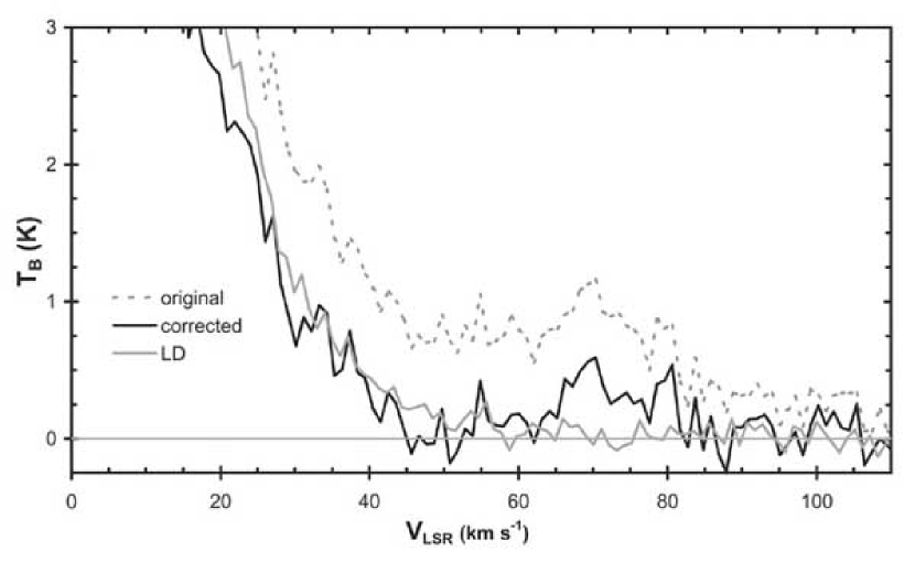
Figure 1: Stray radiation correction. The dashed gray line shows an example of a GBT H I  spectrum (at $9\arcmin$ resolution) observed at $\ell,b=28\fdg 70,20\fdg 35$. The solid gray line is the H I  spectrum from the closest point, of the Leiden-Dwingeloo (LD) $36\arcmin$ resolution H I  survey at $\ell,b=28\fdg 50,20\fdg 50$ (Hartmann & Burton, 1997). The solid black line is the final spectrum, corrected by subtracting from the original GBT spectrum the difference between the GBT data (convolved to match the LD beam) and LD spectrum. The final GBT spectrum shows emission at $V_{\rm LSR}\approx 70$ km s^-1 from a compact cloud which is not detectable in the LD data.

The main problem encountered during data reduction was a contamination of some of the data by stray 21 cm radiation. At certain sidereal times a forward spillover lobe of the GBT admits some Galactic disk emission into spectra taken many degrees away from the plane (see Lockman & Condon (2005)). The stray component produces broad, weak, variable emission on which the real features lie. As a first-order correction for this effect, we renormalized all the contaminated spectra to the Leiden-Dwingeloo (hereafter LD) survey of Hartmann & Burton (1997) in the manner described in Lockman et al. (1986) and Lockman (2002b). The GBT data are convolved to the angular resolution of the LD survey, and any difference between the convolved GBT spectra and that of LD is assumed to be stray radiation in the GBT data, which is then removed from individual GBT spectra. Figure 1 shows a GBT spectrum (at $9\arcmin$ resolution) before and after this correction, and the LD spectrum in the same direction. The GBT spectrum has a line from a compact H I  cloud which is not detectable in the larger ($36\arcmin$) LD beam.

The stray radiation correction procedure sometimes created long, narrow horizontal and vertical artifacts at the boundaries of the survey sections. These are quite noticeable in some of the figures but are essentially small zero-offsets with negligible effect on the analysis. Work is underway to better estimate the stray radiation correction and remove these artifacts. The H I  features we discuss here are discrete in space and velocity and can easily be distinguished from the broad stray H I  component. All measurements reported in this paper have been checked for consistency with the uncorrected data.

3.2 Error Estimates

The rms noise of spectra in the final data cube is typically 0.25 K for the 2 sec. survey regions, and as low as 0.15 K in the deeper areas that have 7 sec. integration times. The error introduced into the total column density, $N_{\mathrm{H\,I}}\,$, by baseline uncertainties is comparable with the error from noise. The stray radiation correction also introduces an error in column density measurements which is difficult to quantify. In this paper we focus on H I  emission features which are discrete in position and velocity, so the uncertainty in $N_{\mathrm{H\,I}}\,$introduced by the stray radiation correction should be comparable to that of noise and the instrumental baseline. In all, the error in $N_{\mathrm{H\,I}}\,$for the features discussed here is $\approx 3\times 10^{18}$ cm^-2 ($1\sigma$) in a single pixel, and about half of this is uncorrelated from pixel to pixel.

4 THE OPHIUCHUS SUPERBUBBLE: OBSERVED PROPERTIES

4.1 A Neutral Hydrogen Plume

Figure 2 is an H I  column density map covering more than 300 square degrees derived from GBT spectra integrated over $60\leq V_{\rm LSR}\leq 100$ km s${}^{-1}\>$. This range of velocities corresponds to gas rotating with the Galaxy near the tangent points at these longitudes, implying a distance from the Sun $r=R_{0}\sin\ell$ if the rotation is purely circular, where $R_{0}\equiv 8.5$ kpc is the distance from the Sun to the Galactic center. The figure shows an object which we call “the Plume,” centered at $\ell,b=30\arcdeg+26\arcdeg$. If it is at the tangent point, it has a distance from the plane $z=3.4$ kpc. It is an irregular structure approximately $10\arcdeg$ by $5\arcdeg$ in size with localized H I  column densities of 2 – 4 $\times 10^{19}$ cm${}^{-2}\>$. There are a few nearby H I  clouds which seem to be related to the Plume, but its main section does not seem to be a group of clouds but rather a singular, albeit complex, object.

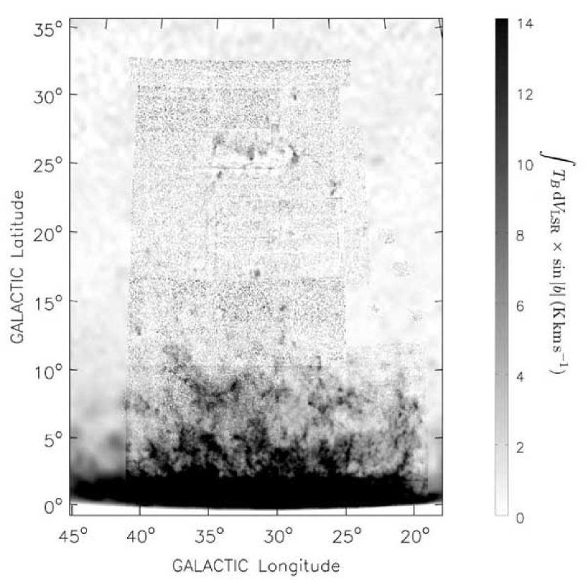
Figure 3: The Ophiuchus superbubble in H I  . Spectra integrated over $60\leq V_{\rm LSR}\leq 160$ km s${}^{-1}\>$ show the Plume in the larger context of the Galactic disk and lower halo. The integration covers all the tangent point velocities at these longitudes. GBT H I  spectra are used for most of the map, but data from the lower resolution Leiden-Dwingeloo survey are used around the edges. The intensity scale has been multiplied by $\sin|b|$ to compress the dynamic range and show structures more clearly. Several coherent H I  features (we dub them “whiskers”) stretch from the disk to $b\geq 15\arcdeg$ ($z\approx 2$ kpc). Dozens of compact but relatively dense clouds fill the space between the whiskers and the Plume. The Plume itself appears to be a cap on top of an unusually violent eruption of gas from the Galactic disk.

Figure 3 shows the entire region of our survey, and the Plume in the larger context of the Galactic disk and lower halo. Here the H I  spectra were integrated over 60 – 160 km s${}^{-1}\>$, a range which covers the tangent point velocities at all these longitudes. Most of the area of Fig. 3 was observed with the GBT, but lower angular resolution data from the LD survey have been added around the edges of the image. Values of $N_{\rm HI}$ vary by several orders of magnitude from low to high latitudes over this region, so as an aid to visualization the data were scaled by $\sin|b|$.

The GBT data show what looks like a system of many filamentary structures (we dub them “whiskers”) reaching from the disk to $b\geq 15\arcdeg$ ($z\approx 2$ kpc). A population of dozens of compact clouds fills the space between the whiskers and the Plume, suggesting that the Plume itself at $b=25\arcdeg$ may be a coherent cap on top of an unusually violent eruption of gas from the Galactic disk. Based on our inspection of the LD and WHAM survey data (the latter is described in §4.2), this system is one-sided and does not extend below the Galactic plane.

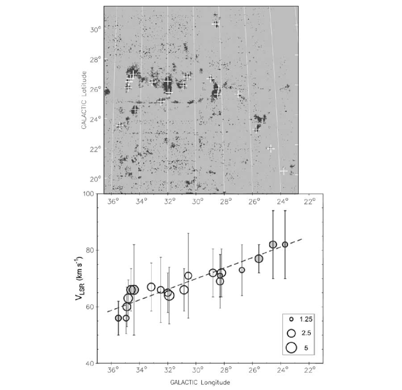
Figure 4: Kinematics of the Plume in relation to its spatial structure. The lower part of the figure shows the velocity of all of the clearly discernable features of the Plume (marked by crosses in the upper panel). The area of each circle is proportional to $\log(N_{\mathrm{H\,I}})\,-19$, where $N_{\mathrm{H\,I}}\,$is the column density in cm${}^{-2}\>$; the legend shows circle sizes for a few values of $N_{\mathrm{H\,I}}\,$in units of $10^{19}$ cm${}^{-2}\>$. The bar through each point shows the FWHM of the line. Measurements made above or below the main section of the Plume at $25\arcdeg<b<28\arcdeg$ are filled with gray and have bolder bars, and show that the coherence of the structure extends even to outlying clouds. The dashed line is a linear fit to the CO terminal velocity measurements in the Galactic plane (Clemens, 1985) with an offset discussed in $\S 5.5$. It shows that the linear dependence of LSR velocity with longitude is fully explained by Galactic rotation and projection effects.

The kinematics of the Plume is shown in relation to its spatial structure in Figure 4. The lower part of the figure shows velocity as a function of the Galactic longitude for the brightest H I  peaks. Only a few clouds with velocities significantly larger or smaller than the rest were excluded from this Figure. We will return to them when discussing the kinematics of the system and its surroundings. Vertical bars on each point indicate the FWHM of the line. The upper part of the figure relates each measurement to its position on the sky. The measurements above or below the strip of $25\arcdeg<b<28\arcdeg$ are filled with gray and have bolder bars in order to distinguish them from the measurements made in the main section of the object.

There is a clear linear dependence of the LSR velocity of the Plume with longitude, a relationship which extends even to the outlying clouds. The slope of $V_{\rm LSR}(\ell)$ matches the slope of the ¹²CO terminal velocities in the Galactic plane (Clemens, 1985) shown by the dashed line. We will see that this is fully explained by the effect of projection of Galactic rotation for an object near the tangent point and is an indication that we are in fact dealing with a single coherent object. The typical FWHM of the lines is about 15 – 20 km s${}^{-1}\>$, which is broader than other known halo clouds (Lockman, 2002a; Lockman & Pidopryhora, 2005), suggesting that the Plume is highly turbulent.

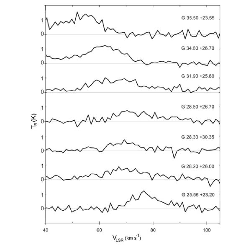
Figure 5: Examples of GBT H I  spectra taken at seven locations within and near the Plume. The typical emission FWHM is 15 – 20 km s${}^{-1}\>$, which is broader than usual for halo clouds, suggesting high turbulence. Unusually wide wings imply a double Gaussian or even more complex line structure. The cloud at G28.30+30.35 lies considerably above the main body of the Plume, but its spectrum is similar to the others.

Examples of spectra taken at seven locations within and around the Plume are shown in Figure 5. Although these are the brightest lines of the system, only a few reach $T_{B}$ $>$ 1 K. Often the lines are not single Gaussians but have a double or even more complex line structure. The spectrum at G28.30+30.35 is from the highest latitude cloud we have detected – well separated from the main body of the Plume but certainly part of it.

4.2 Ionized Hydrogen

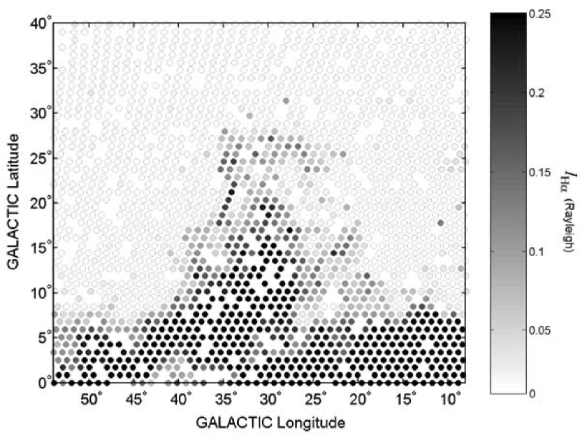
Figure 6: Region of the superbubble in H$\,\alpha\>$, integrated over 55 – 95 km s${}^{-1}\>$LSR, as observed with the Wisconsin H-Alpha Mapper (WHAM; Haffner et al. (2003)). The figure conveys the nature of the WHAM survey. Each circle is centered at the coordinates of a WHAM observation, but for clarity is only half the diameter of the $1\arcdeg$ WHAM beam. The superbubble is a major feature in H${}^{+}\>$as well as H I  , but unlike the neutral hydrogen, the ionized hydrogen fills the area and is not concentrated at its edges. Empty spots occur where bright foreground stars contaminate the data.

The region of our study has been observed in the H$\,\alpha\>$ line of ionized hydrogen with the Wisconsin H-Alpha Mapper (WHAM; Haffner et al. (2003)). Over most of the area the optical extinction is low, and H$\,\alpha\>$ has been detected to a great distance from the Sun (see also Madsen & Reynolds (2005)). Figure 6 shows the H$\,\alpha\>$emission integrated over $55\leq V_{\rm LSR}\leq 95$ km s${}^{-1}\>$, similar to the velocity range used in Figures 2 and 3. The lower velocity limit was chosen as optimal for avoiding the contamination from unrelated emission, while the upper velocity is the limit of reliable data in the WHAM survey.

The Ophiuchus superbubble is clearly a major feature in H$\,\alpha\>$as well as in H I  . However, unlike the H I  , which seems concentrated in the Plume and several “whiskers” marking the edges of the system, the H$\,\alpha\>$is not limb-brightened, and if anything, is brightest in the center of the system. We estimate that any central cavity in the ionized gas is likely to have a radius less than half that of the system: the H${}^{+}\>$is distributed over a large volume rather than in a thin shell.

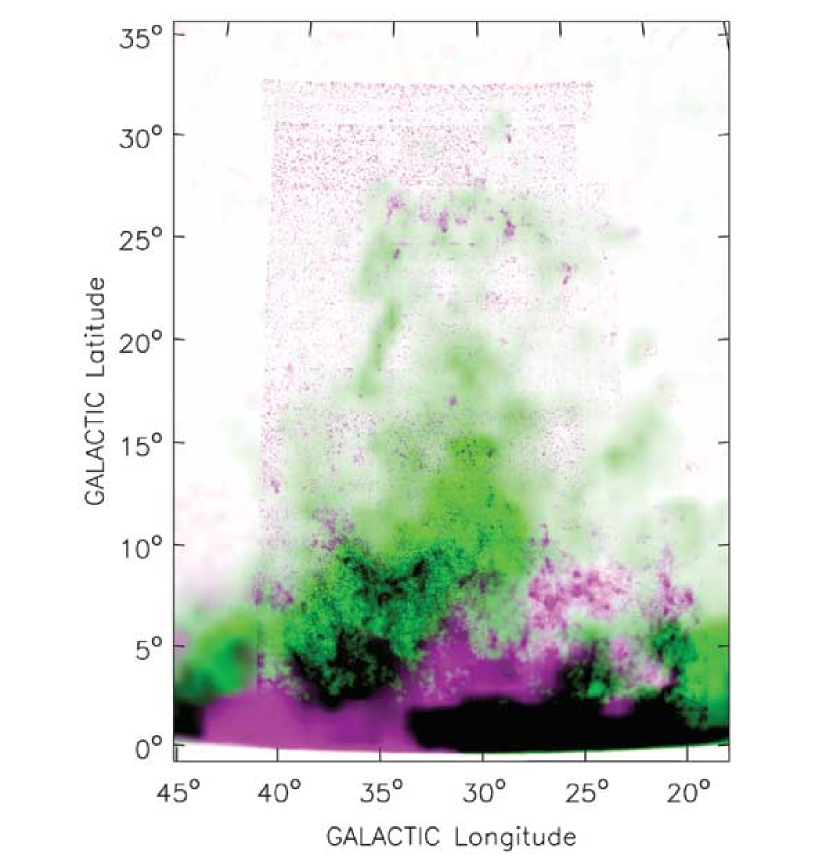
Figure 7: H I  data from Figure 3 (purple) and interpolated H$\,\alpha\>$data from Figure 6 (green). The diagonal purple stripe at the bottom results from extinction of the H$\,\alpha\>$by dust in the Great Rift. There is detailed correspondence between H I  and H$\,\alpha\>$for many features, e. g., the tips of the H I  whiskers at $\ell,b\approx 40\arcdeg+15\arcdeg$ and $30\arcdeg+15\arcdeg$, clouds at $29\arcdeg+31\arcdeg$ and $22\arcdeg+25\arcdeg$, and indeed, the Plume itself. The ionized components of some of the smaller clouds appear shifted to higher longitude than the H I  , but this is probably the effect of the sparsity of the H$\,\alpha\>$survey and its $1\arcdeg$ beam size. The H$\,\alpha\>$emission connects the cap continuously to the Galactic disk and thus suggests that this system is a singular phenomenon of gigantic proportions.

The H$\,\alpha\>$data overlaid with H I  are shown in Figure 7. Green color represents H$\,\alpha\>$and purple H I  . The diagonal purple stripe at the bottom is due to dust in the “Great Rift” attenuating the H$\,\alpha\>$. It is easy to see the correspondence of many features, e. g., the tips of the H I  whiskers at $(\ell,b)\approx(40\arcdeg,15\arcdeg)$ and $(30\arcdeg,15\arcdeg)$, clouds at $(29\arcdeg,31\arcdeg)$ and $(22\arcdeg,25\arcdeg)$, etc., but the most spectacular is the match of the H I  Plume with the top of the ionized hydrogen structure. The H$\,\alpha\>$image of some of the smaller clouds seems shifted to a higher longitude than the H I  , but this is likely the effect of the $1\arcdeg$ beam size of the WHAM and the incomplete sampling of the H$\,\alpha\>$survey. Many clouds are represented by only one or two pixels in H$\,\alpha\>$(Figure 6) and much of the emission is at the limit of the WHAM survey sensitivity. Additional H$\,\alpha\>$ observations of this system are now being made.

The H$\,\alpha\>$shows the continuity between the H I  features near the plane and the high-$z$ parts of the system. H$\,\alpha\>$emission associated with the largest H I  whisker continues upward and appears to connect with the H I  Plume. This correspondence is the primary evidence that at least some of the H I  whiskers are related to the Plume. We conclude that we are seeing a single system of neutral and ionized gas, with H$\,\alpha\>$ emission filling the $\approx 10\arcdeg$ void between the H I  whiskers and the Plume. This system is most probably a coherent structure of gigantic proportions.

4.3 Other Species

At the moment there is no conclusive evidence that the superbubble has been detected in anything other than H I  and H$\,\alpha\>$. There is considerable structure in the soft X-ray emission as measured by ROSAT in this region (Snowden et al., 1997) but most of it appears to arise from absorption in the same dusty foreground medium that blocks the H$\,\alpha\>$. Nothing similar to the H I  or H$\,\alpha\>$  features of the superbubble is found. This is not surprising if we are dealing with a superbubble: its interior is expected to be too hot to be detected in soft X-rays (Veilleux et al., 2005).

There is also no significant correlation with the radio continuum at 408 MHz (Haslam et al., 1982), which closely matches the diffuse soft X-rays in this region. In fact, what we see in both the radio continuum and the X-ray is the tip of the North Polar Spur overlaid on the superbubble. This is probably a coincidence as we can find no detailed correspondence between the H I  and radio or X-ray emission. Also, the North Polar Spur is thought to be a local object at a distance of a few hundred pc (Bingham, 1967; Willingale et al., 2003) while we believe that the superbubble is about 7 kpc away ($\S 5.1$).

Detection of UV metal resonance lines at the velocity of the superbubble would be very useful in uncovering the origins of its gas, but to the best of our knowledge no line of sight in a relevant direction has ever been observed in a UV or optical absorption line.

5 THE OPHIUCHUS SUPERBUBBLE: DERIVED PROPERTIES

5.1 Distance

The H I  velocities of the superbubble, especially the part of it near the Galactic disk, are very close to the tangent point velocities at the corresponding longitudes (see §5.3) and thus we adopt the tangent point distance. For a Sun-center distance $R_{0}=8.5$ kpc and a nominal longitude of $\ell=30\arcdeg$, the tangent-point distance at the base is 7.4 kpc, while if the Plume lies directly above that location, at $b=25\arcdeg$, it must be at a distance of 8.1 kpc.

$V_{\rm LSR}$ changes slowly as a function of distance in the vicinity of a tangent point and thus kinematic distance estimates are not very precise even in the absence of non-circular motions. We adopt a nominal distance of 7 kpc for every part of the system and use a scaling parameter, $d_{7}=d/7$ kpc to show how derived quantities depend on the adopted distance. For a distance to the base of 7 kpc, the Plume, the cap on the superbubble, is at $z=3.4$ kpc from the Galactic plane.

5.2 Size and Mass

The Plume is $10\arcdeg$ in longitude and $5\arcdeg$ in latitude, which corresponds to $1.2\times 0.6$ kpc at a distance of 7 kpc. It has several concentrations with typical diameters of about $100$ pc. To estimate its mass we integrated the column density over the range of 55 to 100 km s${}^{-1}\>$, which is a slightly larger velocity range than is covered in Figure 2, but which includes most of the emission. The total derived H I  mass is $3\times 10^{4}d_{7}^{2}M_{\sun}$, and the H I  mass of an individual clump is about 500 – 1000 $d_{7}^{2}M_{\sun}$.

This mass estimate is subject to a number of uncertainties. It does not include the lower velocity wings of a few high longitude clouds and it unavoidably includes some unrelated H I  from the wings of a few low and high-velocity sources. The former effect is marginal but the latter one might add to the measured mass. By choosing different velocity ranges and sky boundaries, and measuring the mass before the stray radiation correction, we have examined how all these factors change the estimated H I  mass. Alternate choices of velocity range have the most influence on the result and lead to variations in mass of as much as a factor of 2. From a similar analysis we derive masses of a few $10^{5}d_{7}^{2}M_{\sun}$ for each whisker, but here there is an additional uncertainty because whiskers blend with unrelated emission at low latitudes. The estimated mass is thus for that part of a whisker which lies at $b\gtrsim 4\arcdeg$. In our best estimate, the total H I  mass of the superbubble system, evaluated as the sum of the whiskers’ masses and the mass of the Plume, is $\sim 10^{6}d_{7}^{2}M_{\sun}$.

5.3 Kinematics

Because of the large size of the superbubble, projection effects must be considered in analyzing its kinematics. Thus we introduce a new velocity coordinate, the “deprojected” velocity $\upsilon$. For a point of the observed 3D space $(\ell,b,V_{\rm LSR})$,

$$\upsilon(\ell,b,V_{\rm LSR})\equiv V_{\rm LSR}\,\sec(b)-V_{t}(\ell).$$ (1)

Here $V_{t}(\ell)$ is the tangent point velocity for the given Galactic longitude derived from the empirical polynomial relation of Clemens (1985), neglecting his proposed change to the LSR, and $V_{\rm LSR}\sec(b)$ is the measured velocity of an H I   line corrected for the projection of circular Galactic rotation with latitude. Objects in circular rotation near the tangent point will all have a similar value of $|\upsilon|\sim 0$ regardless of their latitude. This deprojection is useful mainly in displaying and visualizing the relationship between objects at different locations; it is less useful for quantitative analysis.

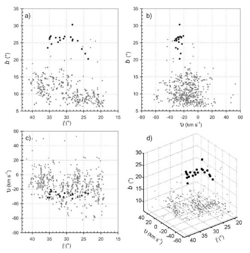
Figure 8: The superbubble system kinematics in $(\ell,b,\upsilon)$ space, where $\upsilon(\ell,b,V_{\rm LSR})\equiv V_{\rm LSR}\sec(b)-V_{t}(\ell)$ is the “deprojected velocity.” Objects in circular Galactic rotation at the tangent point should all have a similar $|\upsilon|\approx 0$. Larger filled points mark measurements on the Plume itself, the same set shown in Figure 4. Panels a) through c) show three 2D projections and panel d) a 3D plot of the same data. The Plume is kinematically compact compared to other parts of the system and has a slight velocity offset.

We identified 636 H I  features which appear to be discrete clouds in the system and measured their central velocities. Such measurements have been performed everywhere it was possible above $b=6\arcdeg$. Closer to the Galactic plane the features are too blended to be distinguished. Resultant values of $\upsilon$ are shown in the four panels of Figure 8. The twenty points belonging to the Plume are marked by a larger size and darker shade. They are the same positions plotted in Figure 4. The kinematic coherence of the Plume stands out. Much of the systematic variations in $V_{\rm LSR}(\ell)$ noted in Fig. 4 arise because of the projection effects. The variation is removed in the deprojection (Fig. 8b). The Plume is seen to be a distinct, coherent structure with kinematics similar to that of the gas in the disk below it, but at a velocity somewhat lower than $V_{t}$. The connection is explored further in $\S$ 5.5.

5.4 Connection to Gas Nearer the Plane

The lower part of the superbubble system shown in Figure 3 consists of whiskers of H I   extending as much as 2 kpc into the Galactic halo. The typical H I  mass of each whisker is a few $10^{5}\ d_{7}^{2}\ M_{\sun}$. The H$\,\alpha\>$data clearly show that the superbubble has continuity from its H I  cap, the Plume, down to the plane, but the existing H$\,\alpha\>$data provide little kinematic information on the connection.

In Fig. 8b we see some H I  features which lie spatially and kinematically between the Plume and the bulk of the emission at lower latitude, but their connection with the superbubble, if any, cannot be established from existing data. Clouds that lie at some significant distance from the tangent point have values of $\upsilon\ll 0$. As seen in the figure there are many such objects within the analyzed set of measurements. They are probably unrelated to the superbubble.

We conclude that there is a clear connection between H I  in the disk and that in the Plume, but the kinematic structure of the entire system remains uncertain.

5.5 Plume Kinematics: Corotation or Lag?

An object far from the Galactic plane, like the Plume, may not be corotating with the material below it. In fact, it is expected to lag significantly behind Galactic rotation, i.e., $V_{\theta}(z=3\ \mathrm{kpc})<V_{\theta}(z=0)$, and it may have a vertical velocity, $V_{z}$, as well (Collins et al., 2002). We test this possibility for the Plume atop the superbubble. As the reference for normal Galactic rotation we use the molecular clouds which lie close to the plane and have a small component of random motion; their kinematics can be traced in spectral lines such as ¹²CO.

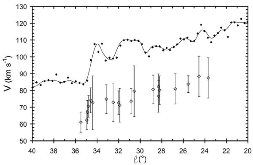
Figure 9: Velocity of the Plume components compared to that of molecular clouds at the tangent point. The filled points are measurements of the ¹²CO terminal velocity in the Galactic plane (Clemens, 1985). The curve is a cubic spline interpolation fit to the median filtered ¹²CO velocities. The open symbols show the Plume’s H I  velocity, $V_{\rm LSR}\,\sec(b)$, and the vertical bars show the line FWHM. The Plume traces the kinematics of the molecular gas, but with an offset velocity.

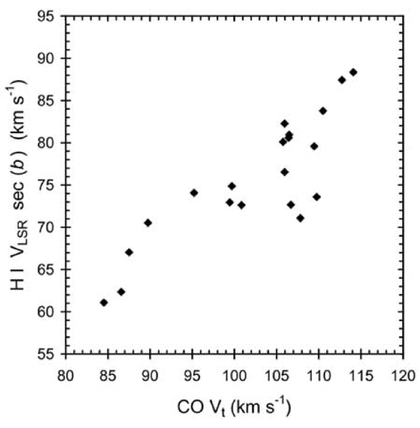
Figure 10: Velocities of Plume H I  features shown in Figs. 4, 8 and 9, $V_{\rm LSR}\,\sec(b)$, plotted versus the ¹²CO terminal velocity at the same longitude in the plane. The Pearson correlation coefficient of the two sets is 85.3%. Despite its location at $b\approx 26\arcdeg$ ($z>3$ kpc), the Plume still bears a detailed imprint of the rotation of the Galactic disk.

Figure 9 shows measurements of the tangent-point velocity, $V_{t}$, of ¹²CO in the Galactic plane over the longitude range of the superbubble (Clemens, 1985) that have been fit with a spline curve which captures the small-scale structure. For this fit the ¹²CO measurements were filtered with a $1\arcdeg$ median filter, and evaluated every $30\arcmin$. The terminal velocity of ¹²CO changes by $>30$ km s${}^{-1}\>$over this region. The sharp jump at $\ell\approx 35\arcdeg$ is seen in low-latitude H I  as well as CO (Burton & Gordon, 1978), and may be related to density wave streaming, though it is not a feature of recent models (Bissantz et al., 2003). The points below the CO curve show the LSR velocity of the Plume corrected for projection of circular rotation, $V_{\rm LSR}\,\sec(b)$, and the vertical bars show the FWHM of the H I  lines. The CO and H I  track each other with a nearly constant offset. The correlation between velocities in the plane and in the superbubble cap is shown further in Figure 10. They are correlated at the 85.3 percent probability level (Pearson correlation coefficient).

For an object near the tangent point, the velocity components expressed in galactocentric coordinates $(R,\theta,z)$ project to the LSR in the following way:

$$V_{\rm LSR}=R_{0}\sin(\ell)\cos(b)\left(\frac{V_{\theta}}{R}-\frac{V_{0}}{R_{0}}\right)+V_{z}\sin(b)$$ (2)

where $V_{\theta}$ and $V_{0}$ are the azimuthal (rotational) velocities at $R$ and at the Sun, respectively, and $V_{z}$ is a vertical component of motion, taken to be positive in the direction of the north Galactic pole. Near the tangent point, velocities which are radial with respect to the Galactic center, $V_{R}$, project across the line of sight and do not enter into $V_{\rm LSR}$.

For an object at the tangent point, where $R=R_{0}\sin(\ell)$, we can write

$$V_{\rm LSR}=V_{\theta}-V_{0}\,\left(\frac{R}{R_{0}}\right)\equiv V_{t},$$ (3)

and define a lag velocity

$$V_{lag}(z)=V_{\theta}(z)-V_{\theta}(0).$$ (4)

which quantifies the difference between the rotational velocity in the halo and that in the plane. Rewriting equation 2 for an object at the tangent point:

$$V_{\rm LSR}=(V_{t}-V_{lag})\cos(b)+V_{z}\sin(b).$$ (5)

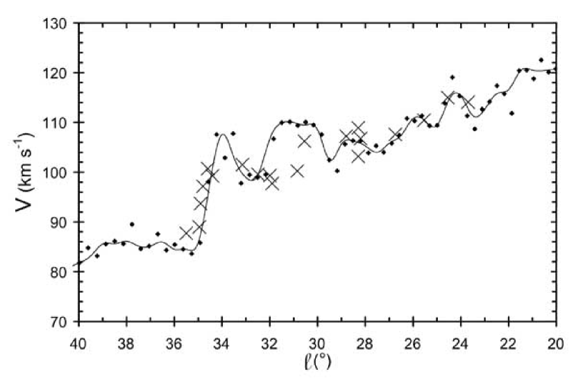
Figure 11: Velocity structure of the Plume, compensated for lag, compared with that of molecular gas at the tangent point. These are the same data as in Fig. 9, but with the H I  velocities (marked here with crosses) increased by 26.6 km s${}^{-1}\>$. The close agreement of these measurements shows that the Plume at $z>3$ kpc shares the same kinematics as molecular clouds in the Galactic plane, even in considerable detail. Its kinematics are thus dominated by Galactic rotation.

We have fit this equation to the H I  in the Plume using, for $V_{t}$, the spline curve from the ¹²CO data of Figure 9. The solution with $V_{z}\neq 0$ fails the F-test with certainty very close to 100%, i.e., we can detect no significant vertical motion of the Plume within the statistical error of 22 km s${}^{-1}\>$. Interpreting the difference between the Plume and CO velocities as arising from a lag in rotational velocity, we find $V_{lag}=26.6\pm 4.6$ km s${}^{-1}\>$($1\sigma$). The H I  data corrected for the derived lag are shown in Figure 11. The velocities of the H I   Plume atop the superbubble match ¹²CO terminal velocities in the plane extremely well, in some cases even following fine structure in $V_{t}$. This is strong evidence that the motion of the Plume is determined by the gravitational field of the Galaxy, and not local conditions.

There is, however, another possible interpretation of the velocity difference between the Plume and the tangent point: the superbubble system may not be located at the tangent point. If we interpret the Plume’s velocity using a model requiring cylindrical Galactic rotation for all heights above the disk, i.e., $V_{\theta}(z)=V_{\theta}(0)$, its implied location is either at a “near” distance of 5 kpc (and $z=2.4$ kpc) or a “far” distance of 11 kpc with $z=5.4$ kpc. In this case, however, the H I  whiskers rising up from the plane very close to the tangent point must not be related to the Plume despite the fact that H$\,\alpha\>$ emission connects all parts of the system. This alternate interpretation still leaves the Plume extremely far from the Galactic plane, where some lag from corotation is expected anyway.

We conclude that it is most likely that: 1) The superbubble is a coherent system whose kinematics derive primarily from Galactic rotation; 2) The distance to the system is approximately the tangent point distance, 7 kpc; 3) the kinematics of its cap, the Plume, are consistent with a lag in Galactic rotation of $26.6\,\pm\,4.6$ km s${}^{-1}\>$at a location $R=4$ kpc and $z=3.4$ kpc; 4) The Plume shows no significant evidence for vertical motions.

5.6 Potential Energy

As a lower limit on the energy needed to produce the superbubble, we can estimate the gravitational potential energy of the Plume. Let us assume that initially the mass now in the cap was at rest in the Galactic plane, rotating with the Galaxy. Then, using a Galactic potential model, we can estimate the energy required for it to reach its current position. Both the graphs in Collins et al. (2002) (derived from the potential by Wolfire et al. (1995)) and calculations with the GalPot package by Walter Dehnen (Dehnen & Binney, 1998) give the same result: an object in the plane at $R=4$ kpc would have to be given a vertical velocity of $\approx 200$ km s${}^{-1}\>$to reach $z=3.4$ kpc. Combined with our estimate for the Plume’s H I  mass this gives:

$$E_{pot}>10^{52}\;d_{7}^{3}\;\mathrm{erg}.$$ (6)

An exact calculation with the GalPot package gives the identical result of $1.8\times 10^{52}\;\mathrm{erg}$.

5.7 Ionization

The H$\,\alpha\>$data can be used to derive the rate of emission of ionizing photons illuminating the Plume from the Galactic plane. For this purpose we use a small cloud separated from the main body of the Plume, though clearly associated with it: the cloud at $\ell\approx 29\arcdeg$, $b\approx 31\arcdeg$, whose angular size is approximately $1\arcdeg$ in H I  .

The GBT spectra show that this cloud has a foreground $N_{\mathrm{H\,I}}\,$$=6\times 10^{20}$ cm^-2, implying a visual extinction $A_{V}=0.3$ mag for a standard dust-to-gas ratio (Diplas & Savage, 1994). We neglect this modest extinction in this initial analysis of the ionized gas, where we seek only to understand the general nature of the system. Subsequent studies will take this into account, however, for it becomes increasingly important at lower latitudes.

The total H$\,\alpha\>$intensity of this cloud in the WHAM survey is $I_{\alpha}\approx 0.1$ Rayleigh, which corresponds to a production rate of $10^{5}$ H$\,\alpha\>$photons cm^-2 s^-1. For Case B recombination this requires ionization by a Lyman continuum photon flux

$$F_{\rm LC}=2\times 10^{5}\left(I_{\alpha}\over{0.1{\rm R}}\right){\rm ph\ s^{-1}}$$ (7)

(Tufte et al., 1998). Neglecting geometric factors, and assuming that the photon source is a point located a distance $z$ from the cloud, the source production rate of Lyman-continuum photons is

$$Q(LC)\approx 2\times 10^{6}\,I_{\alpha}\cdot 4\pi z^{2}.$$ (8)

For the cloud at $29\arcdeg+31\arcdeg$ with $z=7\ \tan(31\arcdeg)=4.2$ kpc,

$$Q(LC)\approx 5\times 10^{50}d_{7}^{2}\;\mathrm{ph}\;\mathrm{s}^{-1}.$$ (9)

This value is consistent with the output of 100 typical O-class stars (Martins et al., 2005).

The Ophiucus superbubble lies near many H II regions and young stellar clusters, though its size is so large that we cannot pinpoint a singular source of its ionization. The W43 cluster at $\ell\approx 30\arcdeg$ generates $10^{51}$ Lyman-continuum photons s^-1 (Smith et al., 1978), enough to ionize the Plume if the path between the two is unobscured. This is discussed further in $\S 7$.

5.8 H${}^{+}\>$Mass of the Superbubble

Assuming that the temperature of the H${}^{+}\>$is 8000 K, a typical value for the Galactic ionized medium (Reynolds, 1985), each Rayleigh of H$\,\alpha\>$ emission corresponds to an emission measure of 2.25 cm^-6 pc (Haffner et al., 1998). The superbubble is about 2 kpc wide and we assume the same value for the emission depth $l_{EM}$ (which is also subject to the distance uncertainty factor $d_{7}$). The average electron density inside the structure is

$$\bar{n}_{e}\,(\mathrm{cm}^{-3})=\left(\frac{2.25I_{\alpha}(\mathrm{R})}{f\,l_{EM}(\mathrm{pc})\,d_{7}}\right)^{1/2}\,$$ (10)

where $f$ is the filling factor of ionized gas along the line of sight. The lack of strong limb-brightening in H$\,\alpha\>$($\S$4.2) leads us to adopt $f\gtrsim 0.5$. For simplicity we ignore a possible difference between the line-of-sight and volume filling factors. In the superbubble the typical observed $I_{\alpha}=0.2$ R, so, neglecting extinction, $\bar{n}_{e}=0.015\,f^{-1/2}\,d_{7}^{-1/2}$ cm${}^{-3}\>$. The H${}^{+}\>$mass is given by

$$M_{\mathrm{H}^{+}}(M_{\sun})=2.47\times 10^{7}f\,\bar{n}_{e}(\mathrm{cm}^{-3})\,V(\mathrm{kpc}^{3}).$$ (11)

For the 5 – 8 $d_{7}^{3}$ kpc³ volume of the system, the values of $\bar{n}_{e}$, and $f$ give

$$M_{\mathrm{H}^{+}}=1-3\times\,10^{6}\,d_{7}^{2.5}\,M_{\sun},$$ (12)

a mass similar to that in H I  .

5.9 Vertical Density Structure of a Whisker

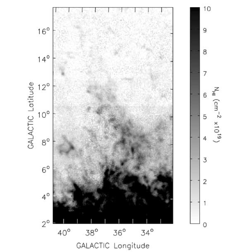
Figure 12: GBT H I  observations of a prominent whisker of H I  which may be the wall of the superbubble. This image is integrated over $70\leq V_{\rm LSR}\leq 90$ km s${}^{-1}\>$, velocities which cover the tangent points in this direction, where $1\arcdeg$ corresponds to 120 pc. The whisker thus extends about 1.5 kpc into the halo.

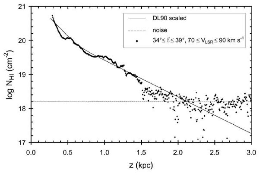
Figure 13: Vertical density structure of the whisker from Fig. 12. The points show $N_{\mathrm{H\,I}}\,$of the H I  whisker averaged over $5\arcdeg$ of longitude, plotted against distance from the plane assuming that the whisker is at the tangent point. The top of the whisker is at $z\approx 1.5$ kpc. The solid curve shows the empirical $N_{\mathrm{H\,I}}\,$$(z)$ derived by Dickey & Lockman (1990) over the inner Galaxy, scaled to a 1.6 kpc path length. The agreement between the curve and points suggests that the vertical structure of the whisker is essentially the vertical structure of the general ISM. The whisker is thus not likely to be material thrust up from the plane, but rather a wall of gas swept up from the side, as would be expected if it is the wall of a superbubble.

The vertical structure of a “whisker” can give insight into its origin. Figure 12 shows the best example of an H I  whisker which is likely to be connected to the superbubble. Here the emission is integrated over $70\leq V_{\rm LSR}\leq 90$ km s${}^{-1}\>$, which covers the tangent point velocities at its longitude. There are a number of similar H I   features in the GBT data. Figure 13 shows the whisker’s $N_{\rm HI}$ averaged over $5\arcdeg$ in longitude. For comparison, the solid curve is the $N_{\mathrm{H\,I}}\,$$(z)$ expected for a 1.6 kpc path through the Dickey-Lockman (DL) empirical H I  layer (Lockman, 1984; Dickey & Lockman, 1990). The DL function was derived from 21 cm measurements covering both sides of the Galactic plane and averaged over $3.5\leq R\leq 7.5$ kpc. It should be representative of the vertical structure of the H I  layer in the inner Galaxy.

We see that the vertical density structure of the whisker resembles that of the average interstellar medium. This would not necessarily be the case if the whisker were a column of gas thrust up from the disk. Indeed, a similar analysis along a cut through the Plume shows it as a clear excess of gas above any scaled DL curve at $z=3.4$ kpc. Thus we have the strong implication that the whisker is gas swept up from the side, e.g., perpendicular to the walls of an expanding bubble. The gas in the Plume has been carried up to its location, but the gas in the whisker has not. If we could separate the whisker from unrelated emission, its effective depth, i.e., the path through the DL layer needed to give its $N_{\mathrm{H\,I}}\,$, would be a measure of the volume swept out to make the whisker. The value of 1.6 kpc for the curve in Figure 13 is consistent with the size of the system, but should not be given much significance at this stage of our understanding. This particular whisker is seen in H$\,\alpha\>$, but is so faint that a more detailed analysis of its ionization is impossible.

H I  “worms”, objects morphologically similar to our whiskers, have been discussed by Heiles (1984) who suggested that they are “probably parts of shells that are open at the top”. This is consistent with our conjecture that whiskers are formed by a sideways motion rather than an upward thrust.

6 A MODEL FOR THE OPHIUCHUS SUPERBUBBLE

It is possible to test the hypothesis that this entire system is a superbubble blown by a cluster of young stars in the disk by comparing our data with a model of a superbubble. We use the idealized analytical Kompaneets 2D model (Kompaneets, 1960) to draw possible bubble boundaries, determine the position of the walls and cap in relation to the parent star cluster, and derive a general estimate of the time and energy scales required in such a scenario. The Kompaneets model has been adopted by Mac Low & McCray (1988), Bisnovatyj-Kogan & Silich (1995) and then by Basu et al. (1999) to describe a superbubble expanding from the disk of the Galaxy into an exponential atmosphere with a scale height $H$. The main virtues of such a simple model are its ease of use and clear representation of the principal physical processes involved. It also has many limitations. It is not as exact as modern 2D and 3D simulations and, as noted by Mac Low et al. (1989) and Koo & McKee (1990), its numerical predictions may be off by up to a factor of 2. It also describes the bubble evolving in complete isolation while in reality its evolution is influenced by many external factors like Galactic gravitational and magnetic fields, perturbation by other bubbles, etc. Nevertheless, the model is a suitable starting point for checking the plausibility of the superbubble hypothesis and its quantitative errors are acceptable given that all the properties of the Ophiuchus system are as yet known only to within a factor of a few.

The model follows the standard paradigm of adiabatically evolving bubbles (Weaver et al., 1977; Mac Low & McCray, 1988). It assumes that the bubble is formed around a cluster of stars with a constant total mechanical luminosity $L_{0}$. Initially the cluster winds expand freely and form a shock driving into the ambient ISM. Almost from the time of the bubble’s formation it can be treated as a very thin and dense shock-shell filled with a rarefied gas. Assuming that the shock front moves normal to itself and that its expansion speed is determined only by the internal pressure $P(t)$, ambient density $\rho(z)$, and the ratio of the specific heats $\gamma$, Kompaneets (1960) found that the shell’s shape at every moment of time is described by a curved surface from the following family:

$$r(z,y)=2H\arccos\left[\frac{1}{2}e^{z/2H}\left(1-\frac{y^{2}}{4H^{2}}+e^{-z/H}\right)\right].$$ (13)

Here $r$ is the radial cylindrical variable: as the density is assumed constant for fixed $z$ the surfaces are axially symmetric. The top and bottom of the curve, where $r=0$, are located at:

$$z_{1,2}=-2H\,\ln\left(1\mp\frac{y}{2H}\right).$$ (14)

The parameter $y$ has dimensions of length and varies from 0 to $2H$. It is a nonlinear function of time, energy and volume of the bubble, but its meaning is best understood from a purely geometrical point of view. It follows from equation 13 that by using $r/2H$, $z/2H$ and $y/2H$ instead of $r$, $z$ and $y$ the equation can be rendered dimensionless. The scale height $H$ then sets the scale of the shell, while its shape is governed solely by the parameter $y$. The dimensionless “evolution factor” $y/2H$ varies from 0 to 1 describing the evolutionary stage of the bubble. A value of zero corresponds to a point at the source at the moment of origin, $t=0$. For $y/2H\lesssim 0.5$ the shape is almost spherical, then for $0.5\lesssim y/2H<1$ it becomes ellipsoid-like, getting more and more elongated in the $z$ direction. Finally, for $y/2H=1$ the bubble’s surface is a paraboloid-like shape stretching up to infinity. Physically this means infinite shock acceleration in the upward direction due to a strong density gradient, the “blowout” scenario, when the bubble’s top is completely disrupted and the bubble becomes a “chimney”.

Another possibility is the “stall” scenario. For values of $y\approx 2H$ the strong shock approximation is no longer valid and thus the Kompaneets model becomes unphysical. The shell expansion stalls when its speed falls to the sound speed of the external medium, which is the same moment when the pressure in and out of the bubble equalizes. By then the walls and the cap of the bubble begin to decompose and finally the shell merges with the surrounding ISM.

Ideally, to allow for the development of a one-sided bubble its origin must be somewhat above the Galactic plane. In reality, even if this condition is not satisfied the development of the downward lobe can be blocked by a dense molecular cloud or some other density fluctuation common in the Galactic plane, especially in a spiral arm where the bubble’s parent star cluster was likely located.

Within the Kompaneets framework, the age and internal thermal energy of the bubble, $E_{th}$, (which is just the mechanical energy from the source cluster, $L_{0}t$, minus the work done on the shell expansion) is obtained by solving the equations numerically to get $y$ explicitly through time. However, Basu et al. (1999), who performed this numerical evaluation, found that the solutions for time and energy closely follow those for the much simpler spherically symmetric model of Castor et al. (1975) if their shell radius $R_{s}$ is made equal to $y$. Thus we can use the following approximate formulae for the age of the bubble and its internal energy (Castor et al., 1975; Basu et al., 1999):

$$t \simeq \left(\frac{154\pi}{125}\right)^{1/3}\>y^{5/3}\>\rho_{0}^{1/3}\>L_{0}^{-1/3},$$ (15)

$$E_{th} \simeq \frac{5}{11}\>L_{0}\,t.$$ (16)

Note that when the shell has evolved to its maximum diameter the Kompaneets energy is less than the one calculated from the spherical model.

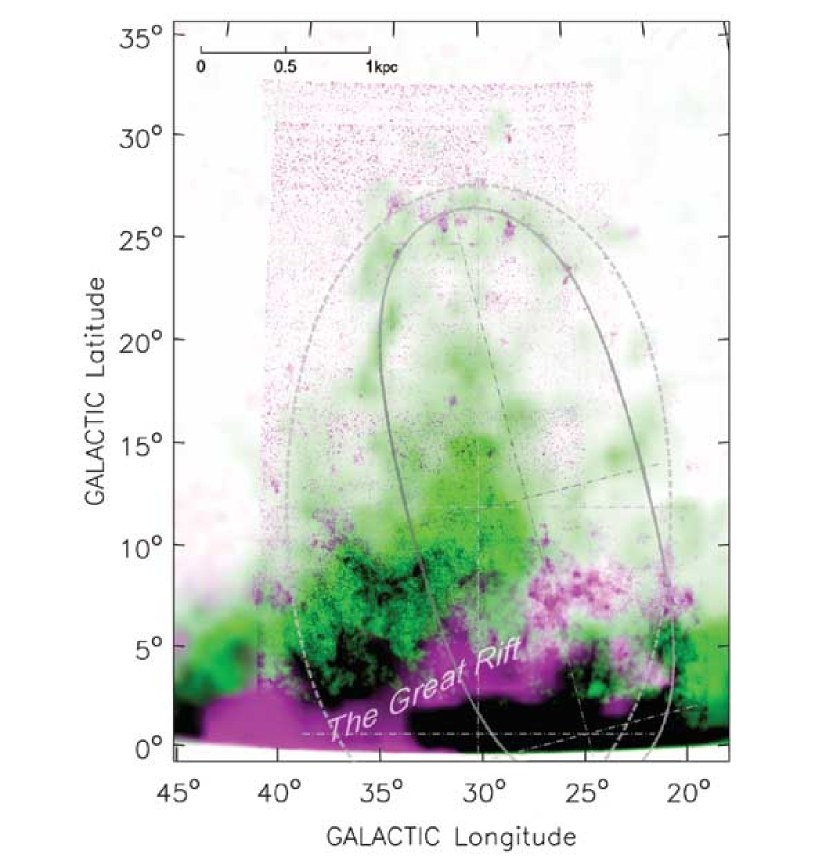
Figure 14: H I  and H$\,\alpha\>$images of the Ophiuchus superbubble (from Fig. 7) with two Kompaneets models that might describe its structure. They share the same latitude of origin slightly above the plane, but differ in aspect ratio and tilt. A distance scale is given at the top of the Figure. The implied ages and energetics of the two models are quite similar, and, because the system is so large, are reasonably robust to small changes in initial conditions. A tilt is expected from the change in gravitational potential over so large a system, and matches the general tilt of the H I  whiskers.

In Figure 14 two Kompaneets curves are plotted on the combined H I  and H$\,\alpha\>$data from Figure 7. We have assumed a constant distance scale (shown in the upper left corner) for the entire figure based on the distance to the system of 7 kpc. Both models have their center of origin at the same $z$, close to the Galactic plane. The model parameters are given in Table 1.

The solid curve (Model 1) was fit by hand to the brightest H I  whiskers and clouds, and goes through the dense H$\,\alpha\>$region at $\ell\approx 35\arcdeg$ , $15\arcdeg\lesssim b\lesssim 25\arcdeg$. In order to do this the curve had to be tilted by $14.5\arcdeg$ in the outward direction relative to the Galactic center. This tilt is consistent with the behavior of the whiskers, which are all tilted by $10\arcdeg-20\arcdeg$ in the same direction. It is also consistent with the effect of the Galactic gravitational potential which the Kompaneets model does not take into account at all: any object thrown vertically from the Galactic plane at $\ell\sim 30\arcdeg$ will drift to a higher longitude while it moves upward. The results of throwing an object to reach $z$ of a few kpc would give us the same effective outward tilt angles of $10\arcdeg-20\arcdeg$ (Collins et al. (2002), and calculations from GalPot (Dehnen & Binney, 1998)). Model 1 also has a benefit of being narrow, and because of that does not extend significantly into and below the Galactic plane.

A wider Kompaneets model that still reaches the same height from the plane would need either an origin at a higher $z$, or an extent some distance below the Galactic plane where, in a realistic situation, it would create a second lobe extending into the halo below the disk. We do not observe a second lobe, but created Model 2 (the dashed curve) mainly to test the generality of the results derived from Model 1. Model 2 is not tilted and was manually fit to contain most of H I  and H$\,\alpha\>$of the system.

Both models have an evolution factor, $y/2H$, almost equal to unity. It is interesting that the atmospheric scale height needed to match the shape and size of the system is not unreasonable. The position of the cap in relation to the Galactic disk where the bubble’s source is located is consistent with the superbubble hypothesis. These conclusions would hold for any Kompaneets curve fit to the Ophiuchus system because the height of the superbubble is so much larger than its width. The meaning is simple: this bubble is already stalled/blown and is dissipating, or it is approaching the stall/blowout. This is the main qualitative result we get from the Kompaneets model.

We evaluated eqs. 15 and 16 for arbitrary $n_{0}$ and $L_{0}$ and then for a few typical values. A typical young star cluster has a mechanical luminosity of $10^{5}\>L_{\sun}$ (Dove et al., 2000; Smith, 2006) so this is used as a reference value. The central density is chosen to be 1 cm${}^{-3}\>$, though other possibilities were examined to understand the sensitivity of the derived properties to the input density. The results are presented in Table 1. One column shows how the calculations would change depending on the value of the distance to the system. As the bubble is close to the end of its evolution, the age calculation should be treated as a lower limit, while the energy is an upper limit.

The model properties differ by a factor of only 2.5, an insignificant difference in view of its limitations. Any Kompaneets model constrained to have a source near the plane and upper end at the Plume would give similar results. The models give an age of the bubble whose order of magnitude is:

$$t\gtrsim 10\>d_{7}^{5/3}\;\mathrm{Myr},$$ (17)

which can be compared with the ballistic age of the Plume, i. e., the time necessary for it to reach its current position at $z\approx 3\;\mathrm{kpc}$ from a single vertical thrust of velocity applied at the Galactic plane. From the GalPot package this time was found to be $\approx 30\;\mathrm{Myrs}$. It is interesting that this age corresponds to the time of onset of fragmentation of a superbubble shell due to instabilities (Dove et al., 2000). Both Rayleigh-Taylor and gravitational instabilities may appear in the late phases of bubble evolution. When a bubble has expanded to the point that its interior pressure is similar to the exterior pressure, characteristical Rayleigh-Taylor “fingers” will form and break, producing a debris of cold cloudlets (Breitschwerdt & de Avillez, 2006). The shell may also become gravitationally unstable at the same time as well, also resulting in shell fragmentation (Elmegreen & Lada, 1977; McCray & Kafatos, 1987; Voit, 1988). The structure of the Plume suggests that it might be just at this point in its evolution. Based on coincidence of these three different age estimates we conclude that the age of the bubble is most likely to be $\approx 30$ Myr.

The total internal energy of the system has the limit

$$E_{th}\lesssim 10^{53}\>d_{7}^{5/3}\;\mathrm{erg},$$ (18)

which is comparable to the estimate of the gravitational potential energy of the Plume discussed in § 5.6. Combining these two estimates, the total energetics of the system is in the $10^{52-53}\;\mathrm{erg}$ range. Of course, we do not know the nature of the parent stellar cluster, so we cannot tell if it suffers the “energy-deficit problem” observed in other systems (Oey & García-Segura, 2004; Cooper et al., 2004). The Ophiuchus superbubble could have been formed by an OB association containing about 70 O stars, similar to the Carina Nebula, which will contribute to the ISM about $2.6\,\times\,10^{52}$ erg through stellar winds over 3 Myr (Smith, 2006).

7 THE OPHIUCHUS SUPERBUBBLE IN THE GALAXY

The H I  and H$\,\alpha\>$superbubble lies above a section of the Galaxy which contains many sites of active star formation. The H II region and molecular cloud complex W43, at $\ell\approx 30\arcdeg$, near the tangent point of the Scutum spiral arm, has been called a ‘mini-starburst’, where the star formation efficiency has apparently been enhanced over the last $10^{6}$ yr (Motte et al., 2003). The brightest H II region in W43 is G29.944-0.042 with a radio recombination line velocity of 96.7 km s${}^{-1}\>$, and there are many other H II regions within a few degrees that have the $70-100$ km s${}^{-1}\>$velocities of the H I  whiskers and Plume (Lockman, 1989). Although the superbubble has an age $>10$ Myr and was likely produced by a generation of young stars previous to the current W43 cluster, W43 is known to generate at least $10^{51}$ Lyman-continuum photons s^-1 based on the radio observations that trace the absorbed fraction (Smith et al., 1978). The W43 stars clearly have sufficient ionizing luminosity to ionize the superbubble, if the disk medium allows a moderate leakage of Lyman-continuum photons into the halo.

The Plume itself is so far from the plane that it is probably exposed to ionizing radiation from several spiral arms in the inner Galaxy. Because we have a good estimate of its distance, it can act as a probe of the radiation field above the disk. It has an H$\,\alpha\>$flux similar to that of some high-velocity clouds also detected with the WHAM instrument (Tufte et al., 1998, 2002), and the implied Lyman-continuum photon flux needed to maintain its ionization, $2\times 10^{5}$ photons cm^-2 s^-1, is in the range of that expected from models of an object at its location (Bland-Hawthorn & Maloney, 2002; Putman et al., 2003).

8 CONCLUDING DISCUSSION

Using 21 cm H I  spectra measured with the GBT, we have discovered a large coherent structure located in the inner Galaxy at a distance of about 4 kpc from the Galactic center and 7 kpc from the Sun. Its top reaches $>4$ kpc above the Galactic plane and is visible in both ionized and neutral hydrogen emission. The structure of the H I  , the location and intensity of the H$\,\alpha\>$emission, and the analysis of the system’s kinematics, give a consistent picture: most probably we are seeing a superbubble blown by the joint action of stellar winds and multiple supernovae from a star cluster in one of the Galaxy’s spiral arms. The model shows that the energetics required to power the creation of a bubble of this size is of the same order as is produced from a typical OB association. The structure’s age is $\approx 30$ Myr and the OB stars in the cluster, which formed the bubble, have thus already evolved off the main sequence. A different, younger cluster must be the source of ionizing photons which produce the observed H$\,\alpha\>$. A summary of the properties of the H I  cap on the system is given in Table 2, and a summary of the properties of the system as a whole is in Table 3.

The Plume, the neutral cap on top of the system, is very irregular with broad lines suggesting substantial turbulent motions. And yet, its overall kinematics match the kinematics of molecular clouds in the plane below it quite well, with a lag of 27 km s${}^{-1}\>$. Extra-planar gas is expected to show a gradient in rotational velocity arising from a change in the gravity vector with $z$, and recent models have attempted to reproduce the magnitude of the effect observed in other galaxies (Collins et al., 2002; Barnabè et al., 2006; Fraternali & Binney, 2006). In the Milky Way, evidence for deviations from corotation is suggestive but not compelling (Savage et al., 1990, 1997). The Plume stands as the best single example of a Galactic cloud with a significant, and coherent, lag behind corotation.

The Kompaneets model indicates that we are seeing either the late stages of the bubble’s development or the early stages of its decomposition. This is consistent with our failure to detect any significant vertical motion of the Plume. At the age of this system several instabilities should begin to fragment a superbubble shell (Dove et al., 2000). The turbulent, irregular structure of the Plume, with its outlying clouds, may be a sign that this process is already underway. In about 30 Myr (the ballistic free-fall time) all the material will return to the Galactic disk.

The vertical density structure of one of the H I  whiskers found at the base of the system is similar to the average vertical density structure over the inner Galaxy. This is consistent with the hypothesis that this whisker is part of the superbubble’s walls swept by an expansion perpendicular to its surface. Despite its suggestive appearance, we do not believe that this whisker results from an outflow along its axis but rather a sidewise push. Other vertical structures have been identified in Galactic H I  and interpreted as outflows (Heiles, 1984; Koo et al., 1992; English et al., 2000; de Avillez & Mac Low, 2001; Asgekar et al., 2005; Kudoh & Basu, 2004). Although the mass of some of these is in range of the mass of the whiskers in the Ophiuchus superbubble system, they are typically smaller by a factor of ten in size. The whiskers detected here more nearly resemble the vertical dust lanes seen with the WIYN telescope in NGC 891 as pillars of extinction extending to $z\sim 2$ kpc against the light of that galaxy (Howk & Savage, 2000). Like the whisker of Fig. 12, they contain $\sim 10^{5}M_{\sun}$. It is interesting that the linear resolution of the GBT in the 21 cm line of H I  at the Ophiuchus superbubble is essentially identical to that of the WIYN telescope at NGC 891.

This superbubble is very different from an M82-type nuclear starburst (Weiß et al., 1999; Matsushita et al., 2005): the energies and densities involved are orders of magnitude smaller. It can, however, be compared with known bubbles in normal and dwarf galaxies.

An analysis of observations of bubbles and shells both in the Milky Way and other galaxies shows that bubbles fall into two general categories divided by their age. “Young” bubbles have typical sizes of a few hundred pc, expansion velocities of $\gtrsim 20$ km s${}^{-1}\>$and ages of a few Myr. “Old” bubbles have typical sizes of more than 1 kpc, expansion velocities of $\lesssim 10$ km s${}^{-1}\>$and ages of a few tens of Myr. Old supershells usually are not very abundant in normal spiral galaxies, possibly because of the presence of differential rotation, destructive to large coherent structures. However there are still several known in the Milky Way and a few in similar galaxies like M31 and M33 (McClure-Griffiths et al. (2002); Kim et al. (1999); Ehlerová & Palouš (2005); Walter & Brinks (1999) and references therein). In the shell classification scheme of Kim et al. (1999), which is based on the relation between H I  and H$\,\alpha\>$, the Ophiuchus superbubble belongs either to Type I (shell filled with ionized gas) or Type V (discrete H II regions inside the shell due to secondary star formation inside the shell). Type I is a characteristic of young bubbles at the earliest stages of their development so it probably does not apply here, while Type V is consistent with both the old age and a large number of H II regions near the base of the superbubble, and also with the broad distribution of H${}^{+}\>$within the system. New ionization sources develop after the death of the parent cluster not by chance, but as a consequence of the bubble’s evolution.

The Ophiuchus superbubble with its size $\sim 2$ kpc, age of $\approx 30$ Myr and lack of detectable expansion seems to be a typical old superbubble. Its total mass of a few $10^{6}\,M_{\sun}$ and energy of $10^{53}$ ergs are also typical of bubbles of this size. But its large size is unusual for the small galactocentric distance of just 4 kpc: it is at least twice as large as any known H I  bubble at a similar location in the Galaxy (see Fig. 16 in McClure-Griffiths et al. (2002)). With its radius larger than the H I  scale height this bubble possibly belongs in a special class of events (Oey & Clarke, 1997). Still, creation of such superbubbles should be commonplace in Galactic spiral arms, so other old superbubbles similar to this one probably exist in the Milky Way. It may not be easy, however, to detect them. There is no expansion or vertical motion to provide an easily recognizable velocity signature. If a similar object were far from a tangent point, it would blend with local gas and be almost undetectable due to its low column density. Finally, one needs a nearby independent younger star cluster to illuminate it after the parent cluster is dead in order to produce H$\,\alpha\>$.

Our understanding of this unique system is just beginning. We should emphasize that the H I  column density of the structures discussed in this paper often is so low that their detection was only possible through the unique combination of the high sensitivity, spatial, and spectral resolution of the GBT. Even so, we may be detecting only the brighter HI peaks in this system and missing faint, diffuse emission. The Plume, for example, which appears in Fig 2 as a number of distinct parts, may be a single structure connected with a thin envelope. In the absence of more sensitive H I  observations many interesting aspects of this system must remain unknown. The analysis of its ionized component, in particular, is crude, as the angular resolution of the H$\,\alpha\>$measurements is poor and our assumptions about the geometry of the system are primitive. A more sophisticated analysis, using higher angular resolution H$\,\alpha\>$data and including a detailed estimate of foreground extinction, would be most rewarding. Measurements in UV absorption lines through this system would allow us to study its internal structure as a function of ionization and search for abundance anomalies indicative of the enrichment which accompanies supernova-driven bubbles.

9 Acknowledgments

We thank Matt Haffner, Greg Madsen and Ron Reynolds of the WHAM group for their help and advice about ionized gas. Walter Dehnen assisted us with his GalPot package. Y. P. thanks his wife Elena Plechakova for her help in the arduous task of processing the kinematic measurements of the Plume. We also thank Carl Heiles for his attention to this paper and an interesting discussion of its results, and an anonymous referee whose comments allowed us to improve this paper in a number of ways. The research of Y. P. at NRAO was supported by NRAO predoctoral fellowship. The Wisconsin H-Alpha Mapper is funded by a grant from the National Science Foundation.

Table 1: Kompaneets Model

Property	Distance factor	Model 1	Model 2
Model parameters:
Evolution factor, $y/2H$	-	0.999	0.980
Scale height $H$, kpc	$d_{7}$	0.23	0.42
Results:
Age $t$, Myr, as a function
of source luminosity $L_{0}$ (in $L_{\sun}$)
and source density $n_{0}$ (in cm${}^{-3}\>$)	$d_{7}^{5/3}$	$680\;n_{0}^{1/3}L_{0}^{-1/3}$	$1760\;n_{0}^{1/3}L_{0}^{-1/3}$
$L_{0}=10^{5}L_{\sun}$, $n_{0}=1$ cm${}^{-3}\>$		15	38
Internal energy $E_{th}$, erg
as a function of $L_{0}$ and $n_{0}$	$d_{7}^{5/3}$	$4\times 10^{49}\;n_{0}^{1/3}L_{0}^{2/3}$	$10^{50}\;n_{0}^{1/3}L_{0}^{2/3}$
$L_{0}=10^{5}L_{\sun}$, $n_{0}=1$ cm${}^{-3}\>$		$8\times 10^{52}$	$2\times 10^{53}$

Table 2: The Properties of the Plume

Property	Distance factor	Unit	Value
Distance	$d_{7}$	kpc	7
Height above the Galactic plane	$d_{7}$	kpc	3.4
Size	$d_{7}$	kpc	1.2 $\times$ 0.6
H I  Mass	$d_{7}^{2}$	$M_{\sun}$	$3\times 10^{4}$
Characteristic LSR velocity	-	km s${}^{-1}\>$	70
Typical FWHM	-	km s${}^{-1}\>$	15
Potential energy	$d_{7}^{3}$	erg	$10^{52}$
Ionization rate	$d_{7}^{2}$	photons s-1	$5\times 10^{50}$

Table 3: The Properties of the Entire Plume System

Property	Distance factor	Unit	Value
Distance	$d_{7}$	kpc	7
Size	$d_{7}$	kpc	2.7 $\times$ 4.2
H I  Mass	$d_{7}^{2}$	$M_{\sun}$	$\sim 10^{6}$
H${}^{+}\>$Mass	$d_{7}^{2.5}$	$M_{\sun}$	$1-3\times\,10^{6}$
Age	$d_{7}^{5/3}$	Myr	$\approx 30$
Thermal energy	$d_{7}^{5/3}$	erg	$10^{53}$

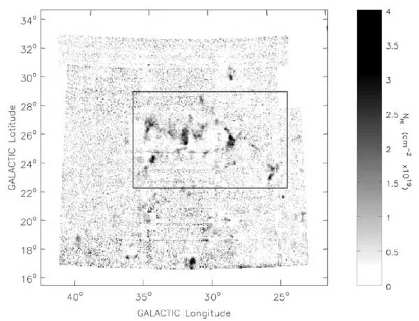
Figure 2: “The Plume” in H I  . An H I  column density map derived from GBT spectra integrated over $60\leq V_{\rm LSR}\leq 100$ km s${}^{-1}\>$. The figure shows an object which we call “the Plume.” It has peak H I  column densities of 2 – 4 $\times 10^{19}$ cm${}^{-2}\>$. The main part of it lies within the box, but there are a few separate clouds nearby with similar kinematics which are likely part of it. The cloud at $(\ell,b)\approx(29\arcdeg,31\arcdeg)$ is the highest-latitude member of this group discovered so far.

References

- Asgekar et al. (2005) Asgekar, A., English, J., Safi-Harb, S., & Kothes, R. 2005, AJ, 130, 674
- de Avillez & Berry (2001) de Avillez, M. A. & Berry, D. L. 2001 MNRAS, 328, 708
- de Avillez & Mac Low (2001) de Avillez, M. A. & Mac Low, M. M. 2001, ApJ, 551, L57
- Barnabè et al. (2006) Barnabè, M., Ciotti, L., Fraternali, F., & Sancisi, R. 2006, A&A, 446, 61
- Basu et al. (1999) Basu, S., Johnstone, D., & Martin, P. G. 1999, ApJ, 516, 843
- Bingham (1967) Bingham, R. G. 1967, MNRAS, 137, 157
- Bisnovatyj-Kogan & Silich (1995) Bisnovatyj-Kogan, G. S. & Silich, S. A. 1995, Rev. Mod. Phys., 67, 661
- Bissantz et al. (2003) Bissantz, N., Englmaier, P., & Gerhard, O. 2003, MNRAS, 340, 949
- Bland-Hawthorn & Maloney (2002) Bland-Hawthorn, J., & Maloney, P. R. 2002, in ASP Conf. Ser. 254, Extragalactic Gas at Low Redshift, ed. J. S. Mulchaey & J. Stocke (San Francisco: ASP), 267
- Breitschwerdt & de Avillez (2006) Breitschwerdt, D. & de Avillez, M. A. 2006 A&A, 452, L1
- Brinks & Bajaja (1986) Brinks, E. & Bajaja, E. 1986, A&A, 169, 14
- Burton & Gordon (1978) Burton, W. B. & Gordon, M. A. 1978, A&A, 63, 7
- Callaway et al. (2000) Callaway, M. B., Savage, B. D., Benjamin, R. A., Haffner, L. M., & Tufte, S. L. 2000, ApJ, 532, 943
- Castor et al. (1975) Castor, J., McCray, R., & Weaver, R. 1975, ApJ, 200, L107
- Clemens (1985) Clemens, D. P. 1985, ApJ, 295, 422
- Collins et al. (2002) Collins, J. A., Benjamin, R. A., & Rand, R. J. 2002, ApJ, 578, 98
- Cooper et al. (2004) Cooper, R. L., Guerrero, M. A., Chu, Y.-H., Chen, C.-H. R., & Dunne, B. C. 2004 ApJ, 605, 751
- Dehnen & Binney (1998) Dehnen, W. & Binney, J. 1998, MNRAS, 294, 429
- Dickey & Lockman (1990) Dickey, J. M. & Lockman, F. J. 1990, ARA&A, 28, 215
- Diplas & Savage (1994) Diplas, A., & Savage, B. D. 1994, ApJ, 427, 274
- Dove et al. (2000) Dove, J. B., Shull, J. M., & Ferrara, A. 2000, ApJ, 531, 846
- Ehlerová & Palouš (2005) Ehlerová, S. & Palouš, J. 2005, A&A, 437, 101
- Elmegreen & Lada (1977) Elmegreen, B. G. & Lada, C. J. 1977 ApJ, 214, 725
- English et al. (2000) English, J., Taylor, A. R., Mashchenko, S. Y., Irwin, J. A., Basu, S., & Johnstone, D. 2000, ApJ, 533, L25
- Fraternali & Binney (2006) Fraternali, F. & Binney, J. J. 2006, MNRAS, 366, 449
- Haffner et al. (1998) Haffner, L. M., Reynolds, R. J., & Tufte, S. L. 1998, ApJ, 501, L83
- Haffner et al. (2003) Haffner, L. M., Reynolds, R. J., Tufte, S. L., Madsen, G. J., Jaehnig, K. P., & Percival, J. W. 2003, ApJS, 149, 405
- Hartmann & Burton (1997) Hartmann, D. & Burton, W. B. 1997, Atlas of Galactic Neutral Hydrogen, (Cambridge, UK: Cambridge University Press)
- Haslam et al. (1982) Haslam, C. G. T., Salter, C. J., Stoffel, H., & Wilson, W. E. 1982, A&AS, 47, 1
- Heiles (1979) Heiles, C. 1979, ApJ, 229, 533
- Heiles (1984) Heiles, C. 1984, ApJS, 55, 585
- Howk & Savage (2000) Howk, J. C., & Savage, B. D. 2000, AJ, 119, 644
- Hu (1981) Hu, E. M. 1981, ApJ, 248, 119
- Igumenshchev et al. (1990) Igumenshchev, I. V., Shustov, B. M., & Tutukov, A. V. 1990 A&A, 234, 396
- Kim et al. (1999) Kim, S., Dopita, M. A., Staveley-Smith, L., & Bessell, M. S. 1999, AJ, 118, 2797
- Kompaneets (1960) Kompaneets, A. S. 1960, Soviet Phys. Dokl., 5, 46
- Koo et al. (1992) Koo, B.-C., Heiles, C., & Reach, W. T. 1992, ApJ. 390, 108
- Koo & McKee (1990) Koo, B.-C. & McKee, C. F. 1990, ApJ, 354, 513
- Koo & McKee (1992a) Koo, B.-C. & McKee, C. F. 1992, ApJ, 388, 93
- Koo & McKee (1992b) Koo, B.-C. & McKee, C. F. 1992, ApJ, 388, 103
- Korpi et al. (1999) Korpi, M. J., Brandenburg, A., Shukurov, A., & Tuominen, I. 1999, A&A, 350, 230
- Kudoh & Basu (2004) Kudoh, T. & Basu, S. 2004, A&A, 423, 183
- Lockman (1984) Lockman, F. J. 1984, ApJ, 283, 90
- Lockman et al. (1986) Lockman, F. J., Jahoda, K., & McCammon, D. 1986, ApJ, 302, 432
- Lockman (1989) Lockman, F. J. 1989, ApJS, 71, 469
- Lockman (2002a) Lockman, F. J. 2002, ApJ, 580, L47
- Lockman (2002b) Lockman, F. J. 2002, in ASP Conf. Ser. 278, Single-Dish Radio Astronomy: Techniques and Applications, ed. S. Stanimirovic et al. (San Francisco: ASP), 397
- Lockman & Pidopryhora (2005) Lockman, F. J. & Pidopryhora, Y. 2005, in ASP Conf. Ser. 331, Extra-planar Gas, ed. R. Braun (San Francisco: ASP), 59
- Lockman & Condon (2005) Lockman, F. J. & Condon, J. J. 2005, AJ, 129, 1968
- Maciejewski et al. (1996) Maciejewski, W., Murphy, E. M., Lockman, F. J., & Savage, B. D. 1996, ApJ, 469, 238
- Mac Low & McCray (1988) Mac Low, M. M. & McCray, R. 1988, ApJ, 324, 776
- Mac Low et al. (1989) Mac Low, M. M., McCray, R., & Norman, M. L. 1989, ApJ, 337, 141
- Madsen & Reynolds (2005) Madsen, G. J. & Reynolds, R. J. 2005, ApJ, 630, 925
- Martins et al. (2005) Martins, F., Schaerer, D., & Hillier, D. J. 2005, A&A, 436, 1049
- Matsushita et al. (2005) Matsushita, S., Kawabe, R., Kohno, K., Matsumoto, H., Tsuru, T. G., & Vila-Vilaró, B. 2005, ApJ, 618, 712
- McClure-Griffiths et al. (2000) McClure-Griffiths, N. M., Dickey, J. M., Gaensler, B. M., Green, A. J., Haynes, R. F., & Wieringa, M. H. 2000, AJ, 119, 2828
- McClure-Griffiths et al. (2002) McClure-Griffiths, N. M., Dickey, J. N., Gaensler, B. M., & Green, A. J. 2002, ApJ, 578, 176
- McCray & Kafatos (1987) McCray, R. & Kafatos, M. 1987, ApJ, 317, 190
- Motte et al. (2003) Motte, F., Schilke, P., & Lis, D. C. 2003, ApJ, 582, 277
- Oey & Clarke (1997) Oey, M. S. & Clarke, C. J. 1997, MNRAS, 289, 570
- Oey (2004) Oey, M. S. 2004, Ap&SS, 289, 269
- Oey & García-Segura (2004) Oey, M. S. & García-Segura, G. 2004, ApJ, 613, 302
- Pikel’ner & Shcheglov (1969) Pikel’ner, S. B. & Shcheglov, P. V. 1969, Soviet Astronomy, 12, 757
- Putman et al. (2003) Putman, M. E., Bland-Hawthorn, J., Veilleux, S., Gibson, B. K., Freeman, K. C., & Maloney, P. R. 2003, ApJ, 597, 948
- Reynolds (1985) Reynolds, R. J. 1985, ApJ, 294, 256
- Sancisi (1999) Sancisi, R. 1999, Ap&SS, 269, 59
- Savage et al. (1990) Savage, B. D., Massa, D., & Sembach, K. 1990, ApJ, 355, 114
- Savage et al. (1997) Savage, B. D., Sembach, K. R., & Lu, L. 1997, AJ, 113, 2158
- Savage et al. (2001) Savage, B. D., Sembach, K. R., & Howk, J. C. 2001, ApJ, 547, 907
- Smith et al. (1978) Smith, L. F., Biermann, P., & Mezger, P. G. 1978, A&A, 66, 65
- Smith (2006) Smith, N. 2006, MNRAS, 367, 763
- Snowden et al. (1997) Snowden, S. L., Egger, R., Freyberg, M. J., Plucinsky, P. P., Schmitt, J. H. M. M., Trümper, J., Voges, W., McCammon, D., & Sanders, W. T. 1997, ApJ, 485, 125
- Stanimirovic et al. (1999) Stanimirovic, S., Staveley-Smith, L., Dickey, J. M., Sault, R. J., & Snowden, S. L. 1999, MNRAS, 302, 417
- Staveley-Smith et al. (1997) Staveley-Smith, L., Sault, R. J., Hatzidimitriou, D., Kesteven, M. J., & McConnell, D. 1997, MNRAS, 289, 225
- Tenorio-Tagle et al. (1987) Tenorio-Tagle, G., Bodenheimer, P., & Rozyczka, M. 1987 A&A, 182, 120
- Tenorio-Tagle & Bodenheimer (1988) Tenorio-Tagle, G. & Bodenheimer, P. 1988 ARA&A, 26, 145
- Tenorio-Tagle et al. (1990) Tenorio-Tagle, G., Rozyczka, M., & Bodenheimer, P. 1990 A&A, 237, 207
- Tomisaka & Ikeuchi (1986) Tomisaka, K. & Ikeuchi, S. 1986, PASJ, 38, 697
- Tomisaka (1998) Tomisaka, K. 1998 MNRAS, 298, 797
- Tripp et al. (2003) Tripp, T. M., Wakker, B. P., Jenkins, E. B., Bower, C. W., Danks, A. C., Green, R. F., Heap, S. R., Joseph, C. L., Kaiser, M. E., Linsky, J. L., & Woodgate, B. E. 2003, AJ, 125, 3122
- Tufte et al. (1998) Tufte, S. L., Reynolds, R. J., & Haffner, L. M. 1998, ApJ, 504, 773
- Tufte et al. (2002) Tufte, S. L., Wilson, J. D., Madsen, G. J., Haffner, L. M., & Reynolds, R. J. 2002, ApJ, 572, L153
- Veilleux et al. (2005) Veilleux, S., Cecil, G., & Bland-Hawthorn, J. 2005, ARA&A, 43, 769
- Voit (1988) Voit, G. M. 1988, ApJ, 331, 343
- Walter & Brinks (1999) Walter, F. & Brinks, E. 1999, AJ118, 273
- Weaver et al. (1977) Weaver, R., McCray, R., Castor, J., Shapiro, P., & Moore, R. 1977, ApJ, 218, 377
- Weiß et al. (1999) Weiß, A., Walter, F., Neininger, N, & Klein, U. 1999, A&A, 345, L23
- Williams (1973) Williams, D. R. W. 1973, A&AS, 8, 505
- Willingale et al. (2003) Willingale, R., Hands, A. D. P., Warwick, R. S., Snowden, S. L., & Burrows, D. N. 2003, MNRAS, 343, 995
- Wolfire et al. (1995) Wolfire, M. G., McKee, C. F., Hollenbach, D., & Tielens, A. G. G. M. 1995, ApJ, 453, 673