The fraction of DA white dwarfs with kilo-Gauss magnetic fields

Abstract

Context. Weak magnetic fields have been searched for on only a small number of white dwarfs. Current estimates find that about 10% of all white dwarfs have fields in excess of 1 MG; according to previous studies this number increases up to about 25% in the kG regime.

Aims. Our aim is to improve on these statistics by a new sample of ten white dwarfs in order to determine the ratio of magnetic to field-free white dwarfs.

Methods. Mean longitudinal magnetic fields strengths were determined by means of high-precision circular polarimetry of H$\beta$ and H$\gamma$ with the FORS1 spectrograph of the VLT “Kueyen” 8 m telescope.

Results. In one of our objects (LTT 7987), we detected a statistically significant (97% confidence level) longitudinal magnetic field varying between ($-1\pm 0.5$) kG and ($+1\pm 0.5$) kG. This would be the weakest magnetic field ever found in a white dwarf, but systematic errors cannot completely be ruled out at this level of accuracy. We also observed the sdO star EC 11481-2303 but could not detect a magnetic field.

Conclusions. VLT observations with uncertainties typically of 1000 G or less suggest that 15$-$20% of WDs have kG fields. Together with previous investigations, the fraction of kG magnetic fields in white dwarfs amounts to about 11$-$15%, which is close to the current estimations for highly magnetic white dwarfs ($>$1 MG).

1 Introduction

The question how many white dwarfs are magnetic has been actively debated in the recent years. In about 170 of the 5500 white dwarfs listed in the online version of the Villanova White Dwarf Catalog (http://www.astronomy.villanova.edu/WDCatalog/index.html) magnetic fields between 2 kG and 1 GG have been measured, corresponding to a fraction of about 3% (McCook & Sion 1999; Wickramasinghe & Ferrario 2000; Vanlandingham et al. 2005). However, the spectra of only a few of the known white dwarfs have been examined for the presence of a magnetic field in enough detail. Liebert et al. (2003) and Schmidt et al. (2003) estimate that the true fraction of white dwarfs with magnetic fields in excess of 2 MG is expected to be at least $\approx 10\%$ and may be as high as 20%.

Until recently, magnetic fields below 30 kG could not be detected, with the exception of the very bright white dwarf 40 Eri B ($V=8.5$), in which Fabrika et al. (2003) found a magnetic field of 4 kG. However, by using the ESO VLT, we could push the detection limit down to about 1 kG in our first investigation of 12 DA white dwarfs with $11<V<14$ (Aznar Cuadrado et al. 2004). In 3 objects of this sample, we detected magnetic fields between 2 kG and 7 kG on a $5\sigma$ confidence level. Therefore, we concluded that the fraction of white dwarfts with kG magnetic fields is about 25%.

For one of our cases, LP 672$-$001 (WD 1105$-$048), Valyavin et al. (2006) confirm the presence of a kG magnetic field by measuring circular polarisation at H$\alpha$ using the 6m of the Special Astrophysical Observatory. On the other hand, none of the other 5 bright white dwarfs of their sample showed any significant signature of a magnetic field. They detected a magnetic field of up to 10 kG in the hot subdwarf (spectral type sdO) Feige 34, confirming the detection of magnetic fields in both types of white dwarf progenitors, hot subdwarfs (O’Toole et al. 2005) and central stars of planetary nebulae (Jordan et al. 2005).

With this new investigation, we increase the sample of white dwarfs that is checked for kG magnetic fields by means of circular polarisation by eleven objects (one turned out to be a high-metallicity sdO, Stys et al. (2000)). This should allow us to provide a much better estimate of the incidence of low magnetic fields in white dwarfs.

All tables have been organised in exactly the same way as in Aznar Cuadrado et al. (2004, Paper I); the figures show the same spectral regions as in Paper I but have been plotted in a more compact way.

2 Observations and data reduction

The spectropolarimetric data of our new sample of ten bright normal DA white dwarfs plus one high-metallicity sdO star were obtained in service mode between May 5 and August 4, 2004, with the FORS1 spectrograph at the 8 m UT2 (“Kueyen”) of the VLT. The setup was exactly the same as described in Paper I. The spectra and circular polarimetric data covered the wavelength region between 3600 Å and 6000 Å with a spectral resolution of 4.5 Å. A higher spectral resolution would not provide a higher sensitivity since the accuracy is basically limited by the signal-to-noise ratio allone. The exposures were split into a sequence of exposures to avoid saturation; after every second observation the retarder plate was rotated from $\alpha=-45^{\circ}$ to $\alpha=+45^{\circ}$ and back in order to suppress spurious signals in the degree of circular polarisation (calculated from the ratio of the Stokes parameters $V$ and $I$). All stars were observed in two or three different nights in order to detect the presence of possible variations in $V/I$ due to the rotation of the stars.

As in the case of the sample of Paper I, all objects in our new sample of DA white dwarfs have been previously observed in the course of the SPY survey (Napiwotzki et al. 2003), a radial velocity search for close binary systems composed of two white dwarfs. We checked all candidates for spectral peculiarities and magnetic fields strong enough to be detected in intensity spectra taken with the high-resolution Echelle spectrograph UVES at the Kueyen (UT2) of the VLT. None of our programme stars showed any sign of Zeeman splitting in the SPY SURVEY, i.e., indicating that any possible magnetic field must be below a level of about 20 kG.

The data reduction and calculation of the observed circular polarisation is described in detail in Paper I. Special care was taken to avoid errors from changes in the sky transparency, atmospheric scintillation, and various instrumental effects. The wavelength calibration was made for each observing date separately, and no spurious signals were detected during the calibration process.

Details of our eleven sample stars and of our observations are listed in Table 1. The provided $\alpha$ and $\delta$ coordinates refer to epoch 2000 as measured in the course of the SPY project (see Koester et al. 2001). Spectral types, $T_{\rm sp}$, and measured V magnitudes were taken from the catalogue of McCook & Sion (1999). EC 11481-2303 was classified as an DAO white dwarf by Kilkenny et al. (1997).

3 Determination of magnetic fields

As discussed in Paper I, the theoretical $V/I$ profile for a given mean longitudinal magnetic field $\langle B_{z}\rangle$ (expressed in Gauss) below about 10 kG is given by the weak-field approximation (e.g.  Angel & Landstreet 1970; Landi degl’Innocenti & Landi degl’Innocenti 1973) without any loss in accuracy:

$$\frac{V}{I}=-g_{\rm eff}C_{z}\lambda^{2}\frac{1}{I}\frac{\partial I}{\partial\lambda}\langle\large B_{z}\large\rangle\;,$$ (1)

where $g_{\rm eff}$ is the effective Landé factor (= 1 for all hydrogen lines of any series, Casini & Landi degl’Innocenti 1994), $\lambda$ is the wavelength expressed in Å, and the constant $C_{z}=e/(4\pi m_{e}c^{2})$ $(\simeq 4.67\times 10^{-13}\,{\rm G}^{-1}\mbox{\AA}^{-1})$.

We again performed a $\chi^{2}$-minimisation procedure to find out which mean longitudinal magnetic field strength fits the observed data best in wavelength intervals of $\pm$20 Å around H$\beta$ and H$\gamma$. Since the error of the magnetic field determination increases for the higher series number, we based our investigation only on these two Balmer lines.

The resulting best-fit values for the magnetic field strengths from the individual lines and their statistical $1\sigma$ errors are listed in Table 2 for each observation. $B({\sigma})$ provides the magnetic field in units of the $\sigma$ level. Detections exceeding the $2\sigma$ levels are given in bold. $\sigma(V)$ is the standard deviation of the observed ($V/I$)-spectrum obtained in the region 4500–4700 Å. Lower limits on the detectability of the magnetic field from the line polarisation peaks, calculated at the $1\sigma$ level of the noise, are given in the last two columns. Multiple observations that were averaged prior to analysis are labeled average. We also provid the weighted means $B_{z}=(B_{z,\gamma}w_{\gamma}+B_{z,\beta}w_{\beta})/(w_{\gamma}+w_{\beta})$ where $w_{i}=1/\sigma_{i}^{2}$ ($i=\gamma,\beta$). The probable error is given by $\sigma=(\sum w_{i})^{-1/2}$.

Moreover, we expressed the resulting mean magnetic field in multiples of the $1\sigma$ error in order to judge the significance of the magnetic field determination. For a comparison we note that for each of the three stars with significant magnetic fields from the Aznar Cuadrado et al. (2004) sample, at least one observation exceeded the $5\sigma$ level.

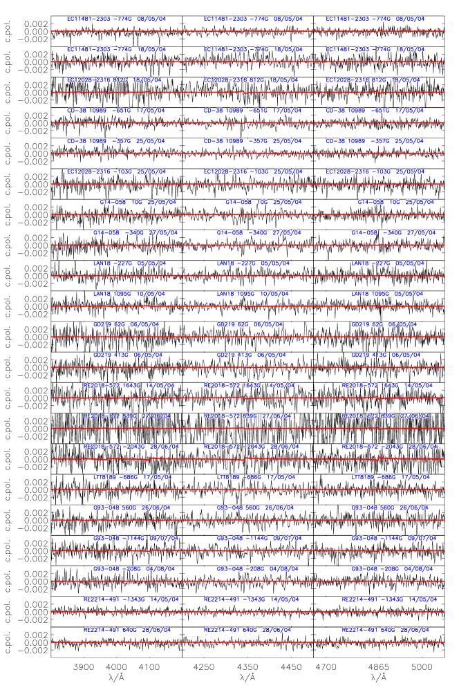
Figure 3: Circular polarisation spectra $V/I$ (thin black lines) for different observing dates in the regions around H$\beta$ (4861Å, right), H$\gamma$ (4340 Å, middle), and close to the Balmer threshold (left) for those measurements, where no significant magnetic field could be detected. The red thick lines represent the circular polarisation predicted by the low-field approximation (Eq. 1) using the values for the longitudinal magnetic field from the best fit to the H$\beta$ and H$\gamma$ regions.

In Table 2 we also calculated lower limits on the detectability of the magnetic fields from the line polarisation peaks, which guide the eye when judging the confidence of the fits from plots of the circular polarisation (Fig.1 and online Fig.3). Note, however, that a significant contribution to the fit originates not only from the narrow peaks but also from the full 40 Å interval around the Balmer lines. Note, however, that in the three magnetic cases of our first study, the S-wave circular polarisation signature reaches the $2\sigma$ level of the noise. For each object we also added up all measurements according to formula 3 in Paper I. The results for these added observations were labeled as average.

Our fitting procedure was validated with extensive numerical simulations using a large sample of 1000 artificial noisy polarisation spectra (Aznar Cuadrado et al. 2004). It was found that at our noise level $\sigma(V)$ (also listed in Table 2) of some $10^{-3}I_{\rm c}$ ($I_{\rm c}$ being the continuum intensity), kG fields can reliably be detected.

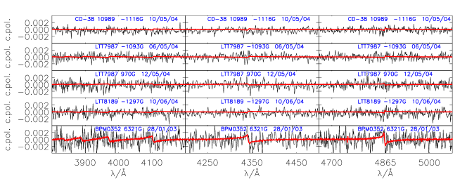
Figure 1: Circular polarisation spectra $V/I$ (thin black lines) around H$\beta$ (4861Å, right), H$\gamma$ (4340 Å, middle), and close to the Balmer threshold (left) for those observations, where the $2\sigma$ level is exceeded. The thick lines (red in the online version) represent the circular polarisation predicted by the low-field approximation (Eq. 1), using the values for the longitudinal magnetic field from the best fit to the H$\beta$ and H$\gamma$ regions. For comparison we also plotted the result for BPM 0352 with $B=6321$ G (lowest panel), which was analysed by Aznar Cuadrado et al. (2004). The plots of all other observations are shown in Fig. 3 of the online version.

Figure 2: Temperature-gravity diagram with the positions of white dwarfs analysed in Paper I and in the current paper. Theoretical cooling sequences from Benvenuto & Althaus (1999) are plotted for various white dwarf masses. White dwarfs with and without detected magnetic fields are indicated by different symbols. The double-lined binary WD 0135$-$052 from Paper I is not shown in this plot.

Table 1: Details of the VLT observations.

Target	Alias	$\alpha$	$\delta$	V	HJD	$t_{\rm exp}$	$n$	$T_{sp}$
				(mag)	(+2453000)	(s)
WD 1148$-$230	EC 11481$-$2303	11 50 38.85	$-$23 20 34.8	11.76	134.096	150	10	sdO
					144.097	150	8
WD 1202$-$232	EC 12028$-$2316	12 05 26.80	$-$23 33 14.0	12.79	144.132	500	4	DA
					151.983	500	4
WD 1327$-$083	G 14$-$058	13 30 13.58	$-$08 34 30.2	12.31	151.519	290	6	DA3.5
					153.554	285	6
WD 1620$-$391	CD$-$38 10980	16 23 33.84	$-$39 13 46.2	11.00	136.285	73	14	DA
					143.323	73	14
					151.054	73	14
WD 1845$+$019	Lan 18	18 47 39.09	$+$01 57 33.8	12.95	131.878	350	6	DA1.5
					136.873	285	6
WD 1919$+$145	GD 219	19 21 40.51	$+$14 40 40.5	12.94	132.808	350	6	DA5
					136.834	350	6
WD 2007$-$303	LTT 7987	20 10 56.82	$-$30 13 06.7	12.18	132.848	300	12	DA4
					138.858	300	6
WD 2014$-$575	RE 2018$-$572	20 18 54.88	$-$57 21 33.8	13.00	140.842	350	6	DA2
					184.757	350	2
					185.591	350	6
WD 2039$-$202	LTT 8189	20 42 34.64	$-$20 04 35.6	12.33	143.847	300	6	DA2.5
					167.879	300	6
WD 2149$+$021	G 93$-$048	21 52 25.43	$+$02 23 17.8	12.72	183.762	348	6	DA3
					196.829	348	6
					222.684	348	6
WD 2211$-$495	RE 2214$-$491	22 14 11.93	$-$49 19 27.1	11.70	140.885	161	10	DA1
					185.730	161	10

Table 2: Magnetic fields derived from the H$\gamma$ and H$\beta$ lines for our sample of white dwarfs.

Target	Date	$\sigma(V)$	$B$(G)		$B({\rm G})$	$B({\sigma})$	B(G) at $1\sigma$
		(10${}^{-3}I_{\rm c}$)	H$\gamma$	H$\beta$	H$\gamma,\beta$	H$\gamma,\beta$	H$\gamma$	H$\beta$
WD 11481$-$2303	08/05/04	0.7	$-520\pm 655$	$-980\pm 590$	$-774\pm 438$	1.76	$-$1970	$-$1480
	18/05/04	1.0	$-30\pm 1325$	$20\pm 1095$	$0\pm 844$	0.00	3060	2310
	average	0.6	$-490\pm 625$	$-860\pm 500$	$-716\pm 390$	1.83	$-$1650	$-$1260
WD 1202-232	18/05/04	1.3	$1280\pm 865$	$260\pm 940$	$812\pm 636$	1.28	1560	1160
	25/05/04	1.2	$660\pm 550$	$-370\pm 325$	$-103\pm 280$	0.37	1260	960
	average	0.9	$-200\pm 260$	$850\pm 425$	$85\pm 221$	0.39	1040	770
WD 1327-083	25/05/04	0.8	$300\pm 1010$	$-320\pm 1080$	$10\pm 737$	0.01	2110	$-$1690
	27/05/04	1.1	$-2800\pm 740$	$2790\pm 835$	$-340\pm 553$	0.61	$-$2700	2220
	average	0.7	$-1230\pm 555$	$1410\pm 520$	$175\pm 379$	0.46	$-$1630	1330
WD 1620-391	10/05/04	0.6	$150\pm 785$	$-1580\pm 475$	$-$1116$\pm$ 406	2.75	-1900	$-$1330
17/05/04	0.7	$-2390\pm 1220$	$-20\pm 735$	$-651\pm 629$	1.03	-2150	$-$1490
	25/05/04	0.6	$120\pm 640$	$-770\pm 595$	$-357\pm 435$	0.82	$-$1990	$-$1440
	average	0.4	$-500\pm 480$	$-920\pm 365$	$-$766$\pm$290	2.63	1310	910
WD 1845+019	05/05/04	1.1	$-340\pm 1410$	$-150\pm 1175$	$-227\pm 902$	0.25	$-$4660	$-$3710
	10/05/04	0.9	$-30\pm 1145$	$6000\pm 2390$	$1095\pm 1032$	1.06	$-$3930	2930
	average	0.8	$-130\pm 815$	$500\pm 670$	$245\pm 517$	0.47	$-$3310	2510
WD 1919+145	06/05/04	1.6	$1240\pm 1080$	$-1440\pm 1220$	$62\pm 808$	0.08	4590	$-$3610
	10/05/04	1.2	$930\pm 1290$	$110\pm 990$	$413\pm 785$	0.53	3340	2650
	average	1.0	$1180\pm 870$	$-500\pm 815$	$285\pm 594$	0.48	2760	$-$2150
WD 2007$-$303	06/05/04	0.7	$-1460\pm 1270$	$-1040\pm 485$	$-$1093$\pm$ 453	2.41	$-$1780	$-$1280
	12/05/04	0.8	$1540\pm 780$	$610\pm 620$	970$\pm$485	2.00	2270	1640
	average	0.5	$120\pm 495$	$-390\pm 375$	$-204\pm 298$	0.67	1460	$-$1090
WD 2014-575	14/05/04	1.6	$2410\pm 1735$	$1240\pm 1260$	$1643\pm 1019$	1.61	5340	3950
	27/06/04	3.4	$310\pm 4295$	$1160\pm 3340$	$839\pm 2636$	0.32	11680	7720
	28/06/04	1.8	$2820\pm 2060$	$-4470\pm 1455$	$-2043\pm 1188$	1.71	6330	$-$4130
	average	1.3	$2380\pm 1205$	$-1120\pm 895$	$124\pm 718$	0.17	3740	$-$2680
WD 2039-202	17/05/04	1.4	$-2670\pm 1595$	$40\pm 965$	$-686\pm 825$	0.83	$-$3650	2780
	10/06/04	0.8	$-780\pm 730$	$-1800\pm 720$	$-$1297$\pm$512	2.53	$-$2370	$-$1670
	average	0.6	$-1240\pm 655$	$-1290\pm 535$	$-$1269$\pm$414	3.06	$-$1810	$-$1300
WD 2149+021	26/06/04	2.1	$340\pm 1060$	$730\pm 930$	$560\pm 699$	0.80	6570	4450
	09/07/04	1.1	$-530\pm 945$	$-1690\pm 890$	$-1144\pm 647$	1.78	$-$3620	$-$2420
	04/08/04	0.8	$-1300\pm 985$	$350\pm 705$	$-208\pm 573$	0.36	$-$2330	1520
	average	0.9	$-600\pm 555$	$-130\pm 490$	$-335\pm 367$	0.91	$-$1730	$-$1150
WD 2211-495	14/05/04	0.7	$110\pm 1655$	$-1940\pm 1060$	$-1343\pm 892$	1.51	7570	$-$4150
	28/06/04	0.7	$-190\pm 1795$	$640\pm 1190$	$386\pm 991$	0.39	8570	4470
	average	0.5	$-390\pm 1155$	$-900\pm 795$	$-736\pm 654$	1.12	$-$5830	$-$3050

Table 3: Fitted parameters of the white dwarfs and supplementary data from literature.

						literature
WD	Teff	$\log g$	$M$	$d$(spec)	$t_{\mathrm{cool}}$	$T_{\rm eff}$	$\log g$	$v\sin i$	$d$(trig)
	(kK)		(${\rm M}_{\odot}$)	(pc)	(Myr)	(kK)		(km s-1)	(pc)
WD 1202$-$232	8.75	8.11	0.663	9.9	1052	8.62	8.007	$<6$7
WD 1327$-$083	14.83	7.83	0.518	18.1	157	14.41	7.851		$18.0\pm 1$2
WD1620$-$391	25.29	7.89	0.576	14.9	18	24.25	8.054	$<8$4	$12.8\pm 0.4$2
WD 1845$+$019	30.33	7.78	0.536	47.4	8	30.35	7.831
WD 1919$+$145	14.88	8.07	0.652	21.0	236	14.60	8.093	$<6$4	$20\pm 3$5
WD 2007$-$303	15.36	7.97	0.595	16.0	178	15.15	7.861	$<7$4	$15\pm 1$2
WD 2014$-$575	27.99	7.82	0.548	57.8	11	28.37	7.871	$<14$4
WD 2039$-$202	19.79	7.77	0.502	24.2	46	20.41	7.841	$<15$4	$21\pm 2$2
WD 2149$+$021	17.53	7.89	0.557	24.2	96	17.65	7.991		$25\pm 3$2
WD 2211$-$495	68.11	7.43	0.518	67.3	0.1	66.50	7.526

References: ¹Bragaglia et al. (1995); ²Perryman et al. (1997); ³Koester et al. (1998); ⁴Karl et al. (2005); ⁵van Altena et al. (1995); ⁶Finley et al. (1997); ⁷Berger et al. (2005).

4 Results

EC 11481$-$2303 (WD1148$-$230) is a high-gravity pre-white dwarf of spectral type sdO, which we disregard n our statistics on white dwarfs, but whose measurement is intersting on its own. The nature of this star with $T_{\rm eff}=42\,000$ K and $\log g=5.8$ has been revealed by Stys et al. (2000).

As can be seen from Table 2, Fig. 1, and Fig. 3 (online only), none of the measurements of the circular polarisations reached the same level of confidence as the three magnetic objects found in the first sample (Paper I). The highest level of confidence was achieved by LTT 7987 (WD 2007$-$303) where a $2.4$ and $2.0\sigma$ level was reached for the two respective observations. The corresponding mean longitudinal field strengths were $-1093\pm 453$ G and $970\pm 485$ G. Single observations of CD$-$38 10980 (WD162$-$391) resulted in $-1116\pm 406$ G and LTT 8189 (WD 2039$-$202) in $-1297\pm 512$ G, which corresponds to $2.8\sigma$ and $2.5\sigma$, respectively.

In Paper I we disregarded the case of LHS 1270, for which a magnetic field of $654\pm 320$ G was found. Since their sample consisted of 22 single observations, statistically one would expect this $2\sigma$ observation even if all the stars have no magnetic field.

Our new sample consists of 23 single observations of white dwarfs and two observations of a metal-rich sdO. With the same argument we would statistically expect only one observation to exceed the $2\sigma$ level. Therefore, one can assume that between none and three of the observations may actually be a real observation.

With two observations exceeding $2\sigma$, LTT 7987 (WD 2007$-$303) would be the most convincing for a positive detection. The probability that two independent and uncorrelated observations of a single star have that level of confidence can be estimated in the following way: The likelihood that an observation exceeds 2$\sigma$ is 4.6%; therefore, the chance that at least one observation of the white dwarfs exceeds 2$\sigma$ is $(1-0.954^{23})=66.1$%. Then the probability that the same star has a second observation exceeding 2$\sigma$ is $0.661\cdot 0.046=3.0$%. Therefore, from a purely statistical point of view, we must regard this detection as significant (with 97% confidence).

However, we have to take into account that the measured magnetic field strengths would be only about 1 kG, which is 2 to 6 times smaller than the positive detections from the sample of Paper I. At this level we cannot fully exclude systematic errors from the limitation of our low-field approximation (assuming a single magnetic strength rather than a distribution) or from instrumental polarisation. However, Bagnulo et al. (2006) have shown that none of their observed non-magnetic A stars – observed with the same instrument – showed circular polarization hinting at magnetic fields larger than 400 G. This would mean that the systematic errors are well below 1 kG.

On the other hand, none of the polarisation peaks of LTT 7987 in Fig. 1 exceeds the noise level, differently from the three detections BPM 03523, LP 672$-$001, and L 362$-$434 in Aznar Cuadrado et al. (2004). Therefore, a $\chi$-by-eye analysis would not confirm our detection but, as we pointed out in Paper I, this would be very misleading.

Both measurements of the sdO star EC 11481-2303 are below the $2\sigma$ level. This is interesting in itself and confirms the finding by O’Toole et al. (2005) that there is no correlation between the metallicity and the presence of a magnetic field with kG strength. Therefore, we conclude that although the measured magnetic field in LTT 7987 is statistically significant, further observations are needed to establish their reality.

In order to find out whether white dwarfs with and without kG magnetic fields differ in mass or age, we computed masses and cooling ages from the fundamental atmospheric parameters temperature and gravity. The values of $T_{\rm eff}$ and $\log g$ were derived from a model atmosphere analysis of the high signal-to-noise spectra (see Fig. 4 in the online material). The observed line profiles are fitted with theoretical spectra from a large grid of NLTE spectra calculated with the NLTE code developed by Werner (1986). The four coolest white dwarfs of our sample (WD 1327$-$083, WD 1919$+$145, and WD 2007$-$303) were analysed with a grid of LTE model spectra computed by D. Koester for the analysis of DA white dwarfs (see e.g.  Finley et al. 1997), which is more reliable below 17000 K, where convection and collision-induced absorption by hydrogen quasi-molecules play a role.

Table 3 lists the results of the model atmosphere analyses. From these we determined spectroscopic distances, as well as masses and cooling ages computed from a comparison of parameters derived from the fit with the grid of white dwarf cooling sequences by Benvenuto & Althaus (1999), for an envelope hydrogen mass of $10^{-4}M_{\mathrm{WD}}$. A temperature-gravity diagram with the positions of white dwarfs analysed in Paper I and in the current paper is shown in Fig. 2. In Table 3 we also provid data collected from the literature (atmospheric parameters, rotational velocities, and trigonometic parallaxes) when available.

5 Conclusion

While we detected magnetic fields in 3 out of the 12 programme stars in our first investigation, we found at most (if at all) one object in our new sample of 10 DA white dwarfs. Putting both samples together, we arrive at a fraction of 14$-$18%  of kG magnetism in white dwarfs; the lower value is obtained assuming that LTT 7987 is not magnetic. However, if confirmed, LTT 7987 would have the lowest magnetic field (1 kG) ever detected in a white dwarf.

Recently, Valyavin et al. (2006) also performed a search for circular polarisation in white dwarfs. They confirmed our detection (Aznar Cuadrado et al. 2004) of a varying longitudinal magnetic field in LP 672$-$001 (WD 1105$-$048): they measured field strengths between $-7.9\pm 2.6$ kG to $0.1\pm 2.7$ kG, compared to our values of $-4.0\pm 0.7$ kG to $-2.1\pm 0.4$ kG. However, they did not discover any significant magnetic field in their five other programme stars. If we combine their results with our’s, the fraction of kG magnetic fields in DA white dwarfs amounts to 15% (4/(12+10+5)) or 11% (3/(12+10+5)), if we disregard the detection in LTT 7987. However, it is problematic to merge both samples, because the signal-to-noise ratio of our VLT measurements is much higher than the observations with the 6 m telescope of the Special Astrophysical Observatory. Since our uncertainties are on the average 2$-$3 times smaller (partly also due to the fact that Valyavin et al. (2006) only used H$\alpha$), we must put a higher statistical weight on our sample with a fraction of 11% to 15% of magnetic to field-free (i.e. below detection limit) white dwarfs.

While one of the white dwarfs with a magnetic field (L 362$-$81) had an exceptionally high mass (0.95 $M_{\odot}$), all objects with kG magnetic fields have usual white dwarf masses in the range 0.5 to 0.6 $M_{\odot}$. Therefore, a trend towards higher masses in magnetic white dwarfs compared to non-magnetic ones (Liebert 1988) does not seem to exist for magnetic white dwarfs with kG fields. This would be consistent with the idea that the high-magnetic-field white dwarfs have a higher-than-average mass because they have more massive progenitors. Therefore, it is probable that the white dwarfs with kG magnetic fields stem from a low-mass progeny on the main sequence (e.g.  F stars) as speculated by Wickramasinghe & Ferrario (2005).

Appendix A Figures in the electronic version

Two figures are only available in the electronic online version of the paper.

Figure 4: Model atmosphere fits (solid line) for the mean of all measured spectra (dashed line) of the white dwarfs. The results for $T_{\rm eff}$ and $\log g$ are given in Table 3.