Power Laws and the Cosmic Ray Energy Spectrum

Abstract

Two separate statistical tests are applied to the AGASA and preliminary Auger Cosmic Ray Energy spectra in an attempt to find deviation from a pure power-law. The first test is constructed from the probability distribution for the maximum event of a sample drawn from a power-law. The second employs the TP-statistic, a function defined to deviate from zero when the sample deviates from the power-law form, regardless of the value of the power index. The AGASA data show no significant deviation from a power-law when subjected to both tests. Applying these tests to the Auger spectrum suggests deviation from a power-law. However, potentially large systematics on the relative energy scale prevent us from drawing definite conclusions at this time.

1 Introduction

Nature offers a wide range of phenomena characterized by power-law distributions: diameter of moon craters, intensity of solar flares, the wealth of the richest people[1] and intensity of terrorist attacks[2], to name a few. These distributions are so-called heavy-tailed, where the fractional area under the tail of the distribution is larger than that of a gaussian and there is thus more chance for samples drawn from these distributions to contain large fluctuations from the mean. Anatomical defects aside, the cosmic ray (CR) energy spectrum follows a power-law for over ten orders of magnitude. The predicted abrupt deviation at the very highest energies (the GZK-cutoff[3, 4]) has generated a fury of theoretical and experimental work in the past half century. Recently, Bahcall[5] and Waxman (2003) have asserted that the observed spectra (except AGASA) are consistent with the expected flux suppression above $5\times 10^{19}$eV. However, the incredibly low fluxes combined with as much as $\sim$50% uncertainty in the absolute energy determination means that there has yet to be a complete consensus on the existence of the GZK-cutoff energy.

With this in mind, we consider statistics which suggest an answer to a different question: Do the observed CR spectra follow a power-law? Specifically, these studies are designed to inquire whether or not there is a flux deviation relative to the power-law form by seeking to minimize the influence of the underlying parameters.

The two experimental data sets considered in this study are the AGASA[8] experiment and the preliminary flux result of the Pierre Auger Observatory[6, 7]. The discussion in $\S$2 uses these spectra to introduce and comment on the power-law form. The first distinct statistical test is applied to this data in $\S$3 where we explore the distribution of the largest value of a sample drawn from a power-law. In $\S$4 we apply the TP-statistic to the CR flux data. This statistic is asymptotically zero for pure power-law samples regardless of the value power index and therefore offers a (nearly) parameter free method of determining deviation from the power-law form. The final section summarizes our results.

2 The Data

A random variable $X$ is said to follow a power-law distribution if the probability of observing a value between $x$ and $x+dx$ is $f(x)dx$ where $f(x)=Cx^{-{\gamma}}$. Normalizing this function such that $\int_{x_{min}}^{\infty}f(x)dx=1$ gives,

$$f_{X}(x)=\frac{{\gamma}-1}{x_{min}}\left(\frac{x}{x_{min}}\right)^{-{\gamma}}.$$ (1)

It is convenient to choose $z=x/x_{min}\Rightarrow dz=dx/x_{min}$, $1\leq z<\infty$ and doing so yields

$$f_{Z}(z)=({\gamma}-1)z^{-{\gamma}}.$$ (2)

For reference, one minus the cumulative distribution function $F_{Z}(z)$ is given by,

$$1-F_{Z}(z)=\int_{z}^{\infty}f_{Z}(y)dy=z^{1-{\gamma}}.$$ (3)

Taking the log of both sides of equation (1) yields

$$\log f(x)=\log A-{\gamma}\log x,$$ (4)

where $A$ is an overall normalization parameter, and suggests a method of estimating ${\gamma}$; the power index is the slope of the best fit line to the logarithmically binned data (i.e. bin-centers with equally spaced logarithms). In what follows, we refer to the logarithmically binned estimate[9] of the power index as ${\hat{\gamma}}$ and assume that the typical $\chi^{2}$/NDF is indicative of the goodness of fit. The fitting is done with two free parameters, namely $A$ and ${\gamma}$.

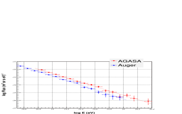
Figure 1: This figure displays published AGASA[8] and Auger[6] CR energy spectra. Both axis have logarithmic scales to illustrate the power-law behavior. The vertical axis is the flux $J$ in (m² sr sec eV)^-1 and the horizontal axis is the energy in eV. The best fit lines (see 4) have slope $\hat{{\gamma}}_{AGASA}=2.80\pm 0.23$ and $\hat{{\gamma}}_{Auger}=2.97\pm 0.12$ (statistical error only).

The energy flux of two publicly available data sets are shown in Fig. 1. The the red point-down triangles represent the log₁₀ of the binned AGASA flux values in units of (m² sr sec eV)^-1 and the blue point-up triangles correspond to the Auger flux. The vertical error bars on each bin reflect the Poisson error based on the number of events in that bin. The log-binned estimates for each complete CR data set are the slopes of the dashed lines plotted in Fig. 1.

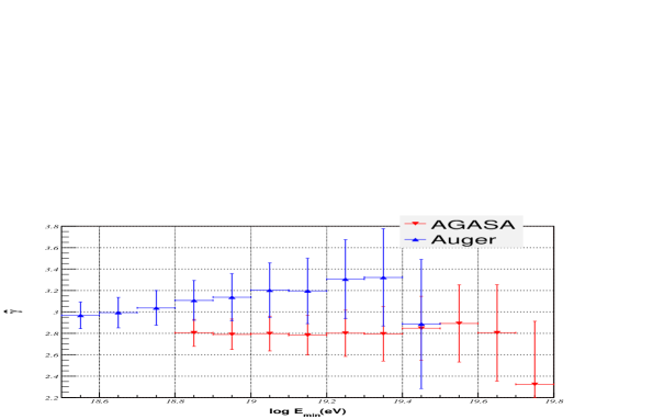
Figure 2: To check the stability of ${\hat{\gamma}}$ we estimate the power index as a function of the minimum energy $E_{min}$ considered for the AGASA and Auger CR data sets; see Fig.1. The left most point is the slope of the best fit lines plotted in Fig.1. The vertical error bars represent $1\sigma_{{\hat{\gamma}}}$ deviation.

In order to check the stability of to bound on our estimate, we compute the estimated power index ${\hat{\gamma}}$ as a function of the minimum energy $E_{min}$ considered for each of the two CR data sets. The left-most blue (red) point in Fig. 2 shows ${\hat{\gamma}}$ for the Auger (AGASA) data taking into account all of the bin values above $\log E_{min}=18.5$ ($\log E_{min}=18.8$), the next point to the right represents that for all bins above $\log E_{min}=18.6$ ($\log E_{min}=18.9$), and so on. The vertical error bars on these points represent the $1\sigma_{{\hat{\gamma}}}$ error of the estimate. To ensure an acceptable chi-squared statistic, we demand that at least five bins be considered, thereby truncating $E_{min}$ at $\log E_{min}=19.4$ for the Auger and $\log E_{min}=19.7$ for the AGASA data set. The $\chi^{2}$/NDF for the left-most points is $\sim 0.3$ and it increases to $\sim 2.5$ for the right-most for both experiments. We note that these estimates do not vary widely for the lowest $E_{min}$’s and that the values of ${\hat{\gamma}}$ from these experiments are consistent.

The analyses discussed in $\S$3 and $\S$4 will depend on the total number of events in the data set. Since these numbers are not published we use a simple method for estimating them from the CR flux data. If the exposure is a constant function of the energy, then we may take the flux $J$ to be proportional to the number of events in the bin and the exposure $\eta$, namely $N=J\eta E_{bin-center}\ln(10)/10$. The Auger exposure is reported to be constant over the energy range reported with $\eta_{Auger}=5.5\times 10^{16}$ (m² sr sec). The AGASA collaboration report flux data all the way down to $\log E_{min}=18.5$ but the exposure of the experiment can be considered approximately constant only for energies above $\log E_{min}=18.8$ (see Fig. 14 of [8]) where $\eta_{AGASA}=5.1\times 10^{16}$ (m² sr sec). Using this method we get a total of 3567 events with $E\geq 10^{18.5}$ for the Auger flux and 1914 with $E\geq 10^{18.8}$ for the AGASA experiment.

3 The Distribution of the Largest Value

As evidence suggestive of a GZK-cutoff, an often cited quantity is the flux suppression, or the ratio of the flux one would expect from a power-law to that actually observed above a given maximum, say, $z_{max}$. Since $J\propto N$ one may estimate the flux suppression by estimating the number of events $N_{sup}$ out of $N_{tot}$ expected above a given maximum as $N_{sup}=N_{tot}[1-F_{Z}(z_{max})]=N_{tot}z_{max}^{1-\gamma}$. Thus, the bin with minimum $=z_{max}$ and maximum $\rightarrow\infty$ would have a height $=N_{sup}$ if the data continued to follow a power-law above $z_{max}$. As a test statistic for this quantity, one may consider the Poissonian probability that the bin height could statistically fluctuate to zero, namely $\mathcal{P}(0,N_{sup})=$ exp$[-N_{tot}z_{max}^{1-\gamma}]$.

In this section we derive a similar test statistic based on the distribution of the maximum event from a power-law sample. The statistic discussed here approaches $\mathcal{P}(0,N_{sup})$ for large $N_{tot}$ and allows us to show that the estimation errors associated with ${\hat{\gamma}}$ are enough to disallow any significant conclusion about the presence of flux suppression for the highest energy CR’s.

The form of the power-law distribution allows us to calculate the pdf of the largest value, $X_{max}$, out of N events. Using the equations (1) and (3) we can say that the probability that any one value falls between $x$ and $x+dx$ and that all of the others are less than it is $f(x)dx\times F(x)^{N-1}$. There are N ways to choose this event and so the probability for the largest value to be between $x$ and $x+dx$ is

$$\pi(x)dx=Nf(x)F(x)^{N-1}dx.$$

In terms of the ratio $z$, this can be written as

$$\pi(z)dz=N({\gamma}-1)z^{-{\gamma}}\left(1-z^{1-{\gamma}}\right)^{N-1}dz.$$ (5)

Fig. 3 contains a plot of this distribution for ${\gamma}=3.0$ with three choices of N. The glaring implication of this plot is that even for “small” N nearly all of the integral of $\pi(z)$ is above $z\sim 10$. This implies that the probability of the maximum energy event falling below 10 times the minimum is very small, for a power-law with these parameters.

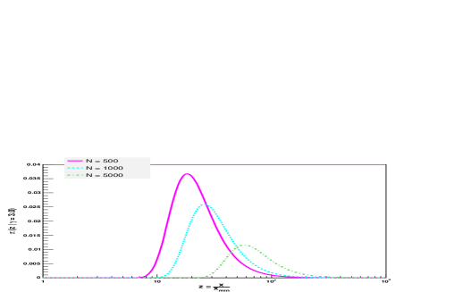
Figure 3: A plot of the probability distribution of the maximum of a sample drawn from a power-law with power index ${\gamma}=3.0$. This is the distribution $\pi(z)$ defined in equation (5) where $z$ is the ratio of the maximum to the minimum. The sample sizes are $N=500,\,1000$ and $5000$.

Motivated by the location and shape of $\pi(z)$ we consider the probability $P$ that the maximum ratio from a given sample $Z_{max}$ is less than or equal to a particular value , say $z$, in a convenient form as

$$P(Z_{max}\leq z)=\int_{1}^{z}\pi(t)dt\,=\,\left[1-z^{1-{\gamma}}\right]^{N}.$$ (6)

Indeed, with ${\gamma}=3.0$ (as in Fig. 3), $P(Z_{max}\leq 10)=6.6\times 10^{-3}$ for $N=500$, $4.3\times 10^{-5}$ for $N=1000$ and is $1.4\times 10^{-23}$ for $N=5000$. Another way to say this is that if one were to generate $10^{5}$ sets of events, each containing 1000 events drawn from a pure power-law with ${\gamma}=3.0$, $\sim 99.99\%$ of these sets would have a maximum element with a value greater than 10 times the minimum. For 500 events/set the fraction decreases to $\sim 99.34\%$. Such simulations were carried out in preparation for this note and the results were consistent with equation (6).

To apply this idea to the CR spectrum we consider the following null hypothesis: The flux of CR’s follow a power-law with index ${\hat{\gamma}}$ for all energies greater than a given minimum. As a test statistic for this hypothesis we use $P$, as defined in equation (6), with the interpretation that if the null hypothesis is true then $P$ is the probability that the ratio of the maximum energy to the minimum is less than or equal to the observed ratio. Typically, the null hypothesis is rejected at the 5% significance level (S.L.) if $P\leq 0.05$.

To calculate the value of $P$ for the observed data sets we need three pieces of information: the ratio of the maximum observed value to the minimum $z^{obs}_{max}$, the number of events $N_{tot}$ with values in the interval $[1,z_{max}]$ and a reasonable guess for the power index ${\gamma}$. Since a larger $z_{max}$ will lead to a larger value of $P$ we will conservatively take the highest energy AGASA (resp. Auger) event to fall on the upper edge of the highest energy bin. The method of determining the number of events in each bin is described in $\S$2 and here the parameter $N_{tot}$ represents the total number above a given minimum. We will use the logarithmically binned estimates and errors of ${\hat{\gamma}}$ discussed in $\S$2.

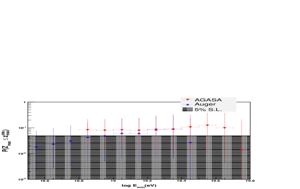
Figure 4: A plot of the probability that the maximum of a sample drawn from a power-law will be less than or equal to the maximum observed by the Auger ($E_{max}=10^{20}$, blue point-up) and AGASA ($E_{max}=10^{20.4}$, red point-down) experiments as a function of the minimum energy considered. The vertical error bars represent the effect of a $1\sigma_{{\hat{\gamma}}}$ deviation and the hatched area shows the 5% significance level.

The plot in Fig. 4 shows $P(Z_{max}\leq z^{obs}_{max})$ given $N_{tot}$ and ${\hat{\gamma}}$ as a function of minimum energy considered for each of the CR data sets in Fig. 2. In particular, for each $E_{min}$ the values of $N_{tot}$, $z^{obs}_{max}$ and ${\hat{\gamma}}\pm\sigma_{{\hat{\gamma}}}$ are estimated from the CR flux and the resulting $P$ are plotted for the Auger (blue) and AGASA (red) data. For example, the left-most Auger point represents the probability that if $N_{tot}=3567$ events are drawn from a power-law with ${\hat{\gamma}}=2.97^{+0.12}_{-0.12}$ then there is a $1.9^{+5.7}_{-1.6}\%$ chance that the maximum log-ratio $\log z_{max}$ would be less than or equal to that reported by the Auger experiment, namely $\log z^{obs}_{max}=\log 10^{20}/10^{18.5}$(eV). Taken at face value, one may reject the null hypothesis at the 5% S.L. for this data set. The left-most AGASA point represents the same probability for the complete set of AGASA data, namely $P(\log Z_{max}\leq\log 1.6)=8.4^{+13}_{-6.5}\%$ for $N_{tot}=1914$ events drawn from a power-law with ${\hat{\gamma}}=2.80^{+0.13}_{-0.13}$. Thus we cannot reject the null hypothesis for the AGASA data.

The upper (lower) vertical error bars depicted in Fig. 4 represent the value of $P$ if we have under (over) estimated the power index by $\sigma_{{\hat{\gamma}}}$, that is if ${\gamma}={\hat{\gamma}}\pm\sigma_{{\hat{\gamma}}}$, keeping the log-ratio and the total number of events constant. (The possible errors in the total number of events are on the order of a few percent and are negligible.) Since the fitting scheme considers successively lower energy bins, the points (and errors) for each experiment plotted in Fig. 4 are highly correlated. The upper error bars fall above the 5% S.L. for all minimums considered and therefore the statistical error associated with ${\hat{\gamma}}$ is enough to disallow rejection of the power-law hypothesis.

The biggest systematic measurement uncertainty in the CR data is the calibration of the energy. This uncertainty leads to an error in the reported absolute energy values of $\sim 30\%$ for the AGASA [8] data and as much as $\sim$50% for the highest energy events in the Auger data set. Since the probability considered here depends only on the ratio of the observed energies, it is independent of any constant systematic uncertainty in the energy determination. However, this probability is sensitive to energy errors which vary over the range considered and will thus cause uncertainty in $z^{obs}_{max}$.

For example, if we take the maximum to be 50% higher (but hold ${\hat{\gamma}}=2.97$ and $N_{tot}=3567$ constant) the value of $P$ represented by the left most Auger point in Fig. 4 changes from 1.9% to 17%. Thus the large uncertainty in $z^{obs}_{max}$ combined with the errors associated with ${\hat{\gamma}}$ implies that the preliminary Auger data set does not suggest sufficient evidence to reject the pure power-law hypothesis for all events above $E_{min}=10^{18.5}$(eV).

4 The TP-Statistic

Considering the error and extra degree of freedom associated with ${\gamma}$, an analysis of a distribution’s adherence to the power-law form without reference to, or regard for, this parameter is could lead to enhanced statistical power. First proposed by V. Pisarenko and D. Sornette , the so-called TP-statistic[12, 13] is a function of random variables that (in the limit of large $N$) tends to zero for samples drawn from a power-law, regardless of the value of ${\gamma}$. (TP stands for tail power, as oppossed to TE, also introduced in [12, 13], which stands for tail exponential.) This section will describe the TP-statistic and apply it to the CR data.

The raw moments of the pdf equation (1) are [1]

$$\langle z^{m}\rangle_{Z}=\int_{1}^{\infty}z^{m}f_{Z}(z)dz\rightarrow\begin{cases}\infty&m\geq{\gamma}\\ \frac{{\gamma}-1}{{\gamma}-1-m}&m<{\gamma}.\end{cases}$$ (7)

Thus power-laws with ${\gamma}\leq 3$ have a finite mean but an infinite variance (in the limit of large N) and sample statistics created from these moments are not particularly helpful. However, taking the natural logarithm of $z$ allows the integrals to converge and one may write (for all ${\gamma}>1$ and $m=0,1,2,\ldots$),

$$\nu_{m}=\langle\ln^{m}z\rangle_{Z}=\frac{m!}{({\gamma}-1)^{m}}.$$ (8)

The TP-statistic is calculated by noting that $\nu^{2}_{1}-\nu_{2}/2=0$. Therefore, if we use the sample analog of these quantities, namely

$${\hat{\nu}}_{m}=\frac{1}{N}\sum_{i=1}^{N}\ln^{m}\frac{x_{i}}{x_{min}}$$ (9)

then we can define (for all $x_{i}\geq u$),

$$TP(u)=\left(\frac{1}{N}\sum_{i=1}^{N}\ln\frac{x_{i}}{u}\right)^{2}-\frac{1}{2N}\sum_{i=1}^{N}\ln^{2}\frac{x_{i}}{u}.$$ (10)

By the law of large numbers this sample statistic tends to zero as $n\rightarrow\infty$, independent of the value of ${\gamma}$. The TP-statistic allows us to test for a power-law like distribution without comment about the value of the power index. Furthermore, for any one sample we can vary $u$ from the sample minimum $X_{min}$ to the sample maximum $X_{max}$ and calculate the TP-statistic over the range of $x$ in the sample.

Given complete event lists one may use equation (10) to calculate the TP-statistic for the unbinned data. Since only the binned CR flux is publicly available we adapt the statistic to a binned analysis and apply it first to an example distribution with a cutoff and then to the CR data sets.

4.1 An Example

In order to build intuition about the TP-statistic and its variance before studying the CR data, we first apply this statistic to simulated event sets drawn from both a pure power-law distribution and a similar distribution with a cut-off. The cut-off pdf is chosen so that it mimics a power-law for the lowest values but has an abrupt (and smooth) cut-off at a particular value, say $x_{cut}$. The functional form we will use here is

$$g(x)=B({\gamma},x_{min},x_{cut})\frac{x^{-{\gamma}}}{e^{x-x_{cut}}+1}.$$ (11)

The normalization of this pdf is $B({\gamma},x_{min},x_{cut})$, the value of which must be computed numerically. Fig. 5 contains a logarithmically binned histogram of 3000 events drawn from a pure power-law (black circles) with $x_{min}=1.0$ and ${\gamma}=3.0$, and two pdf’s in the from of equation (11); the magenta squares have $\log x_{cut}=1.0$ and the green triangles have $\log x_{cut}=1.5$. While arbitrary, the values of these parameters are chosen to be similar to the AGASA and Auger data (see Fig.1).

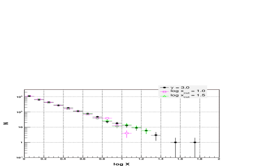
Figure 5: Logarithmically binned histogram of 3000 events drawn from a pure power-law with ${\gamma}=3.0$ and two power-laws with a cut, see equation (11). The magenta squares are drawn from the distribution with $\log x_{cut}=1.0$ and the green triangles have $\log x_{cut}=1.5$. As noted in the text, while arbitrary, the values of these parameters are chosen to be similar to the AGASA and Auger data (see Fig.1).

If we write the sorted (from least to greatest) values from a sample as $\{X_{(1)},$$X_{(2)},$ $\ldots\,,X_{(N)}\}$, the solid black line in Fig. 6 is created by calculating $TP(u=X_{(j)})$ for each value of the 3000 events drawn from the pure power-law histogram in Fig. 5. The circles represent the mean of the the statistic within the $i^{th}$ bin, say ${\overline{TP}}_{i}$, and the vertical error bars show the root-mean-squared deviation of the statistic within the bin. Note that the total number of events considered by the statistic decreases quickly from left to right which leads to a bias in and an increasing variance of the statistic.

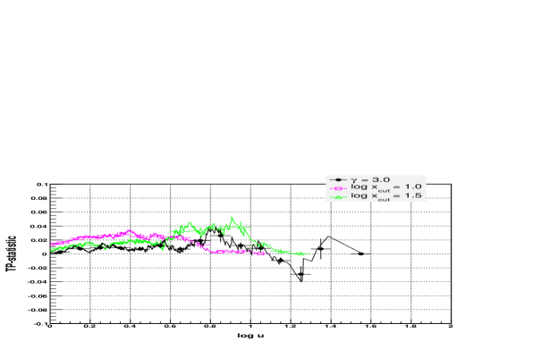
Figure 6: The TP-statistics, defined in equation equation (10), as a function of minimum value “$u$” for the 3 sets of 3000 events plotted in Fig. 5. Also plotted is the mean of the TP-statistic within each of the logarithmically spaced bins which is referred to in the text as ${\overline{TP}}$. The vertical error bars represent the RMS deviation of the statistic within each bin. Parenthetically, with increased statistics, say 10,000 events, the distinct characteristics of the TP-statistic for a pure power-law, a power-law with a cutoff $\log x_{cut}=1.0$ or a power-law with a cutoff $\log x_{cut}=1.5$ become more clearly different.

The jagged magenta line Fig. 6 shows the most obvious deviation from the power-law form; it is systematically offset from zero for nearly all minima of the data set. Of course, with 3000 events the histograms (see Fig. 5) are enough to distinguish between these two distributions. But the TP-statistic allows us to see this deviation by considering the entire data set (the left most magenta point in Fig. 6), not just by analyzing the events in the upper most bins. The green line in the figure shows $TP(u)$ for events drawn from equation (11) with $\log x_{cut}=1.5$. The histogram for this set is not as clearly different from the power-law as the magenta points and neither is the TP-statistic; the left-most green point shows no more deviation from zero than the power-law. However, as the minimum increases (and nears $x_{cut}$) the statistic moves away from zero (more noise not withstanding) and suggests that the data above the minimum deviate from the power-law.

It is important to note that the TP-statistic is positive for both of the cutoff distributions. Recall that for a pure power-law, $\nu^{2}_{1}-\nu_{2}/2=0$. The cutoff distribution, however, lacks an extended tail and will therefore have a smaller second log-moment $\nu_{2}$ as compared with (the square of) the first log-moment $\nu_{1}$ and will thus result in a positive TP-statistic. A distribution with an enhancement, rather than a cutoff, in the tail would result in a negative TP-statistic, since it would have a larger second log-moment (i.e. a larger “variance”). See the Appendix ($\S$6) for a detailed discussion of the TP-statistic applied to the double power-law.

To quantify the significance of the TP-statistics’ deviation from zero, $10^{4}$ sets of 3000 events were generated for each of the three distributions discussed in this section. For each set we calculate the mean TP-statistic ${\overline{TP}}$ within each of the logarithmically spaced bins. The resulting distribution of ${\overline{TP}}$’s within each bin is then fitted to a gaussian.

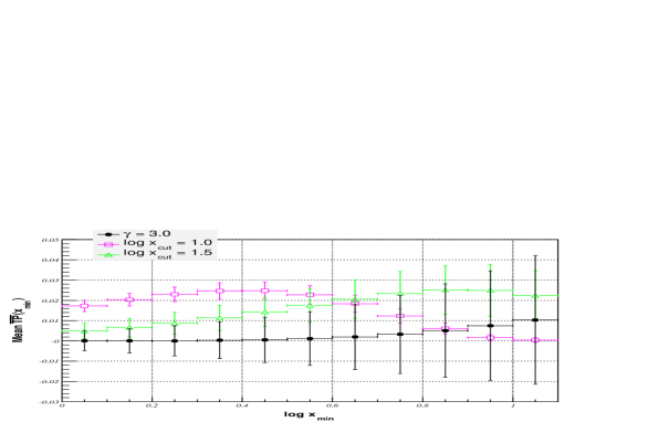
Figure 7: The fitted mean and $1\sigma$ deviation of the ${\overline{TP}}$’s (see definition in text) within each bin for the three distributions described in the text. This plot is the result of $10^{4}$ simulated sets of events, where Fig.6 is one example, and where each set contains 3000 events.

The black circles in Fig. 7 represent the mean of the gaussian fit to the distribution of ${\overline{TP}}$’s within each bin for a power-law and the error bars on the points represent the fitted $1\sigma$ deviation of the ${\overline{TP}}$’s. We interpret the left-most of these points in the following way: for 3000 events drawn from a power-law the “expected value” of ${\overline{TP}}$ in the first bin is effectively indistinguishable from zero, as expected.

Though the statistic itself does not depend on ${\gamma}$, the variance on this value does. The reason for this is that the variance of the ${\overline{TP}}$’s depends on the average total number of events greater than a given minimum, which is influenced by ${\gamma}$. In this case the total number of events per set for minima in the first bin is at least a few thousand and the variance of the ${\overline{TP}}$’s is $\sigma_{{\overline{TP}}}\sim 0.005$. These errors increase from left to right since each successively higher bin will contain ${\overline{TP}}$’s based on fewer and fewer events.

The magenta squares represent the fitted mean ${\overline{TP}}$ as a function of $x_{min}$ for sets drawn from a power-law with a cut-off at $\log x_{cut}=1.0$. They deviate from zero for all but the largest $x_{min}$. Furthermore, this offset is statistically significant for the lowest few bins of $x_{min}$, where the statistic reflects the deviation from power-law considering most of the events in the set. The green triangles show the fitted means for the $\log x_{cut}=1.5$ distribution. They also display some deviation from zero, but they are not as significant since they fall near the $1\sigma$ errors for the pure power-law distribution.

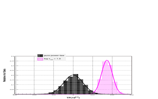
Figure 8: The distribution of the ${\overline{TP}}$’s in the first bin of Fig.7 (the bin with minimum $\log x_{min}=0.0$) for the simulated pure power-law (black, shaded) and a power-law with a cut-off at $\log x_{cut}=1.0$ (magenta, hatched). For these distributions $P_{TP}=0.00218$ (see equation (12)).

Indeed, one may inquire as to which of the bins deviate the most from the simulated power-law. This is equivalent to asking, “above what minimum do the data generated from this cut-off distribution maximally deviate from a pure power-law?” To quantify this deviation, we use a P-value given by

$$P_{TP}=1-\frac{1}{\sqrt{2\pi}}\int_{-\beta}^{\beta}e^{-t^{2}/2}dt,$$ (12)

where

$$\beta=\frac{|\mu_{1}-\mu_{2}|}{\sqrt{\sigma_{1}^{2}+\sigma_{2}^{2}}},$$ (13)

$\mu_{i}$ is the mean of the fitted gaussian and $\sigma_{i}$ is the standard deviation. We reject the pure power-law hypothesis (at the 5% S. L.) if $P_{TP}\leq 0.05$. The mean of the gaussian fit to the distribution of ${\overline{TP}}$’s for the power-law in the bin with minimum $\log x_{min}=0.0$ is $\mu_{1}=(0.0056\pm 5.1)\times 10^{-3}$ with a standard deviation $\sigma_{1}=4.9\times 10^{-3}$. The mean of the fitted gaussian for the $\log x_{cut}=1.0$ distribution in this bin is $\mu_{2}=(1.7\pm 0.28)\times 10^{-2}$ with a standard deviation $\sigma_{2}=2.8\times 10^{-3}$. Therefore, the significance level of the deviation is $P_{TP}=2.18\times 10^{-3}$ and we can reject the pure power-law hypothesis for this distribution. The distribution of the ${\overline{TP}}$’s for this bin is plotted in Fig. 8 for the pure power-law (black, shaded) and the $\log x_{cut}=1.0$ (magenta, hatched) pdf. The maximum deviation for the $\log x_{cut}=1.5$ pdf occurs in the bin with minimum $\log x_{min}=0.4$ and the corresponding distributions of ${\overline{TP}}$ are plotted in Fig. 9. The significance of this deviation is lower; $P_{TP}=0.298$.

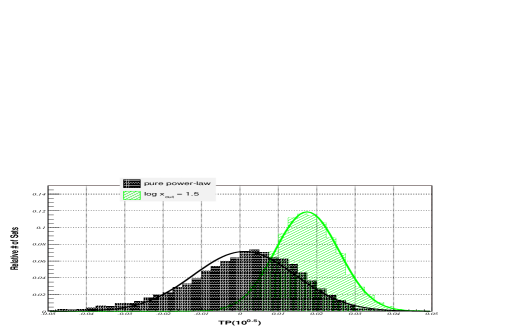
Figure 9: The distribution of the ${\overline{TP}}$’s in the fifth bin of Fig.7 (bin with minimum $\log x_{min}=0.4$) for the simulated pure power-law (black, shaded) and a power-law with a cut-off at $\log x_{cut}=1.5$ (green, hatched). For these distributions $P_{TP}=0.298$ (see equation (12)).

4.2 The Cosmic Ray Data

In order to apply the TP-statistic to the CR data, Monte-Carlo simulations were conducted and analyzed in a manner similar to that discussed in $\S$4.1; we generate $10^{4}$ sets of events from the reported flux and the resulting distribution of ${\overline{TP}}$ (within each bin) is fitted to a gaussian. Since the significance of deviation from zero depends on both the power index and the number of events, we will compare each of the Auger and AGASA data sets with a unique power-law. We will take the AGASA experiment to have $1916$ events above $\log E_{min}=18.8$ and we will compare the resulting TP-statistics with those of a power-law with the same minimum and ${\gamma}=2.80$. The Auger spectrum has a power-index estimate of $2.97$ considering all of the data above $\log E_{min}=18.5$ and a total of 3570 events, so we will therefore compare the TP-statistics arising from the Auger flux to those of a pure power-law with these parameters.

The application of this scheme to the AGASA spectrum is plotted in Fig. 10 in red triangles. The black circles represent average TP-statistic value for data drawn from a pure power-law with ${\hat{\gamma}}_{AGASA}$. Both plots have $N=886$ events per sky. The error bars on each point represent the 1-sigma deviation of the gaussian fit to the distribution of the mean TP-statistic. Since the AGASA values do not significantly deviate from zero (or the power-law values) this plot suggests that the AGASA distribution does not significantly deviate from a pure power-law. The most significant deviation occurs in the bin with minimum $10^{19.2}$(eV) and gives $P_{TP}=0.161$, which is consistent with the P-value for this bin discussed in $\S$3. These distributions are plotted in Fig 11.

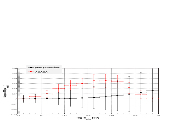
Figure 10: The fitted mean and $1\sigma$ deviation of the ${\overline{TP}}$’s (see definition on the text) within each bin for the AGASA spectrum (red triangles) and a pure power-law distribution (black circles). This plot is the result of $10^{4}$ simulated sets of events where each set contains 1916 events and the power-law has index ${\gamma}={\hat{\gamma}}_{AGASA}$.

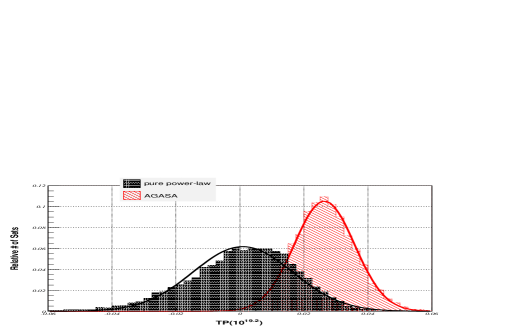
Figure 11: The distribution of ${\overline{TP}}$’s in the fifth bin of Fig.10 (the bin with minimum $E_{min}=10^{19.2}$(eV)) for the pure power-law (black, shaded) and the AGASA spectrum (red, hatched). For these distribution $P_{TP}=0.161$ (see equation (12)).

The simulation results from the Auger spectrum are plotted in Fig. 12. This plot shows deviation from a power-law for the lowest minimums considered. For the bin with minimum $\log E_{min}=18.6$ we find $P_{TP}=1.54\times 10^{-4}$. Thus we can say that the Auger spectrum with energies greater than $10^{18.6}$(eV) deviate from a power-law by $\sim 3.78\sigma$, where $\sigma^{2}=\sigma_{1}^{2}+\sigma_{2}^{2}$. The distribution of ${\overline{TP}}$’s for this minimum energy is plotted in Fig. 13.

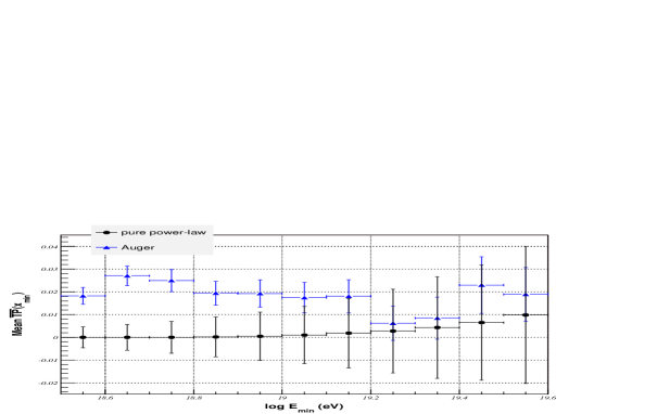
Figure 12: The fitted mean and $1\sigma$ deviation of the ${\overline{TP}}$’s (see definition on the text) within each bin for the Auger spectrum (blue triangles) and a pure power-law distribution (black circles). This plot is the result of $10^{4}$ simulated sets of events where each set contains 3570 events and the power-law has index ${\gamma}={\hat{\gamma}}_{Auger}$.

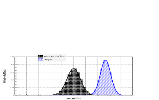
Figure 13: The distribution of ${\overline{TP}}$’s in the second bin of Fig.10 (the bin with minimum $E_{min}=10^{18.6}$(eV)) for the pure power-law (black, shaded) and the Auger spectrum (blue, hatched). For these distribution $P_{TP}=1.54\times 10^{-4}$ (see equation (12)).

Since the TP-statistic nearly eliminates the need to estimate ${\gamma}$, the biggest systematic uncertainty in analyzing the CR data with the TP-statistic is likely to be errors in the event energies. Similar to the $P$-value discussed in $\S$3, it is only the relative energy errors which can effect the result, since the TP-statistic depends only on the ratio. However, any elongation of the observed spectrum brought about by this relative uncertainty effect the TP-statistic. Without further study of the CR energy systematics, we cannot draw a conclusion from the $\sim 3.78\sigma$ deviation in Fig. 13.

5 Summary

In $\S$2 we use the reported (AGASA and Auger) CR fluxes to discuss the power-law form and illustrate the logarithmically binned estimates of the power index ${\gamma}$. The probability $P$ that the maximum value of a sample drawn from a power-law is less than or equal to a particular value is defined in equation (6). Using reasonable estimates for ${\gamma}$, $N_{tot}$ and $z^{obs}_{max}$ from the CR data sets we calculate $P$ in $\S$3. The value of $P$ is used to test the null hypothesis that these data sets follow a power-law . The AGASA data give no reason to reject the hypothesis; $P_{AGASA}\sim 8.4\%$ for the data with $\log E(eV)\geq 18.8$. The Auger data give more reason to reject the null hypothesis, $P_{Auger}\sim 1.9\%$ for the data with $\log E(eV)\geq 18.5$. However, consideration of the errors on ${\hat{\gamma}}$ prevent any solid conclusion.

For the purpose of statistical analysis it would be useful to eliminate, or at least minimize, the importance of ${\gamma}$. The TP-statistic tends (asymptotically) to zero regardless of the value of ${\gamma}$ and is the subject of $\S$4. We apply the TP-statistic to the CR data sets using a Monte-Carlo method described in $\S$4.2. The AGASA data give a value of $P_{TP}=0.161$ for energies greater than $10^{19.2}$(eV). a value consistent with the $P$-value discussed in $\S$3 (Fig.4). The preliminary Auger flux results in a TP-statistic with more significant deviation from the power-law form: $P_{TP}=1.54\times 10^{-4}$ for $E_{min}=10^{18.6}$(eV). Comparing this value with the $P$-value for this bin derived in $\S$3, namely $P\sim 2\times 10^{-2}$, illustrates the power of the method based on the TP-statistic which is essentially independent of gamma. Better understanding of the relative errors on the CR energies should lead to a definitive conclusion on the question of a cut-off in the CR spectrum.

6 Appendix

In $\S$4.1 we state that the TP-statistic will be distinctly positive for distributions which contain a tail-suppression and negative for distributions which contain a tail-enhancement (relative to the pure power-law form). In this section we numerically compute the TP-statistic for a “double power-law” distribution and describe the parameter space associated with this statistic.

Consider the following probability distribution function:

$$f(x)=\begin{cases}A(x_{min},x_{bend},{\gamma},\delta)x^{-{\gamma}}&x_{min}\leq x<x_{bend}\\ B(x_{min},x_{bend},{\gamma},\delta)x^{-\delta}&x_{bend}\leq x<\infty,\end{cases}$$ (14)

where $A(x_{min},x_{bend},{\gamma},\delta)$ and $B(x_{min},x_{bend},{\gamma},\delta)$ are chosen such that

$$\lim_{x\rightarrow x^{+}_{bend}}f(x)=\lim_{x\rightarrow x^{-}_{bend}}f(x)$$

and

$$\int_{x_{min}}^{\infty}f(x)dx=1.$$

This distribution follows a power-law with index ${\gamma}$ for $x_{min}\leq x<x_{bend}$, and $\delta$ for $x\geq x_{bend}$.

Given the parameter set $\{x_{min},x_{bend},{\gamma},\delta\}$, we define the TP-statistic for this distribution as

$$TP(u)=\left[\int_{u}^{\infty}\ln\left(\frac{x}{u}\right)f(x)dx\right]^{2}-\frac{1}{2}\int_{u}^{\infty}\ln^{2}\left(\frac{x}{u}\right)f(x)dx.$$ (15)

For $u\geq x_{bend}$ and/or ${\gamma}=\delta$ equation (15) is identically zero since it is equal to $\nu_{1}^{2}-1/2\nu_{2}$ (see equation (8)). However, equation (15) is non-trivial when $x_{min}\leq u<x_{bend}$ and ${\gamma}\neq\delta$. In what follows, we calculate $TP(u)$ for $x_{min}\leq u<x_{bend}$ and various values of $x_{bend}$ and $\delta$ with $x_{min}=1$ and ${\gamma}=3$ fixed.

Fig.14 contains a plot of $\log f(x)$ versus $\log x$ with $\delta={\gamma}\pm 1$ for several choices of $\log x_{bend}$ (namely, for $\log x_{bend}$ varying from 1 to 2 in steps of 0.2). The red curves correspond to ${\gamma}<\delta=4$ (tail-suppression) and the blue curves have ${\gamma}>\delta=2$ (tail-enhancement). The TP-statistic for each of these distributions is shown in Fig.15 as a function of $u$. Examination of Fig.15 suggests the following conclusions for a given ${\gamma}$ and $\delta$:

• $TP(u)$ is positive for all values of $u$ and $x_{bend}$ if and only if ${\gamma}<\delta$, and it is negative if and only if ${\gamma}>\delta$.

• For $x_{bend}$ much greater than $x_{min}$, $TP(u=x_{min})$ is approximately zero. Specifically, as $x_{bend}/x_{min}\rightarrow\infty$, $TP(x_{min})\rightarrow 0$.

• The location of the maximum deviation, say $u_{0}$ where

  $$\left(\frac{\partial}{\partial u}TP(u)\right)_{u=u_{0}}=0,$$ (16)

  is highly correlated with the location of the bend $x_{bend}$. Indeed, we have found that there is a linear relationship between $\log u_{0}$ and $\log x_{bend}$ and that this relationship is independent of whether ${\gamma}$ is less than or greater than $\delta$.

• The maximum deviation of the TP-statistic, i.e. $TP(u_{0})$, is independent of $\log x_{bend}$.

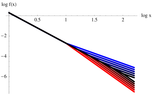
Figure 14: A plot of $\log f(x)$ (see equation (14)) versus $\log x$ with $\delta={\gamma}\pm 1$ for several choices of $\log x_{bend}$ (namely, for $\log x_{bend}$ varying from 1 to 2 in steps of 0.2). The red curves correspond to ${\gamma}<\delta=4$ (tail-suppression) and the blue curves have ${\gamma}>\delta=2$ (tail-enhancement). The more black the color of the curve, the larger $\log x_{bend}$.

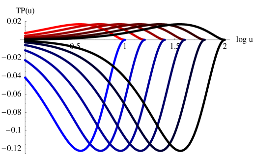
Figure 15: A plot of $TP(u)$ (see equation (15)) for each of the distributions plotted in Fig.14. Those distributions with tail-suppression (red) have $TP(u)>0$ and those with tail-enhancement (blue) have $TP(u)<0$.

To isolate the effects of power index choice, consider the family of distributions where $\log x_{bend}=1.0$ is fixed but $\delta$ is allowed to vary. Since the integrals in equation (15) only converge if $\delta\geq 2$, the minimum $\delta$ we can choose is $\delta=2$. There is no upper bound on $\delta$ so we vary this parameter over the interval $2\leq\delta<3$ in steps of 0.2 and over the interval $3<\delta<10$ in steps of 0.5. Fig.16 contains a plot of $\log f(x)$ versus $\log x$ with $\log x_{bend}=1.0$ and ${\gamma}=3$. The blue curves have $2\leq\delta<3$ (i.e. $\delta-{\gamma}<0$) and the red curves have $3<\delta<10$ (i.e. $\delta-{\gamma}>0$). The more black the color of these curves, the closer $\delta$ is to ${\gamma}$.

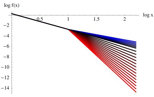
Figure 16: A plot of $\log f(x)$ (see equation (14)) versus $\log x$ with $\log x_{bend}=1.0$ and ${\gamma}=3$. The blue curves have $2\leq\delta<3$ (i.e. $\delta-{\gamma}<0$) and the red curves have $3<\delta<10$ (i.e. $\delta-{\gamma}>0$). The more black the color of these curves, the closer $\delta$ is to ${\gamma}$.

Fig.17 contains a plot of $TP(u)$ for the distributions plotted in Fig.16. As noted earlier, $TP(u)>0$ if and only if $\delta-{\gamma}>0$ and $TP(u)<0$ if and only if $\delta-{\gamma}<0$. The colored points on these curves show where each curve maximally deviates from zero; the coordinates of these points are $\{u_{0},TP(u_{0})\}$ for each curve (see equation (16)). These points show a weak dependence of $\log u_{0}$ on $\delta$, for a given $\log x_{bend}$.

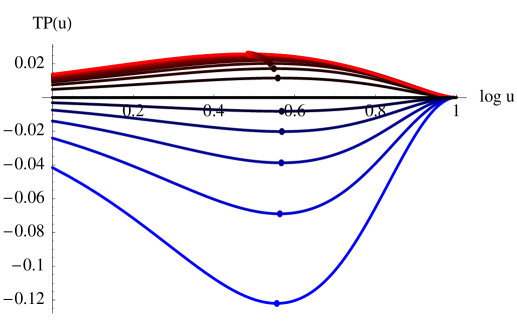
Figure 17: A plot of $TP(u)$ (see equation (15)) for the distributions plotted in Fig.16. The colored points on these curves show where each curve maximally deviates from zero; the coordinates of these points are $\{u_{0},TP(u_{0})\}$ for each curve (see equation (16)).

The value of the maximum deviation $TP(u_{0})$ also shows dependence on $\delta$. In Fig.18 we plot $TP(u_{0})$ versus $\delta-{\gamma}$ for each of the points in Fig.17. These plots suggest the following:

• For $-1\leq\delta-{\gamma}\lesssim 1$ (blue and black), a small change in $\delta$ will lead to a large change in $TP(u_{0})$.

• If $\delta-{\gamma}\gg 1$ (bright red), however, a large change in $\delta$ will result in a small change in $TP(u_{0})$. This case is of particular interest since a large $\delta$ will mimic the cutoff distribution defined in equation (11).

• By inspection of Fig.18 we note that $TP(u_{0})\approx 0.025$ for $\delta-{\gamma}\gg 1$.

• Comparison with Fig.15 suggests that the limiting value of $TP(u_{0})$ is roughly independent of $x_{bend}$.

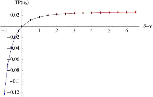
Figure 18: A plot of $TP(u_{0})$ (see equations (14) and (16)) versus $\delta-{\gamma}$ for each of the points in Fig.17. Note that $TP(u_{0})\approx 0.025$ for $\delta-{\gamma}\gg 1$.

The studies described in this section show that the TP-statistic can distinguish tail-suppressed ($\delta-{\gamma}>0$) from tail-enhanced ($\delta-{\gamma}<0$) distributions, i.e. $TP(u)>0$ if and only if $\delta-{\gamma}>0$ and $TP(u)<0$ if and only if $\delta-{\gamma}<0$. Furthermore, they show that in the limiting case of $\delta-{\gamma}\gg 1$ the most important parameter in determining $u_{0}$ is $x_{bend}$ but that the limiting value of $TP(u_{0})$ is roughly independent of $x_{bend}$ and $\delta-{\gamma}$.

References

- [1] M. E. J. Newman, Contemporary Physics 46, 323-351 (2005).
- [2] A. Clauset, M. Young and K.S. Gleditsch, arXiv:physics/0606007 (2006).
- [3] K. Greisen, Phys. Rev, Lett. 16, 748 (1966).
- [4] G.T. Zatsepin and V.A. Kuzmin, JETP. Lett. 4 78, (1966).
- [5] John N. Bachall and Eli Waxman arXiv:hep-ph/0206217 v5 (2003).
- [6] Auger Collaboration, Proceedings ICRC, Pune, India, 10 115 (2005), arXiv:astro-ph/0604114.
- [7] T. Yamamoto and The Pierre Auger Collaboration, arXiv:astro-ph/0601035 v1 (2006).
- [8] M. Takeda et al., Phys. Rev. Lett. 81 6 (1998).
- [9] Unbinned maximum likelihood methods have less error and bias when applied to power-law (or similar) distributions than binned methods[10]. They can also be modified to include energy error and variable acceptance information[11]. Lacking this information, we use the logarithmically binned estimate of where necessary. The minimum variance for any estimator of is given by the Cramer-Rao lower bound; .
- [10] M. L. Goldstein, S. A. Morris, and G. G. Yen, Eur. Phys. J. B. 41, 255-258 (2004).
- [11] L.W. Howell, Statistical Properties of Maximum Likelihood Estimators of Power Law Spectra Information, NASA/TP-2002-212020/REV1, Marshall Space Flight Center, Dec., 2002.
- [12] V. Pisarenko, D. Sornette and M Rodkin, Deviations of the Distributions of Seiesmic Energies from the Gutenberg-Richter Law, Computational Seismology 35, 138-159 (2004), arXiv:physics/0312020.
- [13] V. Pisarenko, D. Sornette, New Statistic for Financial Return Distributions: power-law or exponential?, arXiv:physics/0403075.