Magnetorotational collapse of massive stellar cores to neutron stars:
Simulations in full general relativity

Abstract

We study magnetohydrodynamic (MHD) effects arising in the collapse of magnetized, rotating, massive stellar cores to proto-neutron stars (PNSs). We perform axisymmetric numerical simulations in full general relativity with a hybrid equation of state. The formation and early evolution of a PNS are followed with a grid of $2500\times 2500$ zones, which provides better resolution than in previous (Newtonian) studies. We confirm that significant differential rotation results even when the rotation of the progenitor is initially uniform. Consequently, the magnetic field is amplified both by magnetic winding and the magnetorotational instability (MRI). Even if the magnetic energy $E_{\rm EM}$ is much smaller than the rotational kinetic energy $T_{\rm rot}$ at the time of PNS formation, the ratio $E_{\rm EM}/T_{\rm rot}$ increases to 0.1–0.2 by the magnetic winding. Following PNS formation, MHD outflows lead to losses of rest mass, energy, and angular momentum from the system. The earliest outflow is produced primarily by the increasing magnetic stress caused by magnetic winding. The MRI amplifies the poloidal field and increases the magnetic stress, causing further angular momentum transport and helping to drive the outflow. After the magnetic field saturates, a nearly stationary, collimated magnetic field forms near the rotation axis and a Blandford-Payne type outflow develops along the field lines. These outflows remove angular momentum from the PNS at a rate given by $\dot{J}\sim\eta E_{\rm EM}C_{B}$, where $\eta$ is a constant of order $\sim 0.1$ and $C_{B}$ is a typical ratio of poloidal to toroidal field strength. As a result, the rotation period quickly increases for a strongly magnetized PNS until the degree of differential rotation decreases. Our simulations suggest that rapidly rotating, magnetized PNSs may not give rise to rapidly rotating neutron stars.

I Introduction

The explosion mechanism in core-collapse supernovae has been pursued for several decades, but the problem has not yet been solved. Neutrino-driven convection has been suggested as a way of rejuvenating the stalled shock, while rotation and magnetic fields have also been proposed as key driving mechanisms (see e.g., WJ05 for a review). Recently, acoustic power generated by accretion-triggered g-mode oscillations of the proto-neutron star (PNS) has been offered as an explanation for the explosion OBDE06 .

Even if rotation and magnetic fields are not the main mechanisms, they may still have an important influence on a supernova explosion, especially when a long-soft gamma-ray burst is produced. In addition, several observations can be explained naturally by magnetic fields. For example, the rapid spindown of anomalous X-ray pulsars may result from the amplification of the star’s magnetic field during core collapse AXP ; TD . Soft gamma-ray repeaters AXP are likely to be neutron stars with very strong magnetic fields (so-called “magnetars”) DT .

It has been speculated that the magnetic field strength could be amplified to $\sim 10^{16}$ G during stellar core collapse, and the resulting strong magnetic field could play a crucial role in the supernova explosion WMW ; AHM ; TCQ ; TQB . The collapse is generically nonhomologous, with the inner core collapsing faster than the outer core. Thus, even if the progenitor has a rigid rotation profile at the onset of the collapse, differential rotation naturally develops with angular velocity decreasing outward. In the presence of such differential rotation, the magnetic field is amplified both by magnetic winding spitzer ; spruit ; BSS ; Shapiro and the magnetorotational (magneto-shear) instability (MRI) MRI0 ; MRI ; MRIrev . The field strength may thus grow by many orders of magnitude, even if it is initially small. The field amplification is likely to continue until the kinetic energy associated with the differential rotation $T_{\rm diff}$ is converted to magnetic energy $E_{\rm EM}$ Shapiro . Typically, $T_{\rm diff}$ is an appreciable fraction of the total rotational kinetic energy $T_{\rm rot}$. The amplified magnetic field results in a strong magnetic stress, which could blow off the matter in the vicinity of the PNS, converting magnetic energy back into matter kinetic energy and driving an outflow. The typical rotational kinetic energy of a PNS is approximately

$$T_{\rm rot} = {1\over 2}\kappa_{I}MR^{2}\Omega^{2}$$ (1)

$$= 4\times 10^{51}\biggl{(}{\kappa_{I}\over 0.3}\biggr{)}\biggl{(}{M\over 1.4M_{\odot}}\biggr{)}$$

$$~{}~{}~{}~{}~{}~{}\times\biggl{(}{R\over 10~{}{\rm km}}\biggr{)}^{2}\biggl{(}{P_{\rm rot}\over 2~{}{\rm ms}}\biggr{)}^{-2}~{}{\rm ergs},$$

where $M$, $R$, and $\Omega(=2\pi/P_{\rm rot})$ are the mass, radius, and angular velocity of the PNS, and $\kappa_{I}\sim$0.3–0.6 denotes the ratio of the moment of inertia to $MR^{2}$ and depends on the structure of the neutron star FIP ; CST . Thus, if the rotation period of the PNS is shorter than $\sim 4$ ms, and if a large fraction of the rotational kinetic energy is converted to the kinetic energy of the outward matter flow via magnetohydrodynamic (MHD) processes, the supernova explosion may be significantly powered by magnetorotational effects.

Numerical simulations of magnetorotational core collapse were pioneered by LeBlanc and Wilson LW and by Symbalisty Sym in the 1970s and 1980s, respectively. In the past few years (e.g., YS ; SKY ; TKNS ; Kotake ; OAM ; OADM ; ABM ; MBA ), this has become an active research topic in computational astrophysics. All of the simulations to date have been performed by assuming Newtonian gravitation or by including the general relativistic effects approximately OADM . Yamada and his collaborators have performed a variety of simulations in axial symmetry with simplified microphysics for a variety of rotational profiles and magnetic field strengths YS ; SKY . They found that the initially poloidal magnetic field is primarily amplified by compression during infall and by magnetic winding following core collapse. They also found that the magnetic pressure, which is amplified during collapse, could drive a strong outflow along the rotation axis. Their simulations were done in the nonuniform spherical polar coordinates $(r,\theta)$ with a grid size of at most (300, 50). At this resolution, they were not able to resolve the MRI. Takiwaki et al. TKNS performed simulations similar to those of Yamada et al., but with a realistic equation of state (EOS), and obtained essentially the same results. Kotake et al. Kotake performed a simulation adopting a strong toroidal magnetic field and an extremely high degree of differential rotation as the initial condition and found that the toroidal magnetic field can power the explosion for this special initial condition. Obergaulinger, Aloy, and Müller OAM performed similar simulations to those by Yamada et al. but with a slightly better grid resolution, (380, 60), in spherical polar coordinates. They indicated that not only magnetic winding but also the MRI could play an important role in the supernova explosion and evolution of the PNS. However, the grid resolution they adopted was also not sufficient for resolving the regions in which the MRI occurs most strongly OAM0 . Ardeljan, Bisnovatyi-Kogan, and Moiseenko ABM ; MBA performed axisymmetric simulations with a Lagrangian scheme. In their work, a purely hydrodynamic simulation was performed up to the formation of a PNS. Then they added a poloidal magnetic field to the PNS to study the MHD effects. They found that such effects, and, in particular the enhancement of the magnetic field strength by magnetic winding, could result in buoyancy and trigger a supernova explosion. They also reported that an MRI-like instability played an important role. However, in their simulation, the instability is observed only after $\sim 100P_{\rm rot}$, long after the toroidal field first becomes significant. But the fastest-growing mode for the (shear-type) MRI is amplified exponentially in a few rotation periods, irrespective of the strength of the toroidal fields MRIrev . Thus, the instability that they found is unlikely to be a shear-type instability spruit ; rather it is likely to be the magneto-convective instability (see discussion in Sec. VII).

All of these previous simulations have provided a qualitative picture of magnetorotational core collapse and supernova explosions. However, not all of the important magnetorotational effects have been incorporated in the simulations, mainly because of insufficient grid resolution. Hence, some fundamental questions concerning the magnetorotational explosion scenario have not been answered. For example, it has been established that the magnetic field is amplified during the collapse and during the subsequent evolution of the PNS, but what determines the saturated field strength and how large is it? How important are the effects of the MRI? Rotational kinetic energy of the PNS can be converted to outflow kinetic energy via MHD processes such as magnetic winding and the MRI. How efficiently is the rotational kinetic energy of the PNS converted to matter outflow energy? What is the rate of decrease of the rotational kinetic energy of the PNS and the corresponding rate of its period increase? After the magnetic field saturates, the magnetic configuration in the PNS will settle down to a stationary state. What is this final state? What mechanisms drive outflow?

Previous work has been performed mainly in the framework of Newtonian gravitation. However, general relativistic effects are not negligible and may have significant influence in the evolution of the PNS (particularly for a massive progenitor). Furthermore, after the collapse, shocks and outflows are often produced at relativistic speed. From a technical point of view, general relativistic simulations have an additional advantage. In the Newtonian case, the Alfvén velocity may exceed the speed of light (especially in the low-density region), and hence, the Courant condition for the time step can be quite severe. On the other hand, the Alfvén velocity is guaranteed to be smaller than the speed of light in general relativity, and so we do not have to deal with this unphysical complication.

In this paper, we summarize results from axisymmetric simulations in full general relativity using two general relativistic magnetohydrodynamical (GRMHD) codes independently developed recently DLSS ; SS05 ; DLSSS ; DLSSS2 . One purpose is to demonstrate that multi-dimensional MHD simulations for core collapse are now feasible in full general relativity, without approximation. The main purpose is to address the questions raised above by performing simulations with much higher grid resolution than those reported previously. We adopt a uniform grid in cylindrical coordinates so that we can achieve uniformly high resolution everywhere in our computation domain, and the MRI can be resolved wherever it occurs. We have also performed simulations using fisheye coordinates (see CLZ06 and Appendix A), which provides high resolution in the central region while using relatively few of grid points. As in previous works YS ; SKY ; OAM , we employ a simplified hybrid EOS since we want to focus on studying the MHD effects on the collapse and on the evolution of the magnetized PNS.

The latest study on supernova progenitors HWS suggests that magnetized, massive stars of solar metallicity may not be rotating as rapidly as the models we consider in this paper. It suggests that the typical value of $P_{\rm rot}$ at formation of a PNS is $\sim 15$ ms. The reason is that the magnetic field grows due to a dynamo mechanism during stellar evolution. As a result, angular momentum is transported outwards by magnetic braking, which decreases the rotation period in the central region of a massive star. If this scenario holds for all progenitors, the magnetorotational explosion scenario would not be effective since a substantial amount of rotational kinetic energy is required ($P_{\rm rot}\mathrel{\raise 1.29167pt\hbox{$<$}\mkern-14.0mu\lower 2.58334pt\hbox{$\sim$}}$ 5 ms), as shown in Eq. (1). However, the rotational kinetic energy of the supernova progenitor depends strongly on model parameters of the dynamo theory and there is still a possibility of forming a rapidly rotating progenitor if the progenitor is massive HWS . The magnetorotational scenario thus warrants detailed investigation. In this paper, we consider initial pre-collapse stars with substantial rotational kinetic energies.

The remainder of the paper is organized as follows. In Sec. II, we briefly review our mathematical formalism and numerical methods for our GRMHD simulations. In Sec. III, we provide a qualitative summary of the magnetorotational effects that could play important roles in the evolution of a differentially rotating PNS. Sections IV and V describe our initial models and computational setup, respectively. In Sec. VI, we present our numerical results, focusing on the evolution of the magnetic fields and of the newly formed PNS. Finally, we summarize our conclusions in Section VII. Throughout this paper, we adopt geometrical units in which $G=1=c$, where $G$ and $c$ denote the gravitational constant and speed of light, respectively. Cartesian coordinates are denoted by $x^{k}=(x,y,z)$. The coordinates are oriented so that the rotation axis is along the $z$-direction. We define the coordinate radius $r=\sqrt{x^{2}+y^{2}+z^{2}}$, cylindrical radius $\varpi=\sqrt{x^{2}+y^{2}}$, and azimuthal angle $\varphi=\tan^{-1}(y/x)$. Coordinate time is denoted by $t$. Greek indices $\mu,\nu,\cdots$ denote spacetime components ($x,y,z$, and $t$), small Latin indices $i,j,\cdots$ denote spatial components ($x,y$, and $z$), and capital Latin indices $I,J,\cdots$ denote the poloidal components ($\varpi$ and $z$).

II Formulation

II.1 Brief summary of methods

The formulation and numerical scheme for the present GRMHD simulations are the same as those we reported in DLSS ; SS05 , to which the reader may refer for details.

The fundamental variables for the metric evolution are the three-metric $\gamma_{ij}$ and extrinsic curvature $K_{ij}$. We adopt the Baumgarte-Shapiro-Shibata-Nakamura (BSSN) formalism SN ; gw3p2 ; BS ; POT ; bina2 to evolve the metric. In this formalism, the evolution variables are the conformal factor $\psi\equiv e^{\phi}\equiv\gamma^{1/12}$, the conformal 3-metric $\tilde{\gamma}_{ij}=e^{-4\phi}\gamma_{ij}$, three auxiliary functions $F_{i}\equiv\delta^{jk}\partial_{j}\tilde{\gamma}_{ik}$ (or $\tilde{\Gamma}^{i}\equiv-\tilde{\gamma}^{ij}{}_{,j}$), the trace of the extrinsic curvature $K$, and the tracefree part of the extrinsic curvature $\tilde{A}_{ij}\equiv e^{-4\phi}(K_{ij}-\gamma_{ij}K/3)$. Here, $\gamma={\rm det}(\gamma_{ij})$. The full metric $g_{\mu\nu}$ is related to the three-metric $\gamma_{\mu\nu}$ by $\gamma_{\mu\nu}=g_{\mu\nu}+n_{\mu}n_{\nu}$, where the future-directed, timelike unit vector $n^{\mu}$ normal to the time slice can be written in terms of the lapse $\alpha$ and shift $\beta^{i}$ as $n^{\mu}=\alpha^{-1}(1,-\beta^{i})$.

The Einstein equations are solved in Cartesian coordinates. We employ the Cartoon method cartoon ; shiba2d to impose axisymmetry. In addition, we also assume a reflection symmetry with respect to the equatorial plane and only evolve the region with $x>0$ and $z>0$. We perform simulations using a fixed uniform grid with size $N\times 3\times N$ in $x-y-z$ which, covering a computational domain $0\leq x\leq L$, $0\leq z\leq L$, and $-\Delta\leq y\leq\Delta$. Here, $N$ and $L$ are constants and $\Delta=L/N$. The variables in the $y=\pm\Delta$ planes are computed from the quantities in the $y=0$ plane by imposing axisymmetry.

The lapse $\alpha$ and shift $\beta^{i}$ are gauge functions that have to be specified in order to evolve the metric. In the code of SS05 , an approximate maximal slice (AMS) condition $K\approx 0$ is adopted following previous papers gw3p2 ; gr3d ; bina2 . In this condition, $\alpha$ is determined by solving approximately an elliptic-type equation. The shift is determined by the hyperbolic gauge condition as in S03 ; STU . In the code of DLSS , the lapse and shift are determined by hyperbolic driver conditions as in DSY04 .

The fundamental variables in ideal MHD are the rest-mass density $\rho$, specific internal energy $\varepsilon$, pressure $P$, four-velocity $u^{\mu}$, and magnetic field $b^{\mu}$ measured by an observer comoving with the fluid. The ideal MHD condition is written as $u_{\mu}F^{\mu\nu}=0$, where $F^{\mu\nu}$ is the electromagnetic tensor. The tensor $F^{\mu\nu}$ and its dual in the ideal MHD approximation are given by

$$F^{\mu\nu}=\epsilon^{\mu\nu\alpha\beta}u_{\alpha}b_{\beta},$$ (2)

$$F^{*}_{\mu\nu}\equiv{1\over 2}\epsilon_{\mu\nu\alpha\beta}F^{\alpha\beta}=b_{\mu}u_{\nu}-b_{\nu}u_{\mu},$$ (3)

where $\epsilon_{\mu\nu\alpha\beta}$ is the Levi-Civita tensor. The magnetic field measured by a normal observer $n^{\mu}$ is given by

$$B^{\mu}\equiv n_{\nu}F^{*\nu\mu}=\alpha(u^{t}b^{\mu}-b^{t}u^{\mu}),$$ (4)

From the definition of $B^{\mu}$ and the antisymmetry of $F^{\mu\nu}$ we have $n_{\mu}B^{\mu}=0=B^{t}$. The relations between $b^{\mu}$ and $B^{i}$ are

$$b^{t}={B^{j}u_{j}\over\alpha},$$ (5)

$$b^{i}={1\over\alpha u^{t}}\Big{(}B^{i}+B^{j}u_{j}u^{i}\Big{)}.$$ (6)

Using these variables, the energy-momentum tensor is written as

$$T_{\mu\nu}=T_{\mu\nu}^{\rm Fluid}+T_{\mu\nu}^{\rm EM},$$ (7)

where $T_{\mu\nu}^{\rm Fluid}$ and $T_{\mu\nu}^{\rm EM}$ denote the fluid and electromagnetic pieces of the stress-energy tensor. They are given by

$$T_{\mu\nu}^{\rm Fluid}=\rho hu_{\mu}u_{\nu}+Pg_{\mu\nu},$$ (8)

$$T_{\mu\nu}^{\rm EM}=F_{\mu\sigma}F^{~{}\sigma}_{\nu}-{1\over 4}g_{\mu\nu}F_{\alpha\beta}F^{\alpha\beta}$$

$$~{}~{}~{}~{}~{}~{}=\biggl{(}{1\over 2}g_{\mu\nu}+u_{\mu}u_{\nu}\biggr{)}b^{2}-b_{\mu}b_{\nu}.$$ (9)

Here, $h\equiv 1+\varepsilon+P/\rho$ is the specific enthalpy and $b^{2}\equiv b^{\mu}b_{\mu}$. Hence, the total stress-energy tensor becomes

$$T_{\mu\nu}=(\rho h+b^{2})u_{\mu}u_{\nu}+\left(P+\frac{b^{2}}{2}\right)g_{\mu\nu}-b_{\mu}b_{\nu}\ .$$ (10)

The quantity $b^{2}$ is often referred to as the magnetic energy density, and $b^{2}/2=P_{\rm mag}$ as the magnetic pressure.

In our numerical implementation of the GRMHD and magnetic induction equations, we evolve the weighted density $\rho_{*}$, weighted momentum density $S_{i}$, weighted energy density $S_{0}$, and weighted magnetic field ${\cal{B}}^{i}$. They are defined as

$$\rho_{*}\equiv-\sqrt{\gamma}\,\rho n_{\mu}u^{\mu},$$ (11)

$$S_{i}\equiv-\sqrt{\gamma}\,T_{\mu\nu}n^{\mu}\gamma^{\nu}_{~{}i},$$ (12)

$$S_{0}\equiv\sqrt{\gamma}\,T_{\mu\nu}n^{\mu}n^{\nu},$$ (13)

$${\cal{B}}^{i}\equiv\sqrt{\gamma}\,B^{i}.$$ (14)

During the evolution, we also need the three-velocity $v^{i}=u^{i}/u^{t}$.

The GRMHD and induction equations are written in conservative form for variables $\rho_{*}$, $S_{i}$, $S_{0}$, and ${\cal{B}}^{i}$ and evolved using a high-resolution shock-capturing scheme (HRSC). In the code of SS05 , the high-resolution central (HRC) kurganov-tadmor ; SFont scheme is employed. In this approach, the transport terms such as $\partial_{i}(\cdots)$ are computed by a Kurganov-Tadmor scheme with a third-order (piecewise parabolic) spatial interpolation. It has been demonstrated SFont that the results obtained using this scheme approximately agree with those using an HRSC scheme based on Roe-type reconstruction for the fluxes Font ; shiba2d . In the code of DLSS , the transport terms are evaluated by the HLL (Harten, Lax and van-Leer) flux formula HLL . The cell interface data reconstruction is done by the monotonized central (MC) scheme vL77 . It has also been demonstrated that the performance of the HLL scheme is as good as the Roe-type and HRC schemes in many MHD simulations valencia . The magnetic field ${\cal{B}}^{i}$ has to satisfy the no monopole constraint $\partial_{i}{\cal{B}}^{i}=0$. In the code of SS05 , this magnetic constraint is imposed by using the constrained transport scheme first developed by Evans and Hawley EH ; SS05 . In the code of DLSS , the flux-interpolated constrained transport (flux-CT) scheme t00 is employed. Both constrained transport schemes guarantee that no magnetic monopoles will be created in the computation grid during the numerical evolution. At each timestep, the primitive variables $(\rho,P,v^{i})$ must be computed from the evolution variables $(\rho_{*},S_{0},S_{i})$. This is done by numerically solving the algebraic equations (11)–(13) together with the EOS $P=P(\rho,\epsilon)$. As in many hydrodynamic simulations in astrophysics, we add a tenuous “atmosphere” that covers the computational grid outside the star. The atmospheric rest-mass density is set to $\approx 10^{-10}\rho_{c}(0)$ ($\approx 1~{}{\rm g/cm^{3}}$), where $\rho_{c}(0)$ is the initial central density of the star.

The codes used here have been tested in relativistic MHD simulations, including MHD shocks, nonlinear MHD wave propagation, magnetized Bondi accretion, MHD waves induced by linear gravitational waves, and magnetized accretion onto a neutron star. Furthermore, we have used both codes to perform simulations of the evolution of magnetized, differentially rotating, relativistic, hypermassive neutron stars, and obtain good agreement DLSSS ; DLSSS2 .

II.2 Equations of state

A parametric, hybrid EOS is adopted following Müller and his collaborators Newton4 ; HD ; OAM . In this EOS, the pressure consists of the sum of a cold part and a thermal part:

$$P(\rho,\epsilon)=P_{\rm P}(\rho)+P_{\rm th}(\rho,\epsilon).$$ (15)

The cold part of the pressure $P_{\rm P}$ depends only on the density. In this paper, we choose the following form of $P_{\rm P}$:

$$P_{\rm P}(\rho)=\left\{\begin{array}[]{ll}K_{1}\rho^{\Gamma_{1}},&\rho\leq\rho_{\rm nuc},\\ K_{2}\rho^{\Gamma_{2}},&\rho\geq\rho_{\rm nuc},\\ \end{array}\right.$$ (18)

where $K_{1}$, $K_{2}$, $\Gamma_{1}$ and $\Gamma_{2}$ are constants, and $\rho_{\rm nuc}\approx 2\times 10^{14}~{}\rm{g}/\rm{cm}^{3}$ is nuclear density. We set $K_{2}=K_{1}\rho_{\rm nuc}^{\Gamma_{1}-\Gamma_{2}}$ to make $P_{\rm P}$ continuous at $\rho=\rho_{\rm nuc}$. The adiabatic indices are chosen as $\Gamma_{1}$=1.3 or 1.32 and $\Gamma_{2}$=2.5 or 2.75. Following Newton4 ; HD , the value of $K_{1}$ is chosen to be $5\times 10^{14}$ in cgs units. With this choice, the cold part of the EOS for $\rho<\rho_{\rm nuc}$ is approximately given by relativistic degenerate electron pressure. This simplified cold EOS is designed to mimic a more complicated cold nuclear EOS. Using the first law of thermodynamics at zero temperature, we obtain the specific internal energy $\varepsilon_{\rm P}$ associated with the cold part of the pressure $P_{\rm P}$:

$$\varepsilon_{\rm P}(\rho) = -\int P_{\rm P}(\rho)\,d\left(\frac{1}{\rho}\right)$$ (19)

$$= \left\{\begin{array}[]{ll}\displaystyle{K_{1}\over\Gamma_{1}-1}\rho^{\Gamma_{1}-1},&\rho\leq\rho_{\rm nuc},\\ \displaystyle{K_{2}\over\Gamma_{2}-1}\rho^{\Gamma_{2}-1}+{(\Gamma_{2}-\Gamma_{1})K_{1}\rho_{\rm nuc}^{\Gamma_{1}-1}\over(\Gamma_{1}-1)(\Gamma_{2}-1)},&\rho\geq\rho_{\rm nuc}.\\ \end{array}\right.$$ (22)

The thermal part of the pressure $P_{\rm th}$ plays an important role when shocks occur. We adopt a simple form for $P_{\rm th}$:

$$P_{\rm th}=(\Gamma_{\rm th}-1)\rho\varepsilon_{\rm th},$$ (23)

where $\varepsilon_{\rm th}=\varepsilon-\varepsilon_{P}$ is the thermal specific internal energy. The value of $\Gamma_{\rm th}$ determines the efficiency of converting kinetic energy to thermal energy at shocks. We set $\Gamma_{\rm th}=\Gamma_{1}$ to conservatively account for shock heating.

II.3 Diagnostics

We monitor the total baryon rest mass $M_{*}$, ADM (Arnowitt-Deser-Misner) mass $M$, and angular momentum $J$, which are computed as in shiba2d ; DLSSS2 . We also compute the internal energy $E_{\rm int}$, thermal internal energy $E_{\rm heat}$, rotational kinetic energy $T_{\rm rot}$, gravitational potential energy $W$, and electromagnetic energy $E_{\rm EM}$ using the formulae given in DLSSS2 .

In a stationary, axisymmetric spacetime, the energy $E$ and angular momentum $J$ are conserved, where

$$E = \int\alpha\sqrt{\gamma}\,T^{t}_{~{}t}d^{3}x,$$ (24)

$$J = \int\alpha\sqrt{\gamma}\,T^{t}_{~{}\varphi}d^{3}x.$$ (25)

For a nearly stationary spacetime, which is achieved after the formation of the PNS, $E$ and $J$ are approximately conserved. We can then define the fluxes of rest mass, energy, and angular momentum across a sphere of coordinate radius $r$ by

$$F_{M}(r)=\oint_{r={\rm const}}dA\rho_{*}v^{r},$$ (26)

$$F_{E}(r)=-\oint_{r={\rm const}}dA\alpha\sqrt{\gamma}\,T^{r}_{~{}t},$$ (27)

$$F_{J}(r)=\oint_{r={\rm const}}dA\alpha\sqrt{\gamma}\,T^{r}_{~{}\varphi},$$ (28)

where $dA=r^{2}\sin\theta d\theta d\phi$. The energy and angular momentum fluxes associated with the electromagnetic fields are defined as

$$F_{E,{\rm EM}}(r)=-\oint_{r={\rm const}}dA\alpha\sqrt{\gamma}\,T^{\rm EM}{}^{r}_{~{}t},$$ (29)

$$F_{J,{\rm EM}}(r)=\oint_{r={\rm const}}dA\alpha\sqrt{\gamma}\,T^{\rm EM}{}^{r}_{~{}\varphi}.$$ (30)

The total energy flux $F_{E}$ is very close to the rest-mass flux $F_{M}$ since $F_{E}$ is primarily composed of the rest-mass energy flow. Thus, we define another energy flux by subtracting the rest-mass flow: $F_{e}=F_{E}-F_{M}$. We note that $F_{e}$ contains kinetic, thermal, electromagnetic, and gravitational potential energy fluxes. If $F_{e}>0$ at sufficiently large radius, an unbound outflow (overcoming gravitational binding energy) is present.

It should be noted that even in a stationary spacetime, one can choose gauges such that $\partial/\partial t$ is not a Killing vector. In this case, the energy $E$ defined above is not conserved. Thus, these are physical meaningful fluxes only in certain gauges. In our evolution, we find that after the formation of the PNS, the system relaxes to a stationary state and the metric does not change significantly with coordinate time $t$, suggesting that $\partial/\partial t$ is an approximate Killing vector in our simulations. Hence we use the above formulae to compute the fluxes.

II.4 Gravitational waveforms in terms of quadrupole formula

We compute gravitational waves in terms of the quadrupole formula given by SS ; SS04a :

$$h_{ij}=P_{i}^{~{}k}P_{j}^{~{}l}\biggl{(}{2\over r}{d^{2}\hbox{$\,I\!\!\!$--}_{kl}\over dt^{2}}\biggr{)},$$ (31)

where $\hbox{$\,I\!\!\!$--}_{ij}$ and $P_{i}^{~{}j}=\delta_{ij}-\hat{n}_{i}\hat{n}_{j}$ ($\hat{n}_{i}=x^{i}/r$) denote the tracefree quadrupole moment and the TT projection tensor, respectively. From this expression, the $+$-mode of quadrupole gravitational waves in an axisymmetric spacetime can be written as

$$h_{+}^{\rm quad}={\ddot{I}_{xx}(t_{\rm ret})-\ddot{I}_{zz}(t_{\rm ret})\over r}\sin^{2}\theta,$$ (32)

where $I_{ij}$ denotes the quadrupole moment, $\ddot{I}_{ij}$ is its second time derivative, $\theta$ denotes the angle between the rotation axis and the direction of observation, and $t_{\rm ret}$ is retarded time $t_{\rm ret}\approx t-r$. In this paper, we characterize the gravitational waves by the variable $A_{2}(t)\equiv\ddot{I}_{xx}(t_{\rm ret})-\ddot{I}_{zz}(t_{\rm ret})$, which has dimensions of length. In terms of $A_{2}$, the observed gravitational-wave strain is given by

$$h=1\times 10^{-20}\biggl{(}{A_{2}\over 3.1~{}{\rm m}}\biggr{)}\biggl{(}{10~{}{\rm kpc}\over r}\biggr{)}\sin^{2}\theta.$$ (33)

In spacetimes with strong gravitational fields, there is no unique definition for the quadrupole moment. Here, we choose for simplicity

$$I_{ij}=\int\rho_{*}x^{i}x^{j}d^{3}x.$$ (34)

Using the continuity equation, we compute the first time derivative as

$$\dot{I}_{ij}=\int\rho_{*}(v^{i}x^{j}+x^{i}v^{j})d^{3}x.$$ (35)

We then compute $\ddot{I}_{ij}$ by finite differencing the numerical values of $\dot{I}_{ij}$ in time.

Because of the ambiguity in the definition of the quadrupole moment in a spacetime with strong gravitational fields, one may choose alternative expressions for $I_{ij}$. Hence, the gravitational waveforms determined from the quadrupole formula depend on the chosen definition of $I_{ij}$. In addition, they depend on the gauge conditions, since the coordinates $r$ and $t$ appeared in $I_{ij}$ and $\dot{I}_{ij}$ are gauge dependent. We have calibrated our quadrupole formula in SS , and found that the magnitude of the error in the amplitude of gravitational waves is of order $M/R$, where $M$ and $R$ denote the typical mass and radius of the emitter. On the other hand, the phase of the waveforms is quite accurate. Thus, the wave amplitudes shown in this paper are not accurate to better than $\sim$10%, but the computed radiation possesses the correct qualitative features.

We also note that in our formula, the contribution from $T_{\mu\nu}^{\rm EM}$ is neglected. This is justified in the present treatment, since the contribution from the electromagnetic part is about 10% of the matter part, and hence, the error in neglecting the former is as large as the error of our quadrupole formula.

III Magnetorotational effects

In this section, we summarize processes that play an important role in magnetorotational core collapse and the subsequent evolution of the PNS.

III.1 Compression and magnetic winding during collapse

The magnetic field is amplified by compression and magnetic winding during stellar collapse. This can be understood by considering the magnetic induction equation in a perfectly conducting (ideal MHD) plasma:

$$\partial_{t}{\cal{B}}^{i}+\partial_{j}(v^{j}{\cal{B}}^{i}-v^{i}{\cal{B}}^{j})=0.$$ (36)

Combining Eq. (36) with the continuity equation

$${d\rho_{*}\over dt}+{\rho_{*}\over\varpi}\partial_{I}(\varpi v^{I})=0,$$ (37)

we rewrite the induction equation as

$${d{\cal{H}}^{I}\over dt}={\cal{H}}^{J}\partial_{J}v^{I},$$ (38)

$${d{\cal{H}}^{\varphi}\over dt}={\cal{H}}^{J}\partial_{J}\Omega,$$ (39)

where ${\cal{H}}^{i}\equiv{\cal{B}}^{i}/\rho_{*}$, $v^{\varphi}=\Omega$, and

$${d\over dt}\equiv{\partial\over\partial t}+v^{I}{\partial\over\partial x^{I}}.$$ (40)

For a pre-collapse star having moderate angular momentum, the core collapses in an approximately spherical and homologous manner. Hence $v^{r}\propto r$, which implies $v^{\varpi}\propto\varpi$, $v^{z}\propto z$, and $|v^{\varpi}|\approx|v^{z}|$. It follows from the continuity equation that

$${d\rho_{*}\over dt}\approx-3\rho_{*}{v^{\varpi}\over\varpi}.$$ (41)

Note that $v^{\varpi}$ and $v^{z}$ are negative. Combining the above equation with Eq. (38), we obtain

$${d{\cal{H}}^{\varpi}\over dt}\approx{\cal{H}}^{\varpi}{v^{\varpi}\over\varpi}\sim-{{\cal{H}}^{\varpi}\over 3}{d\ln\rho_{*}\over dt},$$ (42)

$${d{\cal{H}}^{z}\over dt}\approx{\cal{H}}^{z}{v^{\varpi}\over\varpi}\sim-{{\cal{H}}^{z}\over 3}{d\ln\rho_{*}\over dt}.$$ (43)

Hence for an observer comoving with the fluid,

$${\cal{H}}^{I}\propto\rho_{*}^{-1/3}\sim\rho^{-1/3},$$ (44)

which means that the poloidal field $B^{I}\propto\rho^{2/3}$ during core collapse.

While the collapse proceeds roughly homologously in the bulk of the star, this is not the case in the outer layers. Thus, significant differential rotation develops in the outer layers. We see from Eq. (39) that toroidal magnetic fields are amplified when there is differential rotation along the poloidal field lines (magnetic winding). The toroidal field is thus expected to grow during the collapse. However, since the growth depends on the non-homologous nature of the collapse in the outer layers, a simple prediction for the dependence of ${\cal{H}}^{\varphi}$ on $\rho$ [as in Eq. (44)] is not available.

To obtain a rough idea of how the toroidal field evolves during the collapse, we proceed as follows. Assume that $\Omega$ in the differentially rotating outer regions is described by $\varpi^{-p}$, where $p$ is constant with time. This will not apply in regions where the homology is seriously violated. However, the true behavior of $\Omega$ in the region of interest is not known analytically, and we are only seeking a rough estimate. Equation (39) gives

$${d{\cal{H}}^{\varphi}\over dt}\approx-p{{\cal{H}}^{\varpi}\Omega\over\varpi}.$$ (45)

The evolution of ${\cal{H}}^{\varphi}$ measured by the comoving observer is given by

$${\cal{H}}^{\varphi}\approx-\int dt\,p{{\cal{H}}^{\varpi}\Omega\over\varpi}.$$ (46)

For a comoving observer, $\varpi^{-1}\propto\rho^{1/3}$ and hence ${\cal{H}}^{\varpi}/\varpi$ is approximately constant according to Eq. (44). (This again assumes homologous collapse, which does not strictly hold in the regions of interest for the toroidal field growth.) When the magnetic field is weak and the spacetime is axisymmetric, the specific angular momentum of a fluid particle $j=hu_{\varphi}\approx\Omega\varpi^{2}$ is approximately conserved, which implies $\Omega\propto\varpi^{-2}\propto\rho^{2/3}$. We then have

$${\cal{H}}^{\varphi}\propto\int\Omega dt\propto\int\rho^{3/2}dt.$$ (47)

Next, we obtain an approximate relation between $dt$ and $d\rho$ from the following Newtonian analysis. Since the collapse is approximately spherical and homologous, conservation of energy implies

$$\frac{1}{2}v^{2}-\frac{m(r)}{r}=-\frac{m(r_{0})}{r_{0}},$$ (48)

where $r_{0}$ is the radius of the fluid particle at the onset of collapse ($t=0$). The mass interior to the radius $r$, $m(r)=m(r_{0})=(4\pi/3)r_{0}^{3}\rho_{0}$ is independent of time during homologous collapse. Here $\rho_{0}$ is the density of the fluid particle at $t=0$. Setting $v=-dr/dt$, we have

$$\frac{dr}{dt}=-\sqrt{m(r_{0})\left(\frac{1}{r}-\frac{1}{r_{0}}\right)}.$$ (49)

Combining the above equation with $\rho=\rho_{0}(r_{0}/r)^{3}$, we obtain

$$dt\propto\rho_{0}^{-1/2}\frac{d\rho/\rho_{0}}{(\rho/\rho_{0})^{4/3}\sqrt{(\rho/\rho_{0})^{1/3}-1}}.$$ (50)

Substituting Eq. (50) into Eq. (47), we have ${\cal{H}}^{\varphi}\propto\sqrt{(\rho/\rho_{0})^{1/3}-1}$, and hence we provide the following estimate of the toroidal field during the collapse:

$$B^{\varphi}\propto\rho\ \sqrt{\left(\frac{\rho}{\rho_{0}}\right)^{1/3}-1}\ .$$ (51)

When $\rho\gg\rho_{0}$, the above equation simplifies to

$${\cal{H}}^{\varphi}\propto\rho^{1/6}~{}~{}{\rm and}~{}~{}B^{\varphi}\propto\rho^{7/6}.$$ (52)

In practice, we find that $B^{\varphi}\propto\rho^{q}$, where $q$ is slightly less than 1. However, with the assumptions that went into Eq. (52), only rough agreement is to be expected.

III.2 PNS magnetic winding

When the central density of the collapsing star exceeds the nuclear density, the core bounces due to the stiff nuclear EOS. The star quickly settles down to a quasistationary state and a PNS is formed. In this quasistationary state, the toroidal magnetic field grows linearly with time. This can be seen from the induction equation (36). If the magnetic field is weak and has a negligible back-reaction on the fluid, the velocities will remain constant with time. In cylindrical coordinates, we have (assuming axial symmetry)

$$\partial_{t}{\cal{B}}^{I}\approx 0,$$ (53)

$$\partial_{t}{\cal{B}}^{\varphi}\approx{1\over\varpi}\partial_{I}(\varpi\Omega{\cal{B}}^{I}),$$ (54)

where we have assumed that $|v^{\varpi}|\ll\varpi\Omega$ and $|v^{z}|\ll\varpi\Omega$ when the PNS is in quasiequilibrium. Then,

$$\partial_{t}{\cal{B}}^{\varphi}\approx{\cal{B}}^{I}\partial_{I}\Omega,$$ (55)

where we used the no-monopole constraint [$\partial_{I}(\varpi{\cal{B}}^{I})=0$ in axisymmetry]. During the early phase of the PNS evolution, Eq. (55) indicates that the toroidal component of the field ${\cal{B}}^{T}(=\varpi{\cal{B}}^{\varphi})$ grows linearly according to

$$|{\cal{B}}^{T}(t;\varpi,z)|$$

$$\approx|{\cal{B}}^{T}(t_{p};\varpi,z)|+t\varpi|{\cal{B}}^{I}(t_{p};\varpi,z)\partial_{I}\Omega(t_{p};\varpi,z)|$$ (56)

$$\approx|{\cal{B}}^{T}(t_{p};\varpi,z)|+{3\pi t\over P_{\rm rot}}|{\cal{B}}^{\varpi}(t_{p};\varpi,z)|$$

$$=|{\cal{B}}^{T}(t_{p};\varpi,z)|$$

$$+10^{15}\biggl{(}{t\over 100~{}{\rm ms}}\biggr{)}\biggl{(}{P_{\rm rot}\over 1~{}{\rm ms}}\biggr{)}^{-1}\biggl{(}{|{\cal{B}}^{\varpi}(t_{p};\varpi,z)|\over 10^{12}~{}{\rm G}}\biggr{)}~{}{\rm G},$$ (57)

where $t_{p}$ is the time at which the PNS first settles down to a quasiequilibrium state, $P_{\rm rot}$ denotes the local rotation period, and we have assumed a Keplerian angular velocity profile $\Omega\propto\varpi^{-3/2}$. The growth of $B^{T}$ is expected to deviate from this linear relation when the magnetic tension is large enough to change the angular velocity profile of the fluid (magnetic braking). Magnetic braking transports angular momentum on the Alfvén timescale spitzer ; spruit ; BSS ; Shapiro :

$$t_{A} \sim \frac{R}{v_{A}}\approx 10~{}{\rm ms}\left(\frac{|{\cal{B}}^{\varpi}|}{10^{15}~{}{\rm G}}\right)^{-1}$$ (58)

$$~{}~{}~{}~{}~{}~{}~{}~{}~{}\times\left(\frac{R}{10~{}{\rm km}}\right)\left(\frac{\rho}{10^{14}~{}{\rm g/cm^{3}}}\right)^{1/2}\ ,$$

where $R$ is the characteristic radius of the PNS and $v_{A}\approx|B|/\rho^{1/2}$ is the Alfvén speed. So Eq. (57) holds for $t_{p}\lesssim t\lesssim t_{p}+t_{A}$.

III.3 Magnetorotational (shear) instability

The MRI is present in a weakly magnetized, rotating fluid wherever $\partial_{\varpi}\Omega<0$ MRI0 ; MRI ; MRIrev . When the instability reaches the nonlinear regime, the distortions in the magnetic field lines and velocity field lead to turbulence. To estimate the growth time scale $t_{\rm MRI}$ and the wavelength of the fastest-growing mode $\lambda_{\rm max}$, we can use a Newtonian local linear analysis given in MRIrev . Linearizing the MHD equations for a local patch of a rotating fluid and imposing a plane-wave dependence ($e^{i({\bf k}\cdot{\bf x}-\omega t)}$) on the perturbations leads to the dispersion relation given in Eq. (125) of MRIrev . Specializing this equation for a constant-entropy medium leads to the dispersion relation

$$\omega^{4}-[2({\bf k}\cdot{\bf v}_{A})^{2}+\kappa^{2}]\omega^{2}$$

$$~{}~{}~{}~{}~{}+({\bf k}\cdot{\bf v}_{A})^{2}[({\bf k}\cdot{\bf v}_{A})^{2}+\kappa^{2}-4\Omega^{2}]=0\ ,$$ (59)

where ${\bf v}_{A}={\bf B}/\sqrt{\rho}$ is the (Newtonian) Alfvén velocity vector and $\kappa$ is the epicyclic frequency of Newtonian theory:

$$\kappa^{2}\equiv\frac{1}{\varpi^{3}}\frac{\partial(\varpi^{4}\Omega^{2})}{\partial\varpi}.$$ (60)

Equation (59) is modified for a medium of inhomogeneous entropy MRIrev . In this section, we neglect any entropy gradients and focus on the effects of shear. We further simplify the analysis by considering only the vertical modes (${\bf k}=k{\bf e}_{z}$) since these are likely to be the dominant modes. The value of $\omega^{2}$ can be found by solving Eq. (59) and then minimized to obtain the frequency of the fastest-growing mode, $\omega_{\rm max}$:

$$\omega^{2}_{\rm max}=-\frac{1}{4}\left(\frac{\partial\Omega}{\partial\ln\varpi}\right)^{2}.$$ (61)

This maximum growth rate corresponds to

$$(kv_{A}^{z})^{2}_{\max}=\Omega^{2}-{\kappa^{4}\over 16\Omega^{2}}.$$ (62)

The growth time ($e$-folding time) and wavelength of the fastest-growing mode are then given by

$$t_{\rm MRI} = 1/(i\omega_{\rm max})=2\left|\partial\Omega/\partial\ln\varpi\right|^{-1}\ ,$$ (63)

$$\lambda_{\rm max} = \frac{2\pi}{k_{\rm max}}={2\pi v_{A}^{z}\over\Omega}\biggl{[}1-\biggr{(}{\kappa\over 2\Omega}\biggr{)}^{4}\biggr{]}^{-1/2}.$$ (64)

For a Keplerian angular velocity distribution $\Omega\propto\varpi^{-3/2}$, we have

$$t_{\rm MRI} = {4\over 3\Omega}\approx 1.3~{}{\rm ms}\ \left(\frac{\Omega}{1000~{}{\rm rad~{}s}^{-1}}\right)^{-1},$$ (65)

$$\lambda_{\rm max} = {8\pi v_{A}^{z}\over\sqrt{15}\Omega}$$ (66)

$$\approx 2.1~{}{\rm km}\ \left(\frac{\Omega}{1000~{}{\rm rad~{}s}^{-1}}\right)^{-1}$$

$$~{}~{}~{}~{}~{}~{}~{}\times\left(\frac{B^{z}}{10^{14}\ {\rm G}}\right)\left(\frac{\rho}{10^{13}~{}{\rm g/cm^{3}}}\right)^{-1/2}.\ \$$

If $B^{z}$ is comparable to the field strength of a canonical pulsar ($B^{z}\sim 10^{12}$ G), $\lambda_{\rm max}$ is much smaller than the typical radius $R$ of a PNS. Since $\lambda_{\rm max}\propto v_{A}$, larger magnetic fields will result in longer MRI wavelengths. When $\lambda_{\rm max}\mathrel{\raise 1.29167pt\hbox{$>$}\mkern-14.0mu\lower 2.58334pt\hbox{$\sim$}}100$ km, the MRI will be suppressed since the unstable perturbations will no longer fit inside the region with a high degree of differential rotation. Hence the MRI is regarded as a weak-field instability. In this paper, the initial magnetic field strength is chosen so that the field strength in the resulting PNS is $\sim 10^{14}$ G, giving $\lambda_{\rm max}\sim$ a few km.

Unlike $\lambda_{\rm max}$, $t_{\rm MRI}$ does not depend on the magnetic field strength but on the angular velocity profile. The Newtonian local analysis indicates that the MRI always grows on the timescale of a rotation period for a configuration with $\partial\ln\Omega/\partial\ln\varpi\sim-1$. Hence, the MRI is expected to play an important role for a PNS, especially near its surface, which is in general differentially rotating. The resulting strong magnetic fields and turbulence tend to transport angular momentum from the rapidly rotating inner region of the PNS to the more slowly rotating outer layers. This causes the inner part to contract and the outer layers to expand. We note, however, that once the magnetic field strength is saturated, the resulting angular momentum transport and matter outflow will be governed by the turbulence and is thus expected to occur on a time scale longer than $t_{\rm MRI}$ (e.g., a turbulent transport time scale).

III.4 MHD outflow by the magneto-spring effect

After the formation of the PNS, MHD outflows may transport angular momentum outward (causing a spindown of the PNS) and may power a supernova explosion WMW ; AHM . In the early stage of the evolution of the PNS, the MHD outflow may be driven by the toroidal magnetic field, which grows linearly due to magnetic winding according to Eq. (57). A helical magnetic field forms as a result. The rate of change of the magnetic energy associated with the toroidal field is

$$\dot{E}_{\rm EM} \sim{d(B^{T})^{2}\over dt}=2B^{T}\dot{B}^{T}$$ (67)

$$\approx 2B^{T}B^{\varpi}\varpi\partial_{\varpi}\Omega\approx-3B^{T}B^{\varpi}\Omega,$$

where we have assumed a Keplerian angular velocity profile $\Omega\propto\varpi^{-3/2}$. We note that $B^{T}B^{\varpi}$ should be negative [see Eqs. (39) and (55)]. Because of the growing magnetic pressure and hoop stress, material is lifted from the PNS along the rotation axis, producing a tower-like MHD outflow (see e.g., US ; KHM ; RUKL ).

If a significant amount of energy gained from magnetic winding is used to drive the MHD outflow, the rate of energy loss from the PNS is approximately

$$\dot{E}\sim E_{\rm EM}\Big{|}{B^{\varpi}\over B^{T}}\Big{|}\Omega,$$ (68)

where we have assumed that the magnetic energy is dominated by the toroidal field $B^{T}$. This process is likely to be important only in the early stage before the toroidal field saturates.

III.5 MHD outflow by magneto-centrifugal effect

Another type of MHD outflow may occur in a differentially rotating object penetrated both by poloidal and toroidal field lines. Blandford and Payne showed that when a stationary disk is penetrated by open magnetic fields and when a mechanism for matter ejection operates at the disk surface, a stationary magneto-centrifugal outflow is launched BP ; AHM (see also relevant computational work, e.g., BP1 ; BP2 ).

We first consider the magneto-centrifugal effect operating on an accretion disk. To estimate the order of magnitude of the energy flux in the outflow, we evaluate the Poynting flux approximately. We assume that the disk rotates with an angular velocity $\Omega_{d}$ and that the poloidal velocity is smaller than the rotational velocity. The Poynting flux along the poloidal field line is $\sim|\mbox{\boldmath$E$}\times\mbox{\boldmath$B$}|\sim R_{d}\Omega_{d}B^{P}B^{T}$, where $R_{d}$ is the characteristic radius of the disk, $B^{P}\sim B^{\varpi}$ is the magnitude of the poloidal magnetic field, and the electric field $E$ is calculated by the (Newtonian) ideal MHD condition $|\mbox{\boldmath$E$}|=|\mbox{\boldmath$v$}\times\mbox{\boldmath$B$}|\sim R_{d}\Omega_{d}B^{P}$. The energy generation rate is then given by

$$\dot{E}_{\rm Poyn} = ({\rm Poynting~{}flux})\times({\rm area})$$ (69)

$$\sim \eta_{d}B^{P}B^{T}R_{d}^{3}\Omega_{d}$$

$$\propto E_{\rm EM}C_{B}\Big{(}{R_{d}\over H_{d}}\Big{)}\Omega_{d},$$

where $\eta_{d}$ is a constant of order unity, $H_{d}$ is the thickness of the disk, and $C_{B}$ denotes a typical ratio of $|B^{P}|$ to $|B^{T}|$. Thus, the rate of energy loss of the disk is similar to that of the magneto-spring mechanism.

In the Blandford and Payne model BP , the Poynting flux is accompanied by a kinetic energy flux of comparable amplitude from matter outflow in the vicinity of the disk. Hence, the total rate of energy loss from the disk can be written in the same form of the last line of Eq. (69).

The same qualitative analysis may be applied to a PNS by setting $H_{d}\sim R_{d}$, giving the energy loss rate as

$$\dot{E}=\eta_{*}E_{\rm EM}C_{B}\Omega,$$ (70)

where $\Omega$ is the typical angular velocity of the PNS and $\eta_{*}$ is a constant of order unity.

Assuming that the main source for the MHD outflow (either by the magneto-spring or magneto-centrifugal mechanism) is the rotational kinetic energy of the star, $\dot{E}$ is related to the angular momentum flux $\dot{J}$ approximately by

$$\dot{E}\approx\Omega\dot{J},$$ (71)

and hence,

$$\dot{J}\approx\eta_{*}E_{\rm EM}C_{B}.$$ (72)

For an MHD outflow, $\dot{E}$ and $\dot{J}$ should be approximately equal to the fluxes integrated over a closed surface far away from the source. Thus, in this paper, we calculate $F_{M}$, $F_{e}$, and $F_{J}$ to obtain the rate of loss of the energy and angular momentum of the PNS.

In the model of Blandford and Payne BP , a priori mass ejection from the central object at a launching velocity as large as the rotational velocity is required to drive the MHD outflow. Thompson et al. TCQ suggest that a neutrino wind could be the engine of the initial velocity. Here we anticipate a purely MHD source. In the present context, the magnetic field in the vicinity of the PNS is amplified by magnetic winding and the MRI. The resulting Poynting flux propagates outward and injects the energy into the Blandford-Payne wind.

IV Pre-collapse stellar models

Table 1: Central density $\rho_{c}$, baryon rest mass $M_{*}$, ADM mass $M$, equatorial radius $R$, ratio of the rotational kinetic energy to the potential energy $T_{\rm rot}/W$, non-dimensional angular momentum parameter $J/M^{2}$, central value of the lapse function $\alpha_{c}$, angular velocity at the rotation axis $\Omega_{c}$, ratio of the angular velocity at the rotation axis to that at the equatorial surface $\Omega_{c}/\Omega_{s}$, ratio of polar to equatorial radii $z_{s}/R$, and $\hat{A}=\varpi_{d}/R$ of the pre-collapse stars.

Model	$\rho_{c}~{}({\rm g/cm^{3}})$	$M_{*}(M_{\odot})$	$M(M_{\odot})$	$R$ (km)	$T_{\rm rot}/W$	$J/M^{2}$	$\alpha_{c}$	$\Omega_{c}$ (rad/s)	$\Omega_{c}/\Omega_{s}$	$z_{s}/R$	$\hat{A}$
A	$1.00\times 10^{10}$	1.503	1.503	2267	$8.9\times 10^{-3}$	1.235	0.994	4.11	1.0	0.667	$\infty$
B	$1.00\times 10^{10}$	1.486	1.486	1445	$4.9\times 10^{-3}$	0.909	0.994	3.12	1.0	0.883	$\infty$
C	$1.00\times 10^{10}$	1.504	1.504	1628	$9.0\times 10^{-3}$	1.187	0.994	6.31	5.0	0.917	0.5

The pre-collapse stars are modeled as rotating $\Gamma=4/3$ polytropes. Following HD ; SS04a , the central density is chosen to be $\rho_{c}=10^{10}~{}{\rm g/cm^{3}}$. The EOS is given by

$$P=K_{0}\rho^{4/3},$$ (73)

where $K_{0}$ is set to be $5\times 10^{14}$ in cgs units. This EOS corresponds to the degenerate pressure of ultra-relativistic electrons ST . We adopt a commonly used angular velocity profile KEH ; Ster :

$$u^{t}u_{\varphi}=\varpi_{d}^{2}(\Omega_{c}-\Omega),$$ (74)

where $\Omega_{c}$ denotes the angular velocity along the rotation axis, and $\varpi_{d}$ is a constant. In the Newtonian limit, this rotation law reduces to the so-called ‘$j$-constant’ law:

$$\Omega=\Omega_{c}{\varpi_{d}^{2}\over\varpi^{2}+\varpi_{d}^{2}}.$$ (75)

Hence the parameter $\varpi_{d}$ controls the degree of differential rotation of the star. In this paper, we choose rigidly rotating cases ($\varpi_{d}\rightarrow\infty$) and a moderately differentially rotating case with $\hat{A}\equiv\varpi_{d}/R=0.5$, where $R$ is the equatorial radius. In the rigidly rotating cases, we choose the ratios of polar to equatorial radii, $z_{s}/R$, to be $0.667$ and 0.883. With $z_{s}/R=0.667$, the angular velocity at the equatorial surface is approximately equal to the Keplerian velocity (i.e., a uniformly rotating star at the mass-shedding limit). These two models with rapid and moderate rotation are referred to as models A and B, respectively. For the differentially rotating case, we choose a model with the ratio of the rotational kinetic energy $T_{\rm rot}$ to the gravitational potential energy $W(>0)$ of $\approx 0.009$, which is approximately the same as that of model A. In Table I we summarize the parameters of our models.

To induce collapse, we fix the density distribution of the star but recalculate the pressure $P$ and specific internal energy $\varepsilon$ using the hybrid EOS [Eqs. (15)–(23)]. We set $K_{1}=K_{0}\rho_{0}^{4/3-\Gamma_{1}}$, where $\rho_{0}=1~{}{\rm g/cm^{3}}$. In a previous study of core collapse SS04a , the pressure is computed by $P=K_{1}\rho^{\Gamma_{1}}$ following HD . The specific internal energy is then fixed by the hybrid EOS to be (note that we choose $\Gamma_{\rm th}=\Gamma_{1}$)

$$\varepsilon={K_{1}\over\Gamma_{1}-1}\rho^{\Gamma_{1}-1}.$$ (76)

However, this choice reduces $\varepsilon$ by $\mathrel{\raise 1.29167pt\hbox{$>$}\mkern-14.0mu\lower 2.58334pt\hbox{$\sim$}}50\%$ from the equilibrium value for $\Gamma_{1}=1.3$, and the collapse is strongly accelerated in the early times. As a result, the collapse is strongly non-homologous and hence not very realistic. Therefore, in this paper, we do not decrease $\varepsilon$, i.e., we set it according to

$$\varepsilon=3K_{0}\rho^{1/3}.$$ (77)

The pressure is then determined by the hybrid EOS to be

$$P=3K_{0}(\Gamma_{1}-1)\rho^{4/3},$$ (78)

which is reduced uniformly from its initial value [cf. Eq. (73)] by a factor of $1-3(\Gamma_{1}-1)$ (i.e., 10% for $\Gamma_{1}=1.3$). With this choice, the collapse is more uniform, although the collapse time is longer.

Next, we add a magnetic field to the stars. Since the initial profile of the magnetic field in the core collapse progenitor is not known, we follow our previous papers DLSSS ; DLSSS2 and add a dipole-like poloidal magnetic field to the pre-collapse model by introducing a vector potential of the following form:

$$A_{\varphi}=A_{b}\varpi^{2}{\rm max}[\rho^{1/n_{b}}-\rho^{1/n_{b}}_{\rm cut},0].$$ (79)

Here the cutoff density $\rho_{\rm cut}$ is chosen as $10^{-4}\rho_{c}=10^{6}~{}{\rm g/cm^{3}}$. (Simulations have been performed for a different cutoff density, $10^{8}~{}{\rm g/cm^{3}}$, and we find that the results depend only weakly on this value.) The parameter $A_{b}$ determines the initial strength of the magnetic field (see below), whereas $n_{b}$ in Eq. (79) determines the initial profile of the magnetic field lines. We choose $n_{b}=1$ and 4. In Fig. 1, we show the density contour curves and the magnetic field lines (which coincide with contours of $A_{\varphi}$ in axisymmetry) for model A with $n_{b}=1$ (left) and with $n_{b}=4$ (right). This figure shows that for the larger value of $n_{b}$, the maximum of the magnetic field strength $B_{\rm max}$ is located at a larger cylindrical radius. This results in a larger magnetic energy and a larger value of $(P_{\rm mag}/P)_{\rm max}$ for a given value of $B_{\rm max}$.

We choose $A_{b}$ such that the $z$-component of the magnetic field is $7\times 10^{12}$–$4\times 10^{13}$ G. We summarize in Table II the maximum value of $|B^{z}|$, the ratio of the magnetic energy to the rotational kinetic energy $E_{\rm EM}/T_{\rm rot}$, and the maximum value of $P_{\rm mag}/P$ for the models we consider. With these values of $A_{b}$, the strength of the poloidal magnetic field of the resulting PNSs can be $\mathrel{\raise 1.29167pt\hbox{$>$}\mkern-14.0mu\lower 2.58334pt\hbox{$\sim$}}10^{15}$ G and the value of $\lambda_{\rm max}$ for the fastest-growing mode of the MRI becomes $\mathrel{\raise 1.29167pt\hbox{$>$}\mkern-14.0mu\lower 2.58334pt\hbox{$\sim$}}1$ km, which can be resolved with our computational resources. Furthermore, the Alfvén timescale in the PNSs is short enough ($\mathrel{\raise 1.29167pt\hbox{$<$}\mkern-14.0mu\lower 2.58334pt\hbox{$\sim$}}30$ ms) to see the whole magnetic braking process with a reasonable computational cost.

Although the initial value of the magnetic field strength is large (much larger than that of a presupernova stellar model HWS in which the magnetic field is assumed to be amplified primarily by a dynamo process), the magnetic energy is only $\sim 0.1$–5% of the rotational kinetic energy, and is an even smaller fraction of the gravitational potential energy and the internal energy. Even if the simulation starts with a smaller magnetic field strength, the fields are amplified globally by magnetic winding and locally by the MRI until they saturate (see Sec. VI). Thus, the qualitative features of the evolution of the PNS may not depend strongly on the initial magnetic field strength.

According to the observed number ratio of magnetars to canonical pulsars, the lower limit of the Galactic magnetar birth rate exceeds 0.01/year, which is as large as that of the canonical pulsars AXP . Namely, neutron stars with magnetic field strength $\sim 10^{15}$ G are not rare in the Universe. The origin of magnetars is not clear. A simple hypothesis is that the stellar progenitor of a magnetar has a strong magnetic field. The simulations in this paper provide such a model for the formation of magnetars.

Table 2: Parameters of the initial magnetic fields.

Model	$n_{b}$	$|B^{z}|_{\rm max}$(G)	$E_{\rm EM}/T_{\rm rot}$	$(P_{\rm mag}/P)_{\rm max}$
A0	—	0	0	0
A1	1	$7.2\times 10^{12}$	$1.9\times 10^{-3}$	$2.1\times 10^{-4}$
A2	1	$1.8\times 10^{13}$	$1.2\times 10^{-2}$	$1.3\times 10^{-3}$
A3	1	$3.6\times 10^{13}$	$4.8\times 10^{-2}$	$5.2\times 10^{-3}$
A4	4	$7.2\times 10^{12}$	$2.3\times 10^{-2}$	$1.7$
B	1	$1.8\times 10^{13}$	$2.1\times 10^{-2}$	$1.3\times 10^{-3}$
C	1	$7.2\times 10^{12}$	$1.9\times 10^{-3}$	$2.1\times 10^{-4}$

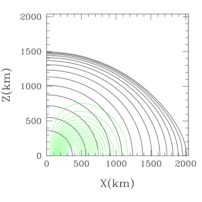
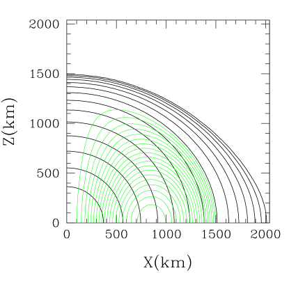
Figure 1: Initial density contour curves and magnetic field lines for model A with $n_{b}=1$ (left) and with $n_{b}=4$ (right). The density contour curves (thick, black) are drawn for $\rho=10^{10-0.5j}~{}{\rm g/cm^{3}}$ with $j=1,2,\cdots,14$, and the magnetic field lines (thin, green) are for $A_{\varphi}=A_{\varphi,{\rm max}}(1-0.05j)$ with $j=1,2,\cdots,19$ where $A_{\varphi,{\rm max}}$ denotes the maximum of $A_{\varphi}$.

V Grid setup

During the collapse, the central density increases from $10^{10}~{}{\rm g/cm^{3}}$ to $\sim 6\times 10^{14}~{}{\rm g/cm^{3}}$. This implies that the characteristic length scale of the system varies by a factor of $\sim 100$. One of the computational challenges in a stellar core collapse simulation is maintaining numerical accuracy despite the significant change in the characteristic length scale. In the early phase of the collapse (infall phase; see Sec. IV A), which proceeds in a nearly homologous manner, we may follow the collapse with a relatively small number of grid points, and successively move the outer boundary inward (while keeping the same number of grid points) to increase resolution. As the collapse proceeds, the central region shrinks more rapidly than the outer region, and hence a higher grid resolution is necessary to accurately follow such rapid collapse in the central region. On the other hand, the location of the outer boundaries cannot be changed by a large factor because this would discard matter in the outer envelope.

To follow the collapse accurately and save CPU time, we adopt the regridding technique described in SS02 ; SS04a . Regridding is carried out whenever the characteristic radius of the collapsing star decreases by a factor of 2–3. At each regridding, the grid spacing is decreased by a factor of 2. All the quantities in the new grid are calculated using cubic interpolation. To avoid discarding the matter in the outer region, we also increase the grid number at regridding, ensuring that the discarded baryon rest mass is less than 3% of the total.

Specifically, the values of $N$ and $L$ (see Sec. II.1) in the present work are chosen in the following manner. First, we define a relativistic gravitational potential $\Phi_{c}\equiv 1-\alpha_{c}~{}(\Phi_{c}>0)$, which is $\approx 0.006$ at $t=0$ for all the models chosen in this work. Since $\Phi_{c}$ is approximately proportional to $M/R$, $\Phi_{c}^{-1}$ can be used as a measure of the characteristic length scale. From $t=0$ to the time at which $\Phi_{c}=0.02$, we set $N=420$. The value of $L$ is chosen so that the equatorial radius is initially covered by 400 grid points. At $\Phi_{c}=0.02$, the characteristic stellar radius becomes approximately one third of the initial value. At this time, the first regridding is performed. The grid spacing is cut in half and the grid number is increased to $N=700$. Next, we set $N=1180$ for $0.04\leq\Phi_{c}\leq 0.08$, $N=1900$ for $0.08\leq\Phi_{c}\leq 0.16$, and $N=2500$ for $\Phi_{c}\geq 0.16$ (the minimum value of $\Phi_{c}$ is   0.25 for all the models we consider). In this treatment, the total discarded fraction of the baryon rest mass is $\sim 1\%$ for model A, $\sim 2\%$ for model B, and $\sim 2.5\%$ for model C with $(\Gamma_{1}$, $\Gamma_{2}$, $\Gamma_{\rm th}$, $\rho_{\rm nuc})=$ (1.3, 2.5, 1.3, $2\times 10^{14}~{}{\rm g/cm^{3}}$). In the following, we refer to this resolution as the standard resolution.

To check the convergence of our numerical results, we also perform simulations using higher and lower grid resolutions for model A2. In the higher-resolution case, the value of $N$ is changed as follows: $N=500$ for $\Phi_{c}\leq 0.02$, $N=840$ for $0.02\leq\Phi_{c}\leq 0.04$, $N=1420$ for $0.04\leq\Phi_{c}\leq 0.08$, $N=2268$ for $0.08\leq\Phi_{c}\leq 0.16$, and $N=2540$ for $\Phi_{c}\geq 0.16$. In this case, the equatorial radius is covered by 480 grid points initially. In the lower-resolution simulations, the equatorial radius is initially covered by 300 and 240 grid points and the values of $N$ are changed as follows: $N=320$ and 260 for $\Phi_{c}\leq 0.02$, $N=540$ and 432 for $0.02\leq\Phi_{c}\leq 0.04$, $N=900$ and 720 for $0.04\leq\Phi_{c}\leq 0.08$, $N=1440$ and 1200 for $0.08\leq\Phi_{c}\leq 0.16$, and $N=1900$ and 1520 for $\Phi_{c}\geq 0.16$. These resolutions are referred to as the high, middle, and low resolutions, respectively.

We also performed several simulations using multiple transition fisheye coordinates CLZ06 . This technique allows us to obtain high resolution in the central region with a relatively small grid number. The details of our fisheye implementation are discussed in Appendix A. We have confirmed that the results obtained using the fisheye coordinates agree with those obtained using the original coordinates.

Simulations for each model with the standard resolution are performed for about 150,000 time steps. This corresponds to the physical time of $\sim 150$ ms ($\sim 35$ ms after core bounce). At this time, most of the interesting MHD processes have occurred and the system is settling down to a stationary state. For the code of SS05 , the required CPU time for one model is about 20 CPU hours using 48 processors of FACOM VPP 5000 at the data processing center of National Astronomical Observatory of Japan, about 60 CPU hours using 8 processors of NEC SX8 at Yukawa Institute of Theoretical Physics (YITP) in Kyoto University, and about 120 CPU hours using 8 processors of NEC SX6 at ISAS, JAXA. In order to check the validity of our results, several simulations were repeated using the code of DLSS . We have confirmed that the results obtained with these two codes agree. Thus, in the following section, we mainly present the numerical results from the code of SS05 .

VI Numerical Results

VI.1 Dynamics

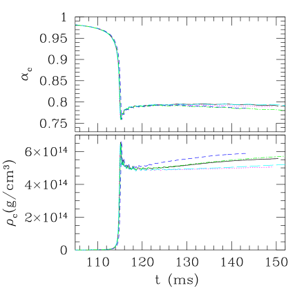
Figure 2: Evolution of the central lapse and central density for models A0 (dotted curves), A1 (long-dashed curves), A2 (solid curves), A3 (dashed curves), and A4 (dot-dashed curves).

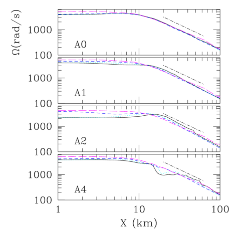
Figure 3: Evolution of the angular velocity of the resultant PNSs as a function of cylindrical radius in the equatorial plane for models A0, A1, A2, and A4. The long-dashed, dashed, dotted, and solid curves denote $\Omega$ at 118.4, 127.9, 136.7, and 149.1 ms for model A0, at 118.5, 130.6, 140.3, and 150.6 ms for model A1, and at 118.3, 131.3, 137.8, and 150.8 ms for model A2, and at 118.6, 128.0, 137.2, and 149.5 ms for model A4. The dot-dashed line segments denote the slope of $\Omega\propto\varpi^{-3/2}$.

As described in, e.g., Newton4 ; HD ; SS04a , the collapse of a rotating stellar core for which the initial $T/|W|$ is not too large (i.e., $\mathrel{\raise 1.29167pt\hbox{$<$}\mkern-14.0mu\lower 2.58334pt\hbox{$\sim$}}0.01$) and the degree of differential rotation is small ($\hat{A}\mathrel{\raise 1.29167pt\hbox{$>$}\mkern-14.0mu\lower 2.58334pt\hbox{$\sim$}}0.5$), can be divided into the following three phases. The first is the infall phase, in which the collapse sets in due to the sudden softening of the EOS. During this phase, the central density monotonically increases until it reaches nuclear density. The interior of the core that collapses nearly homologously is referred to as the inner core. The duration of the infall phase (i.e., the interval between the onset of the collapse and the time at which the central density reaches a maximum) is of order $\rho_{c}^{-1/2}$.

The second phase is the bounce, which sets in when the densities in the central region exceed nuclear density $\rho_{\rm nuc}$. At this phase, the infall of the inner core decelerates on a typical timescale of a few ms ($\sim 10\rho_{\rm nuc}^{-1/2}$). Because of its large inertia and kinetic energy, the inner core does not settle down to a stationary state immediately but overshoots and rebounds, driving outgoing shocks at the outer edge of the inner core.

The third phase is the ring-down. The bounce occurs when the central density reaches $\sim 3\rho_{\rm nuc}$ due to a sudden stiffening of the EOS (if the centrifugal force is sufficiently small at the time that the density of the inner core exceeds nuclear density). In this case, the inner core oscillates quasi-radially for about 10 ms, and then settles down to a stationary state. In the outer region, on the other hand, shock waves propagate outward, sweeping through infalling material from the outer envelope. With our simple treatment of the microphysics, the shock propagates all the way through to the surface of the outer core, which has a radius $\sim 1000$ km note1 .

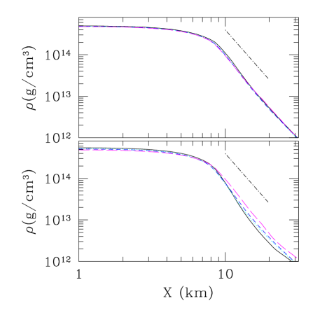
Figure 4: Evolution of the density profile of the PNSs as a function of the cylindrical radius in the equatorial plane for models A0 (upper panel) and A2 (lower panel). The profiles are given at times corresponding to those of Fig. 3. The dot-dashed line segments denote the slope of $\rho\propto\varpi^{-4}$.

Even in the presence of magnetic fields, these general features are not significantly modified as long as the field is not extremely strong (i.e., as long as the magnetic energy is smaller than the rotational kinetic energy). In Fig. 2, we show the evolution of the central lapse and central density for models A0–A4. The results for models with non-zero magnetic fields (models A1–A4) are qualitatively very similar to those for model A0, which has no magnetic field. However, the magnetic effects lead to some quantitative changes. Figure 3 shows the evolution of the angular velocity $\Omega$ for the newly-formed PNSs as a function of the cylindrical radius in the equatorial plane for models A0, A1, A2, and A4. For model A0 (see Fig. 3, upper panel), $\Omega$ relaxes to a stationary profile by $\sim 10$ ms after formation of the PNS. The remaining panels show the evolution of $\Omega$ in the presence of magnetic fields (up to $\sim 10^{16}$ G). In these cases, the PNS slows down monotonically due to outward angular momentum transport driven by magnetic braking, the MRI and the MHD outflow (see Secs. VI.2 and VI.3 for details). In particular, for model A2, in which the growth of the magnetic field by winding saturates shortly after bounce (see Fig. 6), the central spin period doubles in the first $\sim 20$ ms following the bounce. For model A1, the magnetic field is amplified more gradually (see Fig. 6). In this case, $\Omega$ does not decrease as rapidly as for model A2. For model A4, the PNS also spins down monotonically. This model has a different initial magnetic field profile from those of models A1–A3. This difference is reflected in the evolution of the angular velocity profile, which is not as smooth for A4 in the outer region of the PNS at late times. Since the magnetic field is stronger in the outer layers for model A4, the MRI is more vigorous there and the $\Omega$ profile is thus not as smooth (see also Sec. VI.2).

Figure 4 shows the evolution of the density profiles in the equatorial plane for models A0 and A2. For A0, the density profile quickly relaxes to a stationary state, while it changes with time for A2 due to the angular momentum transport. In accord with the spindown shown in Fig. 3, the central density gradually increases (see Fig. 2). Since material is ejected in an MHD-driven outflow, the density in the surface region decreases. A more detailed discussion and a qualitative explanation of the main mechanisms driving angular momentum transport and the outflow are given in Sec. VI.3.

(a)     (b)

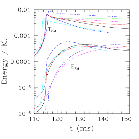
(c)

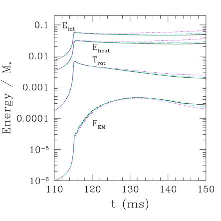
Figure 5: (a) Evolution of $E_{\rm int}$ and $E_{\rm heat}$ for models A0 (dotted curves), A1 (dashed curves), A2 (solid curves), A3 (dot-dashed curves), A4 (long-dashed curves), B (dot-long-dashed curves), and C (long-and-short dashed curves). (b) The same as (a) but for $T_{\rm rot}$, and $E_{\rm EM}$. (c) Evolution of $E_{\rm int}$, $E_{\rm heat}$, $T_{\rm rot}$, and $E_{\rm EM}$ for model A2 with different grid resolutions. The dotted, solid, dashed, and dot-dashed curves denote the results in the high-, standard-, middle-, and low-resolution runs.

In Figs. 5(a) and (b), we show the various energies ($E_{\rm int}$, $E_{\rm heat}$, $T_{\rm rot}$, and $E_{\rm EM}$) as functions of time for models A0–A4, B, and C. All of the energies increase during the infall phase and reach their maxima at the bounce. Following the bounce, $E_{\rm int}$ and $E_{\rm heat}$ relax to values of a quasistationary state which change very slowly (see Fig. 5(a)). On the other hand, $T_{\rm rot}$ rapidly decreases in the presence of the magnetic field, reflecting the spindown of PNSs by magnetic effects (see Fig. 5(b)). The rate of this decrease is larger for larger values of $E_{\rm EM}$, as anticipated in Sec. III.5.

Figure 5(c) shows the evolution of $E_{\rm int}$, $E_{\rm heat}$, $T_{\rm rot}$, and $E_{\rm EM}$ for model A2 with different grid resolutions. With the middle and low resolutions, convergence is not well achieved. On the other hand, the results in the high and standard resolutions agree well, indicating that the standard resolution is an appropriate choice for this problem.

The simulations for models B and C are performed with the same initial magnetic field profile and field strengths as models A2 and A1, respectively (see Table II), and the results for the various energies are shown together in Fig. 5. It is found that the evolutions for models B and C proceed in the same qualitative manner as for models A2 and A1, respectively. Quantitatively, the initial rotational kinetic energy is reflected in the evolution of $T_{\rm rot}$ and $E_{\rm EM}$. For model B, the maximum rotational kinetic energy is smaller than that for model A2. As a result, the growth rate of the magnetic energy after bounce due to winding as well as the resulting maximum value reached are smaller. Thus, the magnetic energy achieved at saturation for a particular model depends on the rotational kinetic energy. This is expected since the magnetic energy is ultimately drawn from the energy stored in differential rotation. For model C, $T_{\rm rot}$ at bounce is larger than that of model A1 because of the differential rotation at the onset of collapse and resulting larger rotation velocity of the PNS. As a result, the growth rate of $E_{\rm EM}$ and the maximum value reached are larger than those for model A1.

VI.2 Evolution of the magnetic field

Figure 3 shows that for $\varpi\mathrel{\raise 1.29167pt\hbox{$<$}\mkern-14.0mu\lower 2.58334pt\hbox{$\sim$}}10$ km (i.e., in the central region of the PNSs), the angular velocity has a roughly flat profile. With so little differential rotation, the magnetic field does not grow much, either by winding or the MRI. MHD effects have little influence on the evolution in this region. For $\varpi\mathrel{\raise 1.29167pt\hbox{$>$}\mkern-14.0mu\lower 2.58334pt\hbox{$\sim$}}10$ km (i.e., near the surface and outside the PNSs), the angular velocity is approximately Keplerian (i.e., $\Omega\propto\varpi^{-3/2}$; see the dot-dashed line segments in Fig. 3). Because of the strong differential rotation, the outer region with $\varpi\mathrel{\raise 1.29167pt\hbox{$>$}\mkern-14.0mu\lower 2.58334pt\hbox{$\sim$}}10$ km is subject to winding and the MRI (see Secs. III.2 and III.3). In particular, the magnetic field is rapidly amplified in the region with $\varpi\approx 10$–30 km, where both the angular velocity and the degree of differential rotation are large. We note that strong differential rotation results even for rigidly rotating progenitors.

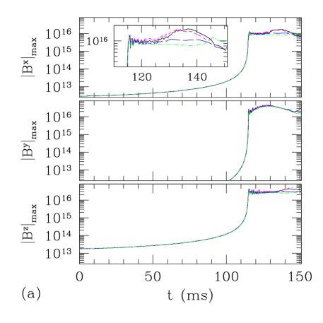
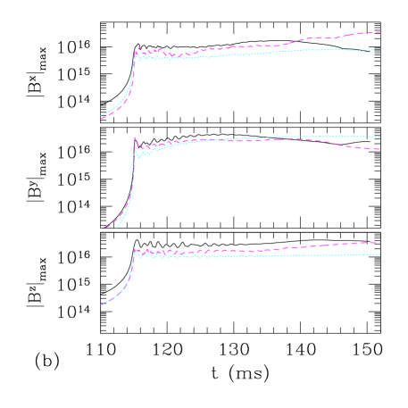
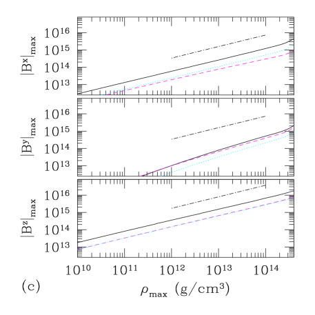
Figure 6: (a) Evolution of $|B^{i}|$ for model A2. The solid, dashed, long-dashed, and dot-dashed curves denote the results from the standard, high, middle, and low resolution runs for model A2. The enlarged panel for the evolution of $|B^{x}|_{\rm max}$ illustrates that the growth of the field strength by the MRI is well resolved only in the high and standard runs. (b) The same as (a) but for models A1 (dotted curves), A2 (solid curves), and A4 (dashed curves) with the standard resolution. (c) $|B^{x}|_{\rm max}$ as a function of $\rho_{\rm max}$ during infall phase for models A1 (dotted curves), A2 (solid curves), and A4 (dashed curves) with the standard resolution. The dot-dashed line segments above the three curves denote the relation $|B^{i}|_{\rm max}\propto\rho_{\rm max}^{2/3}$.

In Fig. 6, we show the evolution of the maximum values of $|B^{i}|$ for models A1, A2, and A4. Note that, in our setup, $B^{x}$ and $B^{z}$ are the poloidal field components ($B^{x}=B^{\varpi}$) and $B^{y}$ is the toroidal component ($B^{y}=\varpi B^{\varphi}=B^{T}$) since we assume axisymmetry and solve the equations in $x$-$z$ plane. To demonstrate the effects of the grid resolution, the results for four different resolutions are displayed together for model A2.

During the infall phase, the magnetic field is amplified monotonically: The poloidal field grows due to the compression of matter, while the toroidal field grows primarily by winding (cf. Sec. III.1). In the ideal MHD approximation, the magnetic field lines are frozen into the plasma, and hence, the poloidal field strength should grow approximately as $\rho^{2/3}$ (see Sec. III.1). As shown in Fig. 6(c), this relationship holds for the maximum poloidal field components over several decades of growth in the density. Since $B^{y}$ grows by winding, its growth accelerates rapidly just before the bounce due to the rapid growth of $|B^{x}|$. As shown in Fig. 6, a significant amplification indeed occurs for about 2–3 ms before the bounce at $t\approx 115$ ms. Figure 6(c) also shows that the maximum value of the toroidal magnetic field increases slightly faster than $\rho^{2/3}$ during the infall phase. This qualitatively agrees with the estimate in Sec. III.1.

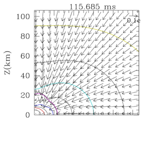
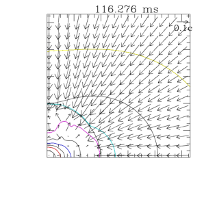
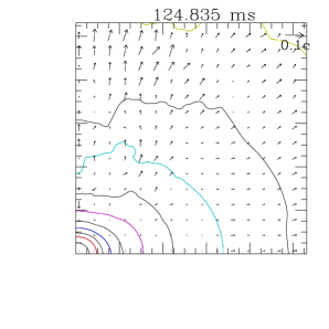
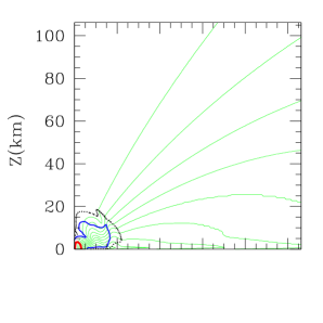
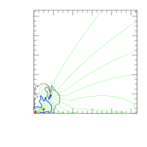
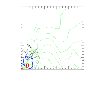
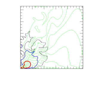
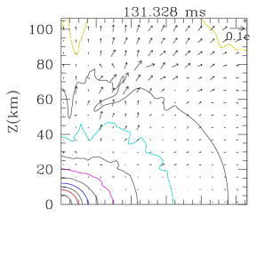
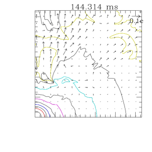
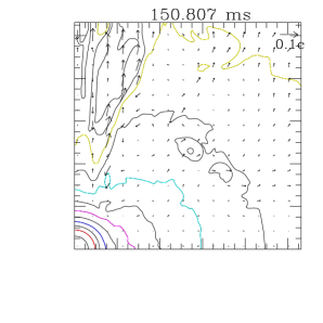
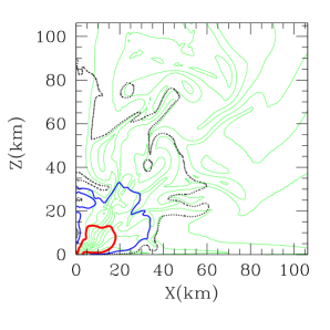
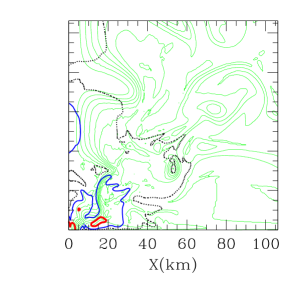
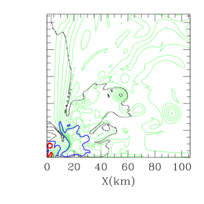
Figure 7: Density contour curves and velocity vectors for model A2 (first and third rows). The contours are drawn for $\rho=10^{15-0.5i}~{}{\rm g/cm^{3}}~{}(i=1$–12). (The red, blue, magenta, cyan, and yellow curves denote $\rho=10^{14}$, $10^{13}$, $10^{12}$, $10^{11}$, and $10^{10}~{}{\rm g/cm^{3}}$, respectively.) The scale of the velocity is shown in the upper-right corner. The second and fourth rows show the poloidal magnetic field lines (green) and contours of the magnetic pressure (thick red, blue, and normal black curves) at corresponding times. The poloidal magnetic field lines are drawn as contours of $A_{\varphi}$, with levels given by $A_{\varphi}=(1-0.1i)A_{\varphi,{\rm max}}~{}(i=0$–9). Here, $A_{\varphi,{\rm max}}$ is the maximum value of $A_{\varphi}$ at each time slice. The contour curves of the magnetic pressure are drawn for $10^{30}$ (very thick red curves), $10^{29}$ (thick blue curves), and $10^{28}~{}{\rm dyn/cm^{2}}$ (thick black dotted curves).

To provide an overview of the evolution, we display snapshots of density contours, velocity vectors, poloidal magnetic field lines, and magnetic pressure contours for model A2 at selected time slices in Fig. 7. In Fig. 8, the evolution of the magnetic field strength as a function of the cylindrical radius is shown for selected coordinate values of $z$. (We do not plot $B^{x}$ and $B^{y}$ on the equatorial plane since they vanish there by symmetry.) We find that, after the bounce at $t\approx 115$ ms, shock waves propagate outward. Material behind the shocks moves outward in an anisotropic manner due to the rotation and to the anisotropic density profile of the collapsing star. This matter outflow is strongest along the rotation axis.

For $t\mathrel{\raise 1.29167pt\hbox{$>$}\mkern-14.0mu\lower 2.58334pt\hbox{$\sim$}}120$ ms, differential rotation modifies the profile of the magnetic field and amplifies the magnetic pressure (see Figs. 6, 7, and Fig. 8). As Fig. 6 shows, the toroidal field continues to grow after bounce because of the differential rotation near the surface and outside of the PNS. The magnetic pressure monotonically increases for 120 ms $\mathrel{\raise 1.29167pt\hbox{$<$}\mkern-14.0mu\lower 2.58334pt\hbox{$\sim$}}t\mathrel{\raise 1.29167pt\hbox{$<$}\mkern-14.0mu\lower 2.58334pt\hbox{$\sim$}}130$ ms in the region $\varpi=10$–30 km and $z\mathrel{\raise 1.29167pt\hbox{$<$}\mkern-14.0mu\lower 2.58334pt\hbox{$\sim$}}10$ km. This is reflected in the third through fifth snapshots in Fig. 7, which show that the region with $P_{\rm mag}\geq 10^{30}~{}{\rm dyn/cm^{2}}$ expands. We note that the amplification at $z=0$ is very small since we impose the symmetry condition that $B^{x}$ and $B^{y}$ must vanish on the equatorial plane. Comparison of Figs. 5 and 6 illustrates that the increase of the magnetic energy is primarily due to the growth of the toroidal field. This growth stops when the magnetic energy reaches about 10–20% of the rotational kinetic energy irrespective of the initial field strength and profile (cf. Fig. 5). Figure 6 shows that the toroidal field growth can be followed well even for the lower grid resolutions.

The growth of magnetic energy saturates when back-reaction from magnetic braking becomes significant. This occurs at a time comparable to the Alfvén crossing time Shapiro $t_{\rm sat}\approx t_{\rm A}$, where $t_{A}$ is given by Eq. (58). For the models considered here, $t_{\rm A}\mathrel{\raise 1.29167pt\hbox{$<$}\mkern-14.0mu\lower 2.58334pt\hbox{$\sim$}}30$ ms. From the numerical results for model A2, we see that $t_{\rm sat}\sim 10$ ms (see Fig. 6).

The toroidal magnetic field would not achieve the saturation strength described above if significant magnetic reconnection were to operate before magnetic braking could take effect. However, the velocity of fluid entering the dissipation layer is expected to be a small fraction (probably $10^{-1}$ or $10^{-2}$) of the Alfvén velocity (see, e.g. parker ; priest ; Kulsrud ). Simple estimates show that this expectation is borne out in the solar magnetosphere and the geomagnetic tail of the earth Kulsrud . Thus, the reconnection timescale should, in general, be of order 10 to 100 times longer than the Alfvén timescale which governs the growth of the toroidal field. On the timescales of interest for PNS evolution considered here, reconnection will thus not play an important role.

Following saturation, the toroidal field strength begins to decrease in the central region due to magnetic braking. This is reflected in the decrease of the magnetic pressure for $\varpi\sim 10$ km and $z\sim 10$ km seen in the sixth and seventh snapshots of Fig. 7. Magnetic braking also leads to outward transport of angular momentum by Alfvén waves. This is clearly seen in the middle panel of Fig. 8; $|B^{y}|$ decreases for $\varpi\mathrel{\raise 1.29167pt\hbox{$<$}\mkern-14.0mu\lower 2.58334pt\hbox{$\sim$}}15$ km but increases for $\varpi\mathrel{\raise 1.29167pt\hbox{$>$}\mkern-14.0mu\lower 2.58334pt\hbox{$\sim$}}15$ km. The middle and lower panels of Fig. 3 also show that the angular velocity in the central region decreases while it increases for $10~{}{\rm km}\mathrel{\raise 1.29167pt\hbox{$<$}\mkern-14.0mu\lower 2.58334pt\hbox{$\sim$}}\varpi\mathrel{\raise 1.29167pt\hbox{$<$}\mkern-14.0mu\lower 2.58334pt\hbox{$\sim$}}50$ km for models A1 and A2. This angular momentum transport drives matter outflow at relatively low latitude (see for $t\mathrel{\raise 1.29167pt\hbox{$>$}\mkern-14.0mu\lower 2.58334pt\hbox{$\sim$}}130$ ms in Fig. 7). However this outflow is not as strong as that along the rotation axis note2 .

At bounce, the compression stops and so does the rapid global growth of the poloidal field. However, the poloidal field in the outer region of the PNSs (see Fig. 7) continues to grow after the bounce by the MRI. Figure 7 indicates that the poloidal field lines for $\varpi\approx 10$–30 km and $z=10$–50 km are highly distorted for $t\mathrel{\raise 1.29167pt\hbox{$>$}\mkern-14.0mu\lower 2.58334pt\hbox{$\sim$}}130$ ms. Evidence of the MRI is also seen in the first and third panels of Fig. 8 which show that initially smooth poloidal fields become highly inhomogeneous and the amplification is locally enhanced note2 (the local amplification can be seen clearly in the region $R\sim 35$ km in the $B^{x}$ plot in Fig. 8).

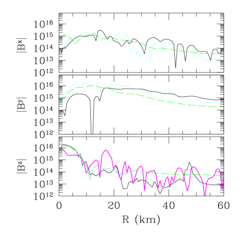
Figure 8: Evolution of $|B^{x}|$ and $|B^{y}|$ at $z\approx 14.2$ km and $|B^{z}|$ in the equatorial plane as a function of the cylindrical radius for model A2. The solid, dotted, and dashed curves denote the data for $t=150.8$, 137.8, and 118.3 ms. The thick solid curve for $|B^{z}|$ is the result at $z\approx 10$ km at $t=150.8$ ms.

The growth $|B^{x}|_{\rm max}$ shown in Fig. 6(a) demonstrates the importance of resolution in capturing the MRI. In this figure, we plot results for four different resolutions. In the low and middle resolutions, the maximum value of $|B^{x}|$ increases until the bounce and holds steady thereafter. On the other hand, there is significant growth after the bounce in the standard and high resolution runs. Note that the wavelength of the fastest-growing mode of the MRI, $\lambda_{\rm max}$, is a few km for $B\sim 10^{14}$ G, $\rho\sim 10^{13}~{}{\rm g/cm^{3}}$, and $\Omega\sim 10^{3}~{}{\rm rad~{}s}^{-1}$ [cf. Eq. (66)] which are typical values in the outer region of the PNS. In the standard resolution, the grid spacing is $\sim 0.1\lambda_{\rm max}$, and the MRI is marginally resolved, but it is unresolved for the low and medium resolutions. This illustrates that, in MHD simulations, integrations with several grid resolutions are essential for correctly identifying the physical mechanisms at work.

Figures 6(a) and (b) show that $|B^{z}|_{\rm max}$ does not increase significantly. This does not imply that $|B^{z}|$ does not change due to the MRI. Indeed, we find that the $z$-component is amplified in the outer regions of the PNSs (see Fig. 8). However, these local fluctuations are not as large as $B^{z}$ in the central part of the PNSs (where the $z$-component dominates and is fairly constant following the PNS formation).

The amplification of the magnetic field by the MRI is seen at $\sim\!10$ ms after the bounce. The estimated growth time scale of the MRI is $t_{\rm MRI}\approx 4/3\Omega$ [cf. Eq. (65)] which is a few milliseconds for $\varpi=10$–30 km. Our simulation indicates that the actual $t_{\rm MRI}$ is somewhat longer than this estimate. The tendency for the linear analysis to underestimate the MRI growth time is also seen in our previous results for the evolution of magnetized neutron stars DLSSS2 . The linear analysis may be inaccurate by a factor of several in the present context since the MRI is treated as a purely local phenomenon, assuming a uniform background state over length scales much longer than the wavelengths of the perturbations. However, since the expected value of $\lambda_{\rm max}$ is only one order of magnitude smaller than the characteristic radius, this assumption may not hold. To understand the growth timescale of the MRI in the PNS, a global analysis is necessary. Indeed, a global stability analysis for magnetized accretion disks shows that the local analysis overestimates the growth rate CPS .

As in the case of the toroidal field, the growth of the poloidal field saturates when $|B^{x}|_{\rm max}$ reaches $\sim\!2$–$3\times 10^{16}$ G. The saturation may be partly due to the limited grid resolution (i.e., due to numerical diffusion), but this effect does not seem to be very large since the value of $|B^{x}|_{\rm max}$ is approximately the same for the high and standard resolutions (see Fig. 6).

The contribution to the growth of the magnetic field strength by winding is significantly larger than the contribution from the MRI. Indeed, we find that the average value of the poloidal field is smaller than that of the toroidal field. Because MRI is a local instability, it does not increase the global magnetic energy as significantly as winding.

After the saturation of the field growth by winding and the MRI, a collimated and nearly stationary magnetic field with $|B^{z}|\gg|B^{\varpi}|$ is formed near the rotation axis (see the last snapshot of Fig. 7). For the high latitude regions with $z\mathrel{\raise 1.29167pt\hbox{$>$}\mkern-14.0mu\lower 2.58334pt\hbox{$\sim$}}50$ km and with $\varpi\mathrel{\raise 1.29167pt\hbox{$>$}\mkern-14.0mu\lower 2.58334pt\hbox{$\sim$}}10$ km, the absolute value of the toroidal component $|B^{y}|$ is as large as $|B^{z}|$, indicating a helical magnetic field. (On the other hand, very near the rotation axis, $|B^{z}|$ is much larger than $|B^{y}|$). The field strength at $t\sim 150$ ms is $\mathrel{\raise 1.29167pt\hbox{$>$}\mkern-14.0mu\lower 2.58334pt\hbox{$\sim$}}10^{15}$ G at $z=100$ km. Since the degree of differential rotation is small near the rotation axis, this magnetic field configuration is stable. A nearly stationary outflow is driven along the collimated field lines. This is probably due to the magneto-centrifugal mechanism (cf. Sec. III.5), and we discuss this possibility in more detail in Sec. VI.3. In contrast to the region near the axis, the toroidal field is much stronger than the poloidal field at large cylindrical radius.

We find that the evolution path of the magnetic field depends quantitatively (but not qualitatively) on the initial field strength and profile. In the right panel of Fig. 6, we show the evolution of each component of the magnetic field for models A1, A2, and A4 (see also Fig. 5). For A1, the initial magnetic field profile is the same as that for A2 while the initial strength is weaker. The evolution of the magnetic field is similar for these two models except that, for A1, it takes longer to amplify the magnetic field because of the smaller initial value of $B^{\varpi}$.

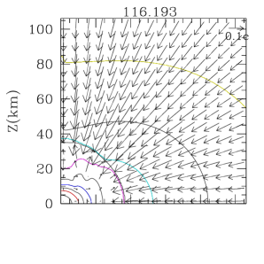
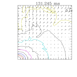
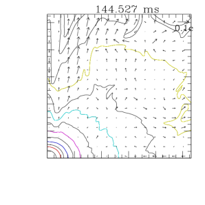
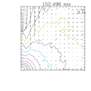
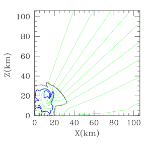
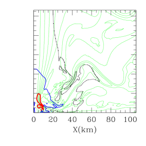
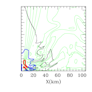
Figure 9: Evolution of the density contour curves and velocity vectors for model A4. The contours and velocity vectors are drawn in the same manner as in Fig. 7.

Model A4 has a different initial magnetic field profile from that of models A1 and A2. Since the magnetic field is initially distributed over a larger range of cylindrical radii for A4 (see Fig. 1), field growth by compression is more efficient for A4. Although the maximum values of the magnetic field are initially identical for models A1 and A4 (see Table II), those at bounce are larger for model A4. Model A4 also has a different field configuration after bounce than A1 and A2. In Fig. 9, we show snapshots of the density contours, the velocity vectors, the magnetic field lines, and contour curves of the magnetic pressure after the formation of the PNS for model A4. By comparison between Fig. 7 and Fig. 9 at $t\approx 116$ ms, it is found that the fraction of the $z$-component of the magnetic field is larger for model A4 than for model A2. This strong vertical field is advantageous for inducing the MRI. In addition, a stationary collimated field is formed more quickly for A4 than for A2. This results in a stronger MHD outflow (see Sec. VI.3).

VI.3 MHD outflow

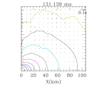
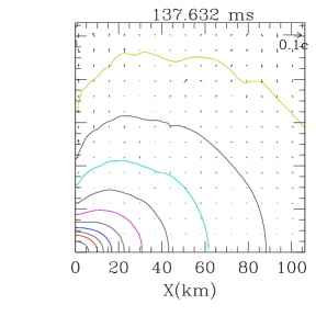
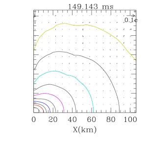
Figure 10: Evolution of the density contours and velocity vectors for model A0. The contours and velocity vectors are drawn in the same manner as in Fig. 7.

Both winding and the MRI increase the magnetic stress in the outer regions of PNSs which have large degrees of differential rotation. This stress induces an MHD outflow, particularly near the rotation axis (see velocity vectors of Figs. 7 and 9 for $t\mathrel{\raise 1.29167pt\hbox{$>$}\mkern-14.0mu\lower 2.58334pt\hbox{$\sim$}}130$ ms). To prove that this is indeed due to the magnetic stress, in Fig. 10, we show evolution of the density contour curves and velocity vectors for model A0, which has no magnetic field. In this model, the PNS relaxes to a stationary state for $t\mathrel{\raise 1.29167pt\hbox{$>$}\mkern-14.0mu\lower 2.58334pt\hbox{$\sim$}}130$ ms. Comparing Figs. 7, 9, and 10, it is evident that the MHD outflow is driven by magnetic effects. One also sees that the density profile changes due to the matter outflow (especially near the rotation axis) and that the oblateness of the PNSs for models A2 and A4 is smaller than for model A0 at $t\approx 150$ ms due to the angular momentum loss (compare the density contour curves of $\rho=10^{12}~{}{\rm g/cm^{3}}$ for the three models in the final snapshots).

We posit three possible sources for the MHD outflow: the magneto-spring mechanism, turbulence induced by the MRI, and the magneto-centrifugal mechanism. In the early phase, winding amplifies the toroidal field and the magneto-spring mechanism works efficiently to drive the MHD outflow. This outflow blows off matter preferentially in the $z$-direction. However, it is not sharply collimated; the half-opening angle is $\sim 45$ degrees. Turbulent motion caused by the MRI also induces an outflow. In contrast to the magneto-spring mechanism, however, the MRI-driven outflow is incoherent.

After the toroidal magnetic field saturates, a stationary, collimated, helical magnetic field forms around the rotation axis. Matter then flows out along the collimated field lines for $t\mathrel{\raise 1.29167pt\hbox{$>$}\mkern-14.0mu\lower 2.58334pt\hbox{$\sim$}}150$ ms in case A2 and for $t\mathrel{\raise 1.29167pt\hbox{$>$}\mkern-14.0mu\lower 2.58334pt\hbox{$\sim$}}140$ ms in case A4, as shown in Figs. 7 and 9. This suggests that the magneto-centrifugal mechanism (see Sec. III.5) is operating. This interpretation can be inferred indirectly from two facts: (i) the MHD outflow is continuously ejected from the PNS, even after the growth of the toroidal field by winding saturates, and (ii) the outflow is absent in the region very close to the rotation axis. This indicates that the outflow is driven along the collimated magnetic field with an appropriate inclination angle between the rotation axis and the poloidal field lines, as is necessary for magneto-centrifugal launching BP ; BP1 .

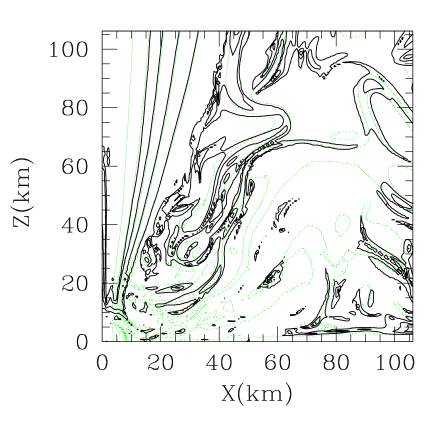
Figure 11: Contour of $k=\rho_{*}v^{P}/{\cal{B}}^{P}$ (solid curves) and magnetic field lines (dotted curves) at $t=152.5$ ms for model A4. The magnetic field lines are drawn in the same manner as in Fig. 7. The contours of $k$ are drawn for $k=6\times 10^{4-0.4i}~{}{\rm g/(cm^{2}~{}s~{}G)}~{}(i=0$–4). We note that these contours are drawn only for the values of $k$ found for material on the collimated field lines.

Further evidence is found by confirming that the quantities $k\equiv\rho_{*}v^{P}/{\cal{B}}^{P}$, which should be constant along the field lines in a stationary state are actually constant (see Mestel ; BP and Appendix B). Here $v^{P}$ and ${\cal{B}}^{P}$ denote the poloidal components of $v^{i}$ and ${\cal{B}}^{i}$. Note that the definition of $k$ accounts for general relativistic corrections through $\rho_{*}$ and ${\cal{B}}^{P}$. In Fig. 11, we show the contour curves for $k$ together with the magnetic field lines at $t=152.5$ ms for model A4. It is found that the two sets of curves overlap in the region of the collimated magnetic field lines, verifying that the structure of the magnetic field is almost stationary in this region. On the other hand, the two sets of curves do not overlap for the turbulent region far from the rotation axis.

To give a better overall picture of the outflow, we show in Fig. 12 the density contours, velocity vectors, and poloidal magnetic field lines at $t=152.5$ ms for model A4. In this figure, a larger region than that shown in the last panel of Fig. 9 is displayed. For $r\mathrel{\raise 1.29167pt\hbox{$>$}\mkern-14.0mu\lower 2.58334pt\hbox{$\sim$}}200$ km, a weakly-anisotropic outflow is found. However, the velocity of the matter near the rotation axis is relatively large. For $r\mathrel{\raise 1.29167pt\hbox{$<$}\mkern-14.0mu\lower 2.58334pt\hbox{$\sim$}}200$ km, on the other hand, the strong outflow is seen only along the collimated magnetic field in the vicinity of rotation axis. The greatly enhanced strength of the outflow along the collimated field lines points to magneto-centrifugal launching as a likely driver of the outflow. Our results suggest that jets may be launched during supernova explosions if the collimated magnetic fields found here are generic WMW ; AHM ; MBA . For $r\mathrel{\raise 1.29167pt\hbox{$<$}\mkern-14.0mu\lower 2.58334pt\hbox{$\sim$}}200$ km, a slower, incoherent flow pattern is also seen, reflecting the continuous driving of irregular matter motions by the MRI.

As mentioned in Sec. III.5, the magneto-centrifugal launching mechanism requires a mechanism for ejecting material outward at the base. This is particularly important if the opening angle of the collimated field line is small BP ; BP1 . In the present case, the magnetic field is significantly perturbed in the vicinity of the PNSs by the MRI. Turbulence and/or irregular Poynting flux generated by the MRI could serve to inject material into the magneto-centrifugal wind.

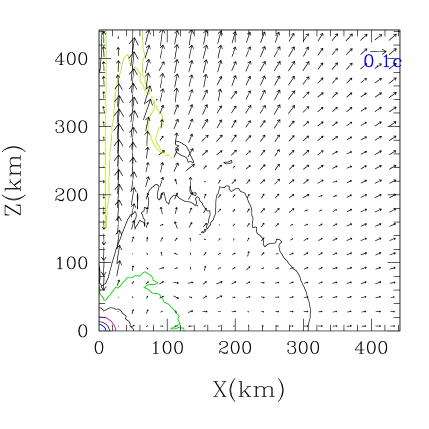
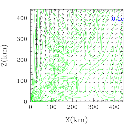
Figure 12: The density contours and velocity vectors (left) and the poloidal magnetic field lines and velocity vectors (right) at $t=152.5$ ms for model A4. The density contours are drawn for $\rho=10^{15-i}~{}{\rm g/cm^{3}}~{}(i=1$–7). The velocity vectors and poloidal magnetic field lines are drawn as in Fig. 7.

In addition to rest mass, energy and angular momentum are also carried away from the PNS by the outflows. In Fig. 13 we show $F_{M}$, $F_{e}$, and $F_{J}$ evaluated at $r=L/4$ ($\approx 224$ km for models A0–A4, $\approx 143$ km for model B, and $\approx 161$ km for model C) as a function of time for models A0–A4, B, and C. We also evaluated the fluxes at other radii and found that, aside from a time shift, the results depend weakly on the radius.

In the early ringdown phase in which shocks propagate outward, the loss of mass, energy, and angular momentum from the system is due primarily to the matter outflow (as opposed to the Poynting outflow) irrespective of the presence of magnetic field. Hence $F_{M}$, $F_{e}$, and $F_{J}$ are roughly independent of the field strength (compare results for model A0, A1, A2, and A4). In the absence of the magnetic field (model A0; dot-dashed curves), however, the outflow rates decay in an exponential manner, leaving a stationary PNS. On the other hand, in the presence of the magnetic field, the fluxes remain nonzero, and the PNSs continuously lose mass, energy, and angular momentum. The evolution of the fluxes for model A1 show that the dominance of the MHD-driven outflow over the shock-driven outflow is delayed for $\sim 10$ ms after bounce, i.e. after the toroidal field becomes sufficiently strong. (Note that for model A1, the growth of the toroidal field by winding saturates at the relatively late time of $\sim 30$ ms after bounce. This is consistent with the fact that the MHD-driven outflow becomes dominant later for this model than for A2–A4.)

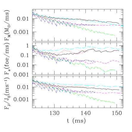
Figure 13: $F_{M}$, $F_{e}$, and $F_{J}$ at $r\approx 224$ km for models A0 (dot-long-dashed curves), A1 (dashed curves), A2 (solid curves), A4 (long-dashed curves), B (dotted curves), and C (dot-dashed curves). The abbreviation ’foe’ denotes $10^{51}$ ergs, while $J_{0}$ is the initial value of $J$.

The strength of the outflow depends on the initial magnetic field strength (compare the results of models A1 and A2). This is due to the difference in the resulting ratio of the poloidal field strength to the toroidal field strength $C_{B}$ for the PNS [see Eq. (70)]. The toroidal fields are wound up to similar saturation strengths in the various models regardless of the initial poloidal field strength (see Fig. 6). On the other hand, after bounce, the poloidal field is not uniformly amplified, though the MRI increases the strength locally. As a result, the value of $C_{B}$ is smaller for model A1 and consequently so are the values of $F_{M}$, $F_{e}$, and $F_{J}$.

In addition to the magnitude of the initial seed magnetic field, the strength of the outflow (and particularly of the magneto-centrifugal outflow), also depends strongly on the initial field profile. The relative size of the $z$-component of the magnetic field is larger for model A4 than for model A2 (compare Figs. 7 and 9). The larger $z$-component is favorable for inducing the MRI and the resulting MHD outflow, although the magnetic energy of the PNSs for models A2 and A4 are nearly identical (see Fig. 5).

Although the outflow rates depend on the initial magnetic field profile and strength, the ratio of $F_{J}/F_{M}\sim 1.5$–$2.5J/M$ is always larger than $J/M$ for all cases considered here. Thus, the MHD outflow carries away material with a larger specific angular momentum than that of the PNSs, leading to spindown. Figure 13 shows that the spindown time scale $J_{0}/F_{J}$ ($J_{0}$ is the initial value of $J$) is $\sim$100–300 ms for models A1, A2, and A4, and is approximately proportional to $C_{B}^{-1}$ [see Eq. (70) and note that the value of $C_{B}$ for A2 is about twice of that for A1]. Since $C_{B}\mathrel{\raise 1.29167pt\hbox{$>$}\mkern-14.0mu\lower 2.58334pt\hbox{$\sim$}}0.1$ is indicated by our simulations, a large amount of the angular momentum of the PNSs is carried away within $\sim 1$ s after the onset of the MHD outflow.

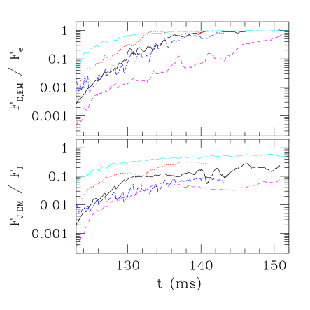
Figure 14: $F_{E,{\rm EM}}/F_{e}$ and $F_{J,{\rm EM}}/F_{J}$ for models A1 (dashed curves), A2 (solid curves), A4 (long-dashed curves), B (dotted curves), and C (dot-dashed curves).

In Fig. 14, we show the ratios of $F_{E,{\rm EM}}/F_{e}$ and $F_{J,{\rm EM}}/F_{J}$ as functions of time for models A1, A2, A4, B, and C. The plot indicates that the outflow is largely Poynting dominated. The ratio of the EM flux to the total flux clearly depends on the initial magnetic field strength and profile. Comparing the results shown in Fig. 14, $F_{E,{\rm EM}}/F_{e}$ and $F_{J,{\rm EM}}/F_{J}$ are larger for larger values of $F_{M}$ and $F_{J}$ note3 .

The large relative fraction of the Poynting flux at radii around $\sim 200$ km also implies that, during the outward propagation of the magnetic energy, conversion to matter kinetic energy is suppressed in our model. In realistic supernovae, shock waves formed at bounce do not propagate outward unimpeded but rather stall at a radius $\sim 150$–200 km, forming a standing shock Wilson ; Janka ; Lieb ; Burrow . Thus, the MHD outflow driven from the PNS will eventually hit the stalled shock, where the Poynting energy flux as well as the kinetic energy of the matter outflow may be converted to thermal energy. The total energy from the outflow during the 10 ms period following the relaxation of $F_{M}$ to a roughly constant value is $\mathrel{\raise 1.29167pt\hbox{$>$}\mkern-14.0mu\lower 2.58334pt\hbox{$\sim$}}10^{50}$ ergs for all of the models. If this energy were converted to thermal energy at the stalled shock, it could play a significant role in driving the supernova explosion, as pointed out in TQB ; ABM ; MBA .

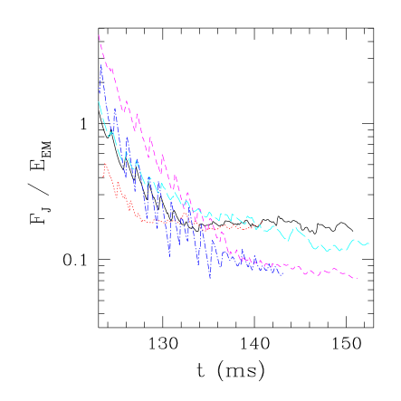
Figure 15: $F_{J}/E_{\rm EM}$ for models A1 (dashed curve), A2 (solid curve), A4 (long-dashed curve), B (dotted curve), C (dot-dashed curve).

In Fig. 15, the ratio of $F_{J}$ to $E_{\rm EM}$ is shown for models A1, A2, A4, B, and C. By Eq. (72), this ratio should be of order $C_{B}$ if the MHD outflow theory BP holds in the vicinity of the PNS. Figure 15 shows that, in the early phase ($t\mathrel{\raise 1.29167pt\hbox{$<$}\mkern-14.0mu\lower 2.58334pt\hbox{$\sim$}}130$ ms) in which matter outflow driven by shocks is dominant, the value $F_{J}/E_{\rm EM}$ decreases steeply. However, once the MHD outflow dominates, the ratio relaxes to an approximately constant value of $\sim 0.1$–0.2 for all of the models. (Our simulations indicate that $C_{B}=|B^{P}|/|B^{T}|\sim 0.1$–1 for these models.) We also find that its value for model A1 is about half as large as the values for models A2 and A4, reflecting the smaller value of $C_{B}$ for model A1. Thus, our results agree qualitatively with the MHD outflow theory. The MHD outflows found here are ultimately powered by rotation. Thus, the outflow is expected to weaken as the PNSs spin down, although at least in the first few tens of milliseconds after the saturation of the field growth, the strength is approximately constant as shown in Fig. 15.

VI.4 Outflow-induced spindown of the PNSs

Assuming that the PNSs spin down due to the MHD outflow, the loss rate of the angular momentum is described by Eq. (72) with $\eta_{*}=O(1)$. The spin angular momentum of the PNS is approximately written by $J_{*}=I_{*}\Omega_{*}$ where $I_{*}$ is a moment of inertia and $\Omega_{*}$ is an average angular velocity. After the saturation of the magnetic field growth, $E_{\rm EM}$ is approximately equal to $\zeta T_{\rm rot}$, where $\zeta$ is around 0.1–0.2 according to our results (see Fig. 5), and where $T_{\rm rot}$ is approximately $I_{*}\Omega_{*}^{2}/2$. Gathering these results, we have a relation for the evolution of the angular momentum of the PNS:

$${d(I_{*}\Omega_{*})\over dt}\approx-{\zeta\eta_{*}\over 2}I_{*}\Omega_{*}^{2}C_{B}.$$ (80)

Assuming that $I_{*}$ and $C_{B}$ are constant, we then have

$${dP_{*}\over dt}={d\over dt}\biggl{(}{2\pi\over\Omega_{*}}\biggr{)}\approx\pi\zeta\eta_{*}C_{B},$$ (81)

where $P_{*}=2\pi/\Omega_{*}$. Equation (81) suggests that the rotational period increases linearly with time as

$$P_{*} \approx P_{0}+\pi\zeta\eta_{*}C_{B}t$$ (82)

$$\approx P_{0}+30\biggl{(}{\zeta\over 0.1}\biggr{)}\biggl{(}{\eta_{*}\over 0.1}\biggr{)}\biggl{(}{C_{B}\over 0.1}\biggr{)}\biggl{(}{t\over 10~{}{\rm s}}\biggr{)}~{}{\rm ms},$$

where $P_{0}$ is the initial value of $P_{*}$. The value of $C_{B}$ during the stationary MHD outflow phase is somewhat unclear for a real system. Our present result, however, indicates that $|B^{P}|\sim|B^{T}|$ near the rotation axis, giving $C_{B}\sim 0.1$–1.

Figure 16: $P_{*}$ as a function of time for model A4.

In Fig. 16, we show the evolution of $P_{*}$ for model A4, in which the PNS and magnetic field lines reach a quasistationary state for $t\mathrel{\raise 1.29167pt\hbox{$>$}\mkern-14.0mu\lower 2.58334pt\hbox{$\sim$}}140$ ms. To obtain $P_{*}$, we compute $\Omega_{*}$ from

$$\Omega_{*}=\Big{[}\int_{\rho\geq 10^{-3}\rho_{\rm nuc}}\rho_{*}\Omega d^{3}x\Big{]}\Big{/}\Big{[}\int_{\rho\geq 10^{-3}\rho_{\rm nuc}}\rho_{*}d^{3}x\Big{]}.$$ (83)

The figure shows that the average spin period increases approximately linearly in time for $t\mathrel{\raise 1.29167pt\hbox{$>$}\mkern-14.0mu\lower 2.58334pt\hbox{$\sim$}}140$ ms. This agrees with Eq. (82). For this case, we find $dP_{*}/dt\approx 0.013$. Thus the order of magnitude for the spindown rate is in agreement with Eq. (81).

The rapid spindown will continue until the rotation in the vicinity of the PNS becomes sufficiently uniform, i.e., until the magnetic field relaxes approximately to a stationary state. If the magnetic field is amplified until saturation with $\zeta\sim 0.1$ shortly after bounce, and if the degree of differential rotation remains high for $\sim 1000$ s after the saturation, the rotation will slow to a period longer than $\sim 1$ s. For poloidal magnetic field strengths $\mathrel{\raise 1.29167pt\hbox{$>$}\mkern-14.0mu\lower 2.58334pt\hbox{$\sim$}}10^{15}$ G, the resulting neutron star will be a magnetar AXP ; TCQ . However, we note that these results may be modified when the PNS cools, which occurs on a timescale ($\sim 20$ s) which is much longer than that of our simulations.

We know that a class of young pulsars (Crab-like pulsars) has rotational periods of several 10 ms Lyne . The birth of such rapidly rotating young pulsars thus seems to require that the differential rotation in the vicinity of the PNS is quickly lost in order to avoid winding and the MRI, which lead to outflows and spindown.

VI.5 Gravitational waveforms

In Fig. 17, we show gravitational waveforms for models A0–A4. Gravitational waveforms are computed using the quadrupole formula described in Sec. II.4. According to the classification system of Newton4 ; HD , the waveforms for these models are of type I, which is the most common type of waveform. The properties of type I waveforms may be summarized as follows: During the infall phase, a gravitational wave precursor is emitted due to the changing quadrupole moment as the collapsing core flattens. In the bounce phase, spiky burst waves are emitted for a short time $\sim 1$ ms, and the amplitude and the frequency of gravitational waves reaches a maximum. In the ring-down phase, gravitational waves associated with several oscillation modes of the PNS, for which the frequencies are $\sim 1$ kHz, are emitted with amplitudes which are gradually damped due to shock dissipation at the outer edge of the PNS.

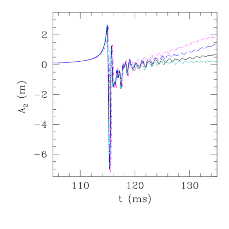
Figure 17: $A_{2}$ as a function of time for models A0 (dotted curve), A1 (dashed curve), A2 (solid curve), A3 (dot-dashed curve), and A4 (long-dashed curve).

We find that the MHD outflow modifies the gravitational waveforms in the ringdown phase; the wave amplitude gradually increases with time during this phase, although the waveforms are otherwise unchanged. That this secular increase is caused by the MHD outflow may be understood through the following simple analysis. Consider a matter outflow of mass $m$ and velocity $v$ in the $z$ direction, and assume that the velocity changes slowly. The contribution to $A_{2}$ from this outflow comes from $\ddot{I}_{zz}$, for which the correction is $\delta A_{2}\approx 2mv^{2}$. The MHD outflow is continuously ejected from the vicinity of the PNS, and hence, the total mass of the outflow increases with an approximately constant rate. We find that $A_{2}$ indeed increases roughly linearly with time. Furthermore, the magnitude is approximately given by

$$\delta A_{2}\approx 3\biggl{(}{m\over 0.1M_{\odot}}\biggr{)}\biggl{(}{v\over 0.1c}\biggr{)}^{2}~{}{\rm m},$$ (84)

which is in approximate agreement with the numerical results for the mass increase rate $dm/dt=0.1$–$5M_{\odot}$/s.

The secular increase of the wave amplitude for model A4 is faster than for model A2 although the magnetic energies of the PNSs are nearly identical. This is because the MHD outflow is more efficiently driven for model A4 as shown in Sec. VI.3.

As discussed in Sec. VI.3, the MHD outflow from a newly-formed PNS will likely hit a standing shock at a radius $\sim 150$–200 km Wilson ; Janka ; Lieb ; Burrow . The value of $m$ (and hence the linear growth of the amplitude) will then saturate in a few 10 ms. Nevertheless, the amplitude $A_{2}$ could eventually reach a few meters, which is comparable to the amplitude of the spiky waves emitted at the bounce. The outflow signal may thus be detectable for an event within our Galaxy by the ground-based laser interferometric detectors, since the expected amplitude is $\sim 10^{-20}$ [see Eq. (33)]. Detecting gravitational waves in the first few tens of ms of the supernova collapse event may thus provide information about the anisotropic outflow.

VI.6 Comparison of codes

To demonstrate agreement between the codes of DLSS and SS05 , we plot some representative quantities in Figs. 18–20. Figure 18 compares the central density evolution and late-time density profiles for model A2 from both codes. The plot of central density shows agreement on the maximum density at bounce, the slow increase in the central density caused by the spindown of the PNS, and the post-bounce oscillations (see the inset of Fig. 18). (Results from the code of DLSS were shifted forward in time by $0.35$ ms to align the core bounce. This small difference in the coordinate time likely results from the slightly different lapse prescriptions used in the two simulations.) The two codes also give the same principal features of the density profile at late times (e.g. $t=150.8$ ms), including the falloff behavior for the density outside the PNS. The behavior of the magnetic field components, as compared in Fig. 19, also shows good agreement. Some differences arise after the PNS forms due to the fact that the magnetic field evolution is dominated by the turbulent effects of the MRI. In this regime, the precise value of the maximum magnetic field component depends on the details of the turbulent motions; small differences in local quantities can be amplified by turbulence. Finally, we show the evolution of the individual components of the energy for model A2 (compare to Fig. 5), which also demonstrates good agreement between the two codes. We note that both the central density and magnetic field components grow by a factor of order $10^{4}$ during the evolution of model A2. Given this large dynamic range, the agreement shown here is rather noteworthy.

Figure 18: Results for model A2 obtained with the codes of SS05 (solid lines) and of DLSS (dotted lines). (top panel) Evolution of the central density for model A2. The inset shows the bounce and immediate post-bounce behavior. (lower panel) Comparison of the density profiles at $t=150.8$ ms. The dot-dashed line segment shows a slope of $\rho\propto\varpi^{-4}$. The results from the code of SS05 correspond to the standard resolution. For the results from the code of DLSS , a fisheye grid was used for the PNS evolution phase (see Appendix A for details).

Figure 19: Evolution of the maximum values of $|B^{i}|$ for model A2. As in Fig. 18, results from the codes of SS05 (solid lines) and of DLSS (dotted lines) are compared.

Figure 20: Individual components of the energy for model A2, defined as in Fig. 5. Results from the codes of SS05 and DLSS are shown as solid and dotted lines, respectively.

VII Summary and discussion

We have presented general relativistic numerical simulations of magnetized stellar core collapse to a PNS in axisymmetry and have followed the subsequent evolution of the PNS by magnetorotational effects. The following is a summary of the results:

1. The magnetic field is amplified during the collapse and the subsequent evolution of the PNS. During the infall phase, the poloidal field grows due to the compression of the matter in which the field is frozen. As the poloidal field strength grows, the amplification of the toroidal field by winding is accelerated. After bounce, the compression stops, and so does the rapid growth of the poloidal field. However, the differential rotation in the vicinity of the PNS induces further growth of the toroidal field through winding. The winding continues until the magnetic field drains away the kinetic energy stored in differential rotation (which is roughly 10–20% of the total rotational kinetic energy). The ratio of the magnetic energy to the rotational kinetic energy thus saturates at approximately the same value regardless of the initial magnetic field profile and strength. The poloidal magnetic field in the outer region of the PNS also grows via the MRI. In contrast to magnetic winding, the MRI amplifies the field strength in a turbulent manner. The magnetic stress increases until it becomes $\sim 10\%$ of the rotational kinetic energy density. After the magnetic field saturates, we find a stationary, collimated helical magnetic field near the rotation axis.

2. Because of the enhanced magnetic stress, an MHD outflow is launched from the vicinity of the PNS, particularly near the rotation axis. Our results suggest that three mechanisms drive the outflow. One is the magneto-spring mechanism in which magnetic stress primarily due to the toroidal field blows off matter along the rotation axis (but without strong collimation), leading to the so-called ‘tower-like’ field structure. The second mechanism is MRI-induced turbulence, which leads to a weaker and less coherent matter outflow than the magneto-spring effect. The third mechanism is the Blandford-Payne magneto-centrifugal mechanism, which plays a dominant role after the saturation of the magnetic field growth and after the formation of a collimated helical magnetic field near the rotation axis. In the present context, matter is injected into the outflow by MRI turbulence and then flung out along the helical magnetic field lines. By these three mechanisms, the energy carried away by the MHD outflow in the first 10 ms after the saturation of the toroidal magnetic field growth may be $\mathrel{\raise 1.29167pt\hbox{$>$}\mkern-14.0mu\lower 2.58334pt\hbox{$\sim$}}10^{50}$ ergs for a PNS of rotation period $\sim 1$–2 ms and for a typical ratio of the poloidal to toroidal field strength of $C_{B}\mathrel{\raise 1.29167pt\hbox{$>$}\mkern-14.0mu\lower 2.58334pt\hbox{$\sim$}}0.1$.

3: The MHD outflow carries away material with large specific angular momentum, and hence, plays a crucial role in spinning down the PNSs. We find that the angular momentum loss rate is $\sim 0.1$–$0.2E_{\rm EM}C_{B}$ as long as differential rotation persists in the vicinity of the PNS. Since $E_{\rm EM}$ is $\sim 10$–20% of the rotational kinetic energy $T_{\rm rot}$ after the field saturates, we have $|\dot{J}|\sim 0.01T_{\rm rot}C_{B}$. This implies that the angular momentum (and rotational kinetic energy) may decrease rapidly as show in Sec. VI.4. If the differential rotation remains strong enough in the first $\sim 1000$ s after the magnetic field saturates, the spin period of the PNS increases to $\mathrel{\raise 1.29167pt\hbox{$>$}\mkern-14.0mu\lower 2.58334pt\hbox{$\sim$}}1$ s.

In turbulent flows resulting from the MRI, small eddies would be formed, dissipating kinetic energy into thermal energy and transporting angular momentum outward. The thermal energy generated in this process has been suggested as a power source for a supernova explosion TQB . However, we find that the role of the turbulence is likely less important as a source of energy than the MHD outflow. This may be partly due to our choice of the initial seed magnetic field. In the present work, the poloidal magnetic field at the time of PNS formation is high enough that the toroidal field is rapidly amplified and drives a strong MHD outflow in a few tens of ms after the bounce. For a weaker initial poloidal field, more time would be required to amplify the toroidal field [see Eq. (57)] and, hence, to produce a strong MHD outflow. In contrast, the MRI grows on the same timescale ($\sim 10\Omega^{-1}$) even for very weak fields. Since the wavelength of the fastest-growing MRI mode scales with the field strength, very weak fields will result in turbulence composed of small eddies, for which the typical size is much smaller than the stellar radius. This small scale turbulence converts kinetic energy into thermal energy, as modeled in TQB . In this case, the magneto-spring and magneto-centrifugal mechanisms may not play a significant role and the collimated magnetic field may not form. Unfortunately, simulations for such weak initial fields are currently unable to capture this behavior, since the wavelength of the MRI is much too short to be resolved. To determine whether such processes indeed occur, a much more powerful supercomputer will be required.

We do not observe the magnetic field amplification mechanism found in ABM ; MBA . In this process, an MHD outflow induced by the magneto-spring mechanism is first driven along the rotation axis. This outflow then triggers convective motions, leading to the formation of large-scale eddies in the meridional plane which wind up the poloidal magnetic field lines. The strengthened poloidal field then leads to further amplification of the toroidal field. In our simulations, however, we do not find noticeable convection. The plausible reason for this discrepancy is that the simulations of ABM ; MBA use a treatment of the equation of state and microphysics, which differs from ours. In their simulations, neutrino cooling is taken into account, and this cooling leads to negative entropy gradients and subsequent convection near the neutrinosphere. In order to see this convective-type MRI MRIrev , we would have to take neutrino processes into account. This is an issue to be investigated in the future.

The simulations presented here were carried out assuming equatorial plane symmetry, and the center of the PNS thus remains at the origin. In the absence of this symmetry, the PNS may move, due to back-reaction of MHD outflows. The lack of equatorial symmetry is crucial in the explosion mechanism proposed by OBDE06 , in which acoustic waves from $l=1$ $g$-modes provide an important source of energy. In addition, the outflow may develop anisotropically, since it is driven in part by inhomogeneous MRI-induced turbulence. Anisotropic outflow could also arise if the magnetic field profile is anisotropic in the supernova progenitor. Our numerical results show that $\mathrel{\raise 1.29167pt\hbox{$>$}\mkern-14.0mu\lower 2.58334pt\hbox{$\sim$}}0.1M_{\odot}$ of material will be ejected in the first $\sim 100$ ms after the growth of the toroidal field saturates. The typical outflow velocity is $\sim 0.1c$. If the anisotropy in the direction of the ejected mass is $\mathrel{\raise 1.29167pt\hbox{$>$}\mkern-14.0mu\lower 2.58334pt\hbox{$\sim$}}10\%$, the PNS will move with a velocity $\mathrel{\raise 1.29167pt\hbox{$>$}\mkern-14.0mu\lower 2.58334pt\hbox{$\sim$}}10^{-3}c\sim 300$ km/s due to the back-reaction. Anisotropic MHD outflows may thus be able to explain high-velocity pulsars HVP . Simulations without equatorial plane symmetry would be required to explore this possibility.

An additional limitation of our simulations is the assumption of axisymmetry. Nonaxisymmetric instabilities (such as bar modes and/or one-armed spirals) may arise in the formation of PNSs and contribute strongly to the gravitational wave signal SKE ; ootb05 . In this paper, we mainly consider the case in which the progenitor is rigidly rotating and hence the resulting PNSs are weakly differentially rotating with $T_{\rm rot}/|W|\lesssim 0.12$. This implies that the PNSs found in this paper would be stable against nonaxisymmetric deformations. However, for more rapidly rotating PNSs, the possibility of nonaxisymmetric deformations have to be taken into account. The behavior of the MRI is also expected to be different in a full 3D calculation because of the effect of nonaxisymmetric MRI induced by toroidal magnetic field NMRI . Turbulence may arise and persist more readily in 3D due to the lack of symmetry. More specifically, according to the axisymmetric anti-dynamo theorem moffatt78 , sustained growth of the magnetic field energy is not possible through axisymmetric turbulence. Simulations in full 3D will eventually be necessary in order to fully understand the role of the MRI in PNS evolution and jet formation. Given current computational resources, however, we consider this a challenge for the future.

Appendix A Multiple transition fisheye coordinates

The multiple transition fisheye coordinates CLZ06 $\bar{x}^{i}$ are related to the original coordinates $x^{i}$ through the following transformation:

$$x^{i} = \frac{\bar{x}^{i}}{\bar{r}}r(\bar{r}),$$ (85)

$$r(\bar{r}) = a_{n}\bar{r}+\sum_{i=1}^{n}\kappa_{i}\ln\frac{\cosh[(\bar{r}+\bar{r}_{0i})/s_{i}]}{\cosh[(\bar{r}-\bar{r}_{0i})/s_{i}]},$$ (86)

$$\kappa_{i} = \frac{(a_{i-1}-a_{i})s_{i}}{2\tanh(\bar{r}_{0i}/s_{i})},$$ (87)

where $r=\sqrt{x^{2}+y^{2}+z^{2}}$, $\bar{r}=\sqrt{\bar{x}^{2}+\bar{y}^{2}+\bar{z}^{2}}$, $n$, $a_{i}$, $r_{0i}$ and $s_{i}$ are constant parameters. We perform simulations on this fisheye grid with $0<\bar{x}<\bar{L}$, and $0<\bar{z}<\bar{L}$. The Cartoon method is used to impose axisymmetry as usual. We use a grid size of $N\times 3\times N$ with uniform grid spacing $\bar{\Delta}=\bar{L}/N$. It follows from the transformation (85) that this corresponds to a resolution in the original grid of $\Delta\approx(dr/d\bar{r})\bar{\Delta}\approx a_{i}\bar{\Delta}$ in regions well separated from the transitions, i.e. where $\bar{r}_{0i}+s_{i}\ll\bar{r}\ll\bar{r}_{0i+1}-s_{i+1}$. The ratio $\Delta/\bar{\Delta}$ smoothly changes from $a_{i}$ to $a_{i+1}$ in the transition region $\bar{r}_{0i+1}-s_{i+1}\lesssim\bar{r}\lesssim\bar{r}_{0i+1}+s_{i+1}$.

Our implementation is as follows. We first perform simulations in the original coordinates $x^{i}$ with the regridding technique as discussed in Sec. V until the value of $\Phi_{c}$ reaches 0.16. At this time, we interpolate the data to the fisheye coordinates $\bar{x}^{i}$ with the fisheye parameters $n=3$, $(a_{0},a_{1},a_{2},a_{3})=(0.1,0.4,0.8,1.0)$. We choose the value of $\bar{L}$ so that the outer boundary is approximately the same as that of the original grid. We set $N=600$, and the values of $\bar{r}_{0i}$ so that $(r_{01},r_{02},r_{03})\approx$ (100 km, 200 km,400 km), where $r_{0i}=r(\bar{r}_{0i})$. The transition width is set to be $s_{i}=29\bar{\Delta}$. With this setting, the resulting resolution in the original grid becomes $\Delta\approx 0.7$ km for $r\lesssim 100$ km, $\Delta\approx 2.7$ km for 100 km $\lesssim r\lesssim 200$ km, $\Delta\approx 5.5$ km for 200 km $\lesssim r\lesssim 400$ km, and $\Delta\approx 6.8$ km for $r\gtrsim 400$ km. Therefore, using this technique, we can achieve high resolution in the central region with relatively few grid points.

Appendix B Proof of $k=\rho_{*}v^{P}/{\cal{B}}^{P}$ constant along magnetic field lines

In a stationary spacetime, $\partial_{t}{\cal{B}}^{i}=0=\partial_{t}\rho_{*}$. It follows from the induction equation (36) and the continuity equation (37) that

$$\partial_{j}(v^{j}{\cal{B}}^{i}-v^{i}{\cal{B}}^{j}) = 0,$$ (88)

$$\partial_{j}(\rho_{*}v^{j}) = 0.$$ (89)

In an axisymmetric spacetime, the continuity equation becomes

$$\partial_{P}(\varpi\rho_{*}v^{P})=0,$$ (90)

where $P$ denotes the poloidal components ($\varpi$ and $z$). We introduce a one-form

$$\omega_{i}=\epsilon_{ijk}v^{j}B^{k}=[ijk]v^{j}{\cal{B}}^{k},$$ (91)

where $\epsilon_{\alpha\beta\gamma}=n^{\mu}\epsilon_{\mu\alpha\beta\gamma}$ is the 3-dimensional Levi-Civita tensor, and $[ijk]$ is the permutation symbol. It is easy to show that Eq. (88) is equivalent to $D_{[i}\omega_{j]}=0$ (i.e. $\omega_{i}$ is a closed one-form), where $D_{i}$ denotes the covariant derivative associated with the three-metric $\gamma_{ij}$. Hence $\omega_{i}$ can be written as

$$\omega_{i}=D_{i}f=\partial_{i}f,$$ (92)

where $f$ is a scalar function. We assume that Eq. (92) holds globally. It follows that $\omega_{\varphi}=\varpi(v^{z}{\cal{B}}^{\varpi}-v^{\varpi}{\cal{B}}^{z})=0$ in an axisymmetric and stationary spacetime. This implies that $v^{\varpi}/{\cal{B}}^{\varpi}=v^{z}/{\cal{B}}^{z}$, i.e. $v^{P}=\mu{\cal{B}}^{P}$, where $\mu$ is a scalar function. Substituting $v^{P}=\mu{\cal{B}}^{P}$ into Eq. (90) we have $\partial_{P}(\varpi\rho_{*}\mu{\cal{B}}^{P})=0$. Using the no-monopole constraint $\partial_{P}(\varpi{\cal{B}}^{P})=0$, we obtain $B^{P}\partial_{P}k=0=B^{j}\partial_{j}k$, where $k\equiv\rho_{*}\mu=\rho_{*}v^{P}/{\cal{B}}^{P}$. Hence $k$ is constant along magnetic field lines in an axisymmetric, stationary spacetime.

References

- (1) S. Woosley and T. Janka, Nature Physics 1, 147 (2005).
- (2) A. Burrows, E. Livne, L. Dessart, C. D. Ott, and J. Murphy, Astrophys. J. 640, 878 (2006); C. D. Ott, A. Burrows, L. Dessart, E. Livne, Phys. Rev. Lett., 96, 201102 (2006).
- (3) P. M. Woods and C. Thompson, in Compact Stellar X-ray Sources, edited by W. H. G. Lewin and M. van der Klis (Cambridge University Press, 2006)
- (4) C. Thompson and R. C. Duncan, Mon. Not. R. Astro. Soc. 275, 255 (1995); Astrophys. J. 473, 322 (1996).
- (5) R. C. Duncan and C. Thompson, Astrophys. J. 392, L9 (1992).
- (6) J. C. Wheeler, D. L. Meier, and . J. R. Wilson, Astrophys. J. 568, 807 (2002).
- (7) S. Akiyama, J. C. Wheeler, D. L. Meier, and I. Lichtenstadt, Astrophys. J. 584, 954 (2003).
- (8) T. A. Thompson, P.Chang, and E. Quataert, Astrophys. J. 611, 380 (2004).
- (9) T. A. Thompson, E. Quataert, and A. Burrows, Astrophys. J. 620, 861 (2005).
- (10) L. Spitzer, Jr., Physical Processes in the Interstellar Medium (John Wiley, New York, 1978).
- (11) H. C. Spruit, Astron. and Astrophys., 349, 189 (1999)
- (12) T. W. Baumgarte, S. L. Shapiro, and M. Shibata, Astrophys. J. Lett. 528, L29 (2000).
- (13) S. L. Shapiro, Astrophys. J. 544, 397 (2000); J. N. Cook, S. L. Shapiro, and B. C. Stephens, Astrophys. J. 599, 1272 (2003); Y. T. Liu and S. L. Shapiro, Phys. Rev. D, 69, 104030 (2004).
- (14) V. P. Velikhov, Soc. Phys. JETP, 36, 995 (1959); S. Chandrasekhar, Proc. Natl. Acad. Sci. USA, 46, 253 (1960).
- (15) S. A. Balbus and J. F. Hawley, Astrophys. J. 376, 214 (1991)
- (16) S. A. Balbus and J. F. Hawley, Rev. Mod. Phys. 70, 1 (1998).
- (17) J. L. Friedman, J. R. Ipser, and L. Parker, Astrophys. J. 304, 115 (1986).
- (18) G. C. Cook, S. L. Shapiro, and S. A. Teukolsky, Astrophys. J. 422, 227 (1994).
- (19) J. M. LeBlanc and J. R. Wilson, Astrophys. J. 191, 541 (1970).
- (20) E. M. D. Symbalisty, Astrophys. J. 285, 729 (1984).
- (21) S. Yamada and H. Sawai, Astrophys. J. 608, 907 (2004).
- (22) H. Sawai, K. Kotake, and S. Yamada, Astrophys. J. 631, 446 (2005).
- (23) T. Takiwaki, K. Kotake, S. Nagataki, and K. Sato, Astrophys. J. 616, 1086 (2004).
- (24) K. Kotake, H. Sawai, S. Yamada, and K. Sato, Astrophys. J. 608, 391 (2004).
- (25) M. Obergaulinger, M. A. Aloy, and E. Müller, Astron. Astrophys., 450, 1107 (2006).
- (26) M. Obergaulinger, M. A. Aloy, H. Dimmelmeier, and E. Müller, submitted to Astron. Astrophys. (astro-ph/0602187).
- (27) N. V. Adreljan, G. S. Bisnobatyi-Kogan, and S. G. Moiseenko, Mon. Not. R. Astro. Soc. 359, 333 (2005).
- (28) S. G. Moiseenko, G. S. Bisnobatyi-Kogan, and N. V. Adreljan, astro-ph/0603789.
- (29) In the work of YS ; SKY ; OAM , a logarithmic grid spacing is adopted for the radial coordinate and a sufficient resolution was guaranteed only in the central region. However, the MRI is active not at the central region, but near the surface of the PNS. The wavelength of the fastest-growing mode of the MRI is proportional to the strength of the poloidal magnetic field (see Sec. III.3). The simulation of OAM can resolve it in the strongest magnetic strength. However, in this case, other MHD effects dominate and it is difficult to identify the role of the MRI as mentioned in OAM . On the other hand, for the weaker magnetic field strength, they could not resolve the MRI because of insufficient grid resolution.
- (30) M. D. Duez, Y. T. Liu, S. L. Shapiro, and B. C. Stephens, Phys. Rev. D 72, 024028 (2005).
- (31) M. Shibata and Y.-I. Sekiguchi, Phys. Rev. D 72, 044014 (2005).
- (32) M. D. Duez, Y. T. Liu, S. L. Shapiro, M. Shibata, and B. C. Stephens, Phys. Rev. Lett. 96, 031101 (2006); M. Shibata, M. D. Duez, Y. T. Liu, S. L. Shapiro, and B. C. Stephens, Phys. Rev. Lett. 96, 031102 (2006).
- (33) M. D. Duez, Y. T. Liu, S. L. Shapiro, M. Shibata, and B. C. Stephens, Phys. Rev. D, 73, 104015 (2006).
- (34) M. Campanelli, C. O. Lousto, and Y. Zlochower, Phys. Rev. D, 73 061501 (2006).
- (35) A. Heger, S. E. Woosley, and H. C. Spruit, Astrophys. J. 626, 350 (2005).
- (36) M. Shibata and T. Nakamura, Phys. Rev. D 52, 5428 (1995).
- (37) M. Shibata, Prog. Theor. Phys. 101, 1199 (1999).
- (38) T. W. Baumgarte and S. L. Shapiro, Phys. Rev. D 59 (1999), 024007.
- (39) M. Alcubierre et al., Phys. Rev. D 61 (2000), 041501.
- (40) M. Shibata and K. Uryū, Prog. Theor. Phys. 107, 265 (2002).
- (41) M. Alcubierre, S. Brandt, B. Brügmann, D. Holz, E. Seidel, R. Takahashi and J. Thornburg, Int. J. Mod. Phys. D 10, 273 (2001).
- (42) M. Shibata, Phys. Rev. D 67, 024033 (2003).
- (43) M. Shibata, Phys. Rev. D 60, 104052 (1999).
- (44) M. Shibata, Astrophys. J. 595, 992 (2003).
- (45) M. Shibata, K. Taniguchi, and K. Uryū, Phys. Rev. D 68, 084020 (2003).
- (46) M. D. Duez, S. L. Shapiro, and H.-J. Yo, Phys. Rev. D 69, 104016 (2004).
- (47) A. Kurganov and E. Tadmor, J. Comput. Phys. 160, 214 (2000).
- (48) M. Shibata and J. A. Font, Phys. Rev. D 72, 047501 (2005).
- (49) A. Harten, P. D. Lax, and B. J. van Leer, SIAM Rev. 25, 35 (1983).
- (50) B. J. van Leer, J. Comput. Phys. 23, 276 (1977).
- (51) L. Antón, O. Zanotti, J. A. Miralles, J. M. Martí, J. M. Ibáñez, J. A. Font, and J. A. Pons, Astrophys. J. 637, 296 (2006).
- (52) J. A. Font, Living Rev. Relativ. 6, 4 (2003).
- (53) C. R. Evans and J. F. Hawley, Astrophys. J. 332, 659 (1988).
- (54) G. Tóth, J. Comput. Phys. 161, 605 (2000); C.F. Gammie, J.C. McKinney, and G. Tóth, Astrophys. J. 589, 444 (2003).
- (55) T. Zwerger and E. Müller, Astron. Astrophys. 320, 209 (1997).
- (56) H. Dimmelmeier, J. A. Font and E. Müller, Astro. Astrophys. 388, 917 (2002); 393, 523 (2002).
- (57) e.g., S. L. Shapiro and S. A. Teukolsky, Black Holes, White Dwarfs, and Neutron Stars, Wiley Interscience (New York, 1983).
- (58) M. Shibata and Y.-I. Sekiguchi, Phys. Rev. D 68, 104020 (2003).
- (59) M. Shibata and Y.-I. Sekiguchi, Phys. Rev. D 69, 084024 (2004).
- (60) H. Komatsu, Y. Eriguchi, and I. Hachisu, Mon. Not. R. Astron. Soc., 237, 355 (1989); 239, 153 (1989).
- (61) N. Stergioulas, Living Rev. Relativ, 1, 8 (1998).
- (62) M. Shibata and S. L. Shapiro, Astrophys. J. Lett. 572, L39 (2002).
- (63) Y. Uchida and K. Shibata, Pub. Astro. Soc. J. 37, 515 (1985).
- (64) Y. Kato, M. R. Hayashi, and R. Matsumoto, Astrophys. J. 600, 338 (2004).
- (65) M.M. Romanova, G. V. Ustyugova, A. V. K. Koldoba, and R. V. E. Lovelace, Astrophys. J. 635, L165 (2005).
- (66) R. D. Blandford and D. G. Payne, Mon. Not. R. Astro. Soc. 199, 883 (1982).
- (67) G. V. Ustyugova, A. V. Koldoba, M. M. Romanova, V. M. Chechetkin, and R. V. E. Lovelace, Astrophys. J. 516, 221 (1999).
- (68) R. Krasnopolsky, Z-Y. Li, and R. Blandford, Astrophys. J. 526, 631 (1999); 595, 631 (2003).
- (69) In a real supernova, the shock will stall at a radius of –200 km forming a standing shock Wilson ; Janka ; Lieb ; Burrow . In this paper, we do not pay attention to the issue for the propagation of the shock and longterm dynamics of supernova explosion.
- (70) J. R. Wilson, in Numerical astrophysics, editted by J. M. Centrella, J. M. LeBlanc, and R. L. Bowers (Boston, Jones and Bartlett, 1985), 422; H. A. Bethe and J. R. Wilson, Astrophys. J. 295, 14 (1985).
- (71) M. Rampp and H.-T. Janka, Astrophys. J. 539, L33 (2000); Astronomy and Astrophys. 396, 361 (2002).
- (72) M. Liebendörfer et al., Astrophys. J. Suppl. 150, 263 (2004).
- (73) A. Burrows, T. Young, P. Pinto, R. Eastman, and T. A. Thompson, Astrophys. J. 539, 865 (2000); A. Burrows, E. Livne, L. Dessart, C. D. Ott, and J. Murphy, Astrohpys. J. 640, 878 (2006).
- (74) E. N. Parker, Astrophys. J. 180, 247 (1973)
- (75) E. R. Priest and A. M. Soward, in Proceedings of the IAU Symposium No. 71, Prague, 1975, edited by V. Bumba and J. Kleczek (D. Reidel, Boston, 1976), p. 353.
- (76) R. M. Kulsrud, Plasma Physics for Astrophysics (Princeton University Press, 2005).
- (77) This feature is clearly seen in the animation for the evolution of the magnetic field lines and matter motion: http://esa.c.u-tokyo.ac.jp/shibata/can5m.mpg.
- (78) C. Curry, R. E. Pudritz, and P. G. Sutherland, Astrophys. J. 434, 206 (1994).
- (79) L. Mestel, Mon. Not. R. Astro. Soc. 138, 359 (1968).
- (80) Note that the fact does not imply that approximately all the energy are carried away by the Poynting flux since is composed of the bulk kinetic, thermal, rotational kinetic, electromagnetic, and gravitational potential energy. The last one is negative and decreases the value of . Thus, implies that absolute value of the gravitational potential energy is nearly equal to the sum of the bulk kinetic, thermal, and rotational kinetic energy.
- (81) A. Lyne and F. Graham-Smith, Pulsar Astronomy, third edition (Cambridge University Press, Cambridge, 2006).
- (82) G. Hobbs, D. R. Lorimer, A. G. Lyne, and M. Kramer, Mon. Not. R. Astro. Soc. 360, 963 (2005).
- (83) M. Shibata, S. Karino, and Y. Eriguchi, Mon. Not. R. Astro. Soc. 334, L27 (2002): M. Shibata and Y. Sekiguchi, Phys. Rev. D 71, 024014 (2005).
- (84) C. D. Ott, S. Ou, J. E. Tohline, and A. Burrows, Astrophys. J. Lett. 625, 119 (2005).
- (85) C. Terquem and J. C. B. Papaloizou, Mon. Not. R. Astro. Soc. 279, 767 (2996); C. Curry and R. E. Pudritz, Mon. Not. R. Astro. Soc. 281, 119 (1996); Y. Masada, T. Sano, and H. Takabe, Astrophys. J. 641, 447 (2006).
- (86) H. K. Moffatt, Magnetic Field Generation in Electrically Conducting Fluids (Cambridge Univ. Press, 1978).