Search for Gravitational Waves in the CMB After WMAP3: Foreground Confusion and The Optimal Frequency Coverage for Foreground Minimization

Abstract

B-modes of Cosmic Microwave Background (CMB) polarization can be created by a primordial gravitational wave background. If this background was created by Inflation, then the amplitude of the polarization signal is proportional the energy density of the universe during inflation. The primordial signal will be contaminated by polarized foregrounds including dust and synchrotron emission within the galaxy. In light of the WMAP polarization maps, we consider the ability of several hypothetical CMB polarization experiments to separate primordial CMB B-mode signal from galactic foregrounds. We also study the optimization of a CMB experiment with a fixed number of detectors in the focal plane to determine how the detectors should be distributed in different frequency bands to minimize foreground confusion. We show that the optimal configuration requires observations in at least 5 channels spread over the frequency range between 30 GHz and 500 GHz with substantial coverage around 150 GHz. If a low-resolution space experiment using 1000 detectors to reach a noise level of about 1000 nK² concentrates on roughly 66% of the sky with the least foreground contamination the minimum detectable level of the tensor-to-scalar ratio would be about 0.002 at the 99% confidence level for an optical depth of 0.1.

I Introduction

The cosmic microwave background (CMB) is a well known probe of the early universe. The acoustic peaks in the angular power spectrum of CMB anisotropies capture the physics of the primordial photon-baryon fluid undergoing oscillations in the potential wells of dark matter Huetal97 . The associated physics involving the evolution of a single photon-baryon fluid under Compton scattering and gravity is both simple and linear SacWol67 ; Sil68 ; PeeYu70 ; SunZel70 .

The acoustic peak structure has been well established with the Wilkinson Microwave Anisotropy Probe (WMAP; Hinetal06 ; Speetal06 ) data. Over the next several years, with the launch of the ESA’s Planck surveyor, it is expected that the anisotropy power spectrum will be measured to the cosmic variance limit out to an angular scale of roughly ten arcminutes (or multipoles $\sim$ 2000 in the angular power spectrum; see, review in HuDod02 ).

Beyond temperature anisotropies, the focus is now on the polarization at medium to larger angular scales. When the Universe was reionized, the temperature quadrupole rescattered at the reionization surface producing a new contribution to the polarization Zal97 . Such a signature has now been detected in the WMAP data Pagetal06 ; Speetal06 . Furthermore, the CMB polarization field contains a signature of primordial gravitational waves, which is considered a smoking-gun signature for inflation as models of inflation predict a stochastic gravitational wave background in addition to the density perturbation spectrum Starobinsky79 ; KamKos99 . The distinct signature is in the form of a curl component, also called B-mode, of the two-dimensional polarization field Kametal97 ; SelZal97 .

Observation of the primordial B-modes is now the primary goal of a large number of ground- and balloon-borne CMB polarization experiments. There are also plans for a next generation CMB polarization mission as part of NASA’s Beyond Einstein program (Inflation Probe). The only known source for primordial B-modes is inflationary gravitational waves (IGWs) and a detection of this tensor component would be one of the biggest discoveries in science. The tensor component captures important physics related to the inflaton potential, especially the energy scale at which relevant models exit the horizon KamKos99 .

CMB polarization observations are significantly impacted by foreground polarized radiation, with initial estimates suggesting that the minimum amplitude to which a gravitational wave background can be searched is not significantly below a tensor-to-scalar ratio of 10^-3 Verde06 ; Amarie:2005in ; Carretti:2006us . This limit based on analysis of foregrounds is well above the ultimate limit of a tensor-to-scalar ratio around $10^{-4}$ due to the cosmic shear confusion, associated with secondary B-modes generated from E-modes by lensing due to intervening structure Kesden ; Song ; Seljak:2003pn . If the optical depth is around 0.1, then the ultimate limit may be pushed down an order of magnitude KapKnoSon03 by measuring the large angle B mode polarization signal.

While the impact of foregrounds is now well appreciated, it is not fully clear how these foregrounds may be minimized in the next generation experiments. This issue critically impacts the planning of experiments. For the Inflation Probe or a ground-based experiment that attempts to target the gravitational wave background, one of the most significant issues to address is the choice of frequency bands for observations such that the foreground contamination is minimized. For example, should an experiment target the low-frequency end where synchrotron dominates, high-frequency end where dust dominates, or the frequency range between 50 GHz to 100 GHz where foreground polarization is minimum, but contributions from both synchrotron and dust are expected? We find that frequency bands over a wide range from low frequencies dominated by synchrotron to high frequencies dominated by dust are required. Furthermore, we also study the optimization problem of dividing a fixed number of detectors in the focal plane among the frequency bands. We looked into the question of whether the division should be such that one has equal noise in each band or whether we should concentrate more detectors in channels where foreground components dominate.

To address the issue of foreground contamination and the optimization necessary to minimize foregrounds, we made use of the recently released WMAP polarization data Pagetal06 . The WMAP data has provided us with an estimate of the polarized synchrotron foregrounds at low frequencies. For dust polarization, we also made use of dust maps from Ref. SFD98 . We considered several different experimental possibilities with frequency coverages either at the high-end or low-end of our frequency range as well as an experiment with several channels that cover the range from 30 GHz to 300 GHz.

The paper is organized in the following manner. In the next section, we will discuss the simulated maps, summarize the foreground model and discuss the foreground removal method employed. In Section 3, we will discuss contamination in example CMB experiments with two or more frequency bands spread over the broad range from 30 GHz to 300 GHz. In Section 4, we will consider the optimization of experiments such as Inflation Probe. Here optimization refers to the selection of frequency bands with total number of detectors kept fixed so as to minimize foreground confusion. We discuss our results and conclude with a summary in Section 5.

Our main results are two-fold. First, we quantify the effect of foregrounds on experiments with different frequency coverages and the improved sensitivity to B modes from adding future WMAP or Planck data. Our results from this study are summarized in Table 2. The second result concerns the optimal spacing of frequency bands for a CMB experiment that aims to detect primordial B-modes. We discuss the optimization in § III while our results are summarized in Table 3.

Expt.1	Frequencies	NET2	angular resolution	fsky	Tobs
	(GHz)	($\mu$K$\sqrt{\rm sec}$)	(arcmins)		(days)
A	45, 75, 85, 100, 145, 165	13.0, 6.0, 5.6, 6.2, 5.0, 5.5	115.2, 69.1, 60.4, 52.4, 36.0, 32.0	45% (34%)	10
B	100, 150, 220	9.8, 10.4, 35.2	55, 37, 26	2.5%	600
C	40, 90	18, 9	16, 7	3%	1000
D	40, 60, 90 135, 200, 300	12.0, 7.1, 3.4 2.7, 2.7, 3.4	116, 77.5, 52.0 34.5, 23.0, 15.5	100% (13%)	730

Table 1: Example CMB polarization experiments used for the foreground analysis and their specifications in terms of the experimental noise, angular resolution and the sky area observed.
Notes: —
¹: Experiments B and C are typical of ground-based experiments that target a small area on the sky with limited frequencies and concentrating on either low- or high-frequencies. Experiment A is an example of a balloon-borne experiment with a large sky coverage. Note that the sky area observed is 45% but we assume that a smaller area (34%) is clean enough for CMB measurements. Experiment D is consistent (same as A, 100% observed but 13% used) with one of the concept study designs of the Inflation Probe mission for high precision CMB polarization measurements.
²: The NET (noise-equivalent-temperature) in units of $\mu$K$\sqrt{\rm sec}$ is the focal plane sensitivity at each of the channels. This is equivalent to the NET of a single detector divided by the square-root of the number of detectors.

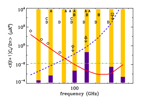
Figure 1: Dust (blue dashed line), Synchrotron (red solid line) and CMB (green dotted-dashed line) spectrum estimated with our model in thermodynamic units (in $\mu$K²). The ordinate is the average of C_ℓ($\ell$+1)$\ell$/2$\pi$ over $10<\ell<100$. The channels marked with letters A, B, C, D show different experiments studied. These channel selections represent some of the choices considered by ongoing and planned experiments in the field. Using height as a representation of the number of detectors, the lower bars show the optimal experiment that minimizes foregrounds and maximizes the detectability of primordial tensors in the B-mode polarization power spectrum. The optimization involved a priori selection of 8 channels shown here and a fixed number of detectors in the focal plane. The 150 GHz channel with the largest number of detectors provide high sensitive CMB observations, while the low- and high-frequency bands monitor the synchrotron and dust foregrounds, respectively. The achievable tensor-to-scalar ratio in the optimized setup is on average 36% better without lensing and 20% better with lensing, than the case where all detectors are spread equally among the 8 channels. The foreground residual is in both cases smaller by roughly a factor of two. The diamond, triangle and square represent the B-mode measurement or 2-$\sigma$ upper limit (with the down arrow) of WMAP (value at $\ell=5$ Pagetal06 ), Boomerang (value between $\ell$ of 201 and 1000, Monetal06 ) and Archeops (value between $\ell$ of 20 and 70 Ponetal05 ). The comparison between these measurements and our spectra is to be treated with caution since the scales ($\ell$ range) and the sky coverage do not always match.

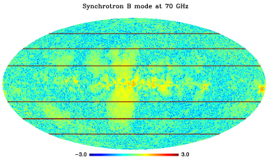
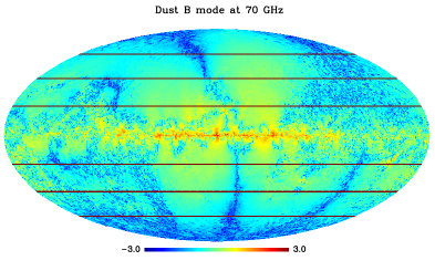
Figure 2: B-mode maps of the synchrotron (right) and dust (left) emission at 70 GHz, the scale is logarithmic going from 10^-3 $\mu$K to 10³ $\mu$K. The 6 horizontal lines represent the galactic latitude at -60, -40, -20, 20, 40 and 60 degrees. We used only the part of the map outside the galactic plane ($|$ galactic latitude$|>$20), which represents 65.8% of the sky. For some of the experiments we discuss here, we also considered smaller sky coverages from 2.5% to 45%. In these cases, we assumed that the experiments will target a low, but not necessarily the lowest, foreground emission sky area for observations.

II Impact of Foregrounds on B-mode Measurements

II.1 Models of dust and synchrotron polarization

We have included the new polarized data from WMAP at 23 GHz Pagetal06 ; Hinetal06 in our simulations. These observations form the core of our calculations. We assume the WMAP 23 GHz channel is dominated by synchrotron emission. To avoid excess noise at smallest angular scales probed by WMAP at 23 GHz, we filter the maps at multipoles more than 40 and extrapolate the synchrotron power spectrum out to a multipole of 200 using the same power-law slope for synchrotron power spectrum with multipole at $\ell<40$. For synchrotron emission at higher frequencies, we extrapolated this map using the software provided by the WOMBAT project . The WOMBAT project uses the spectral index $\beta$ obtained from combining the Rhodes/HartRAO 2326 MHz survey Jonetal98 , the Stockert 21cm radio continuum survey at 1420 MHz Rei82 ; ReiRei86 , and the all-sky 408 MHz survey Hasetal81 .

In our extrapolation, we assumed that the spectral index varies across the sky (down to about 1 degree) but is constant over the range of frequencies considered. There is, however, an indication in the WMAP data that the synchrotron spectral index is decreasing with increasing frequency Hinetal06 ; Pagetal06 , but it is not yet established whether this is real or a reflection of the increasing dust contribution at higher frequencies.

In order to simulate the dust polarization, we again made use of the WMAP 23 GHz map by assuming that the synchrotron signal is a good tracer of the galactic magnetic field and that the dust grains align very efficiently with this magnetic field. We used the synchrotron polarization angle to describe the dust polarization as well, consistent with the model presented by Ref. Pagetal06 to describe the galactic synchrotron map. For the intensity, we crudely assumed a constant overall polarization fraction of 5% relative to the total dust intensity at a given frequency. Such a fraction is consistent with most recent measurements of dust polarization outside the galactic plane such as Archeops experiment at 353 GHz Ponetal05 , and with theoretical models Mar06 . Using this fraction, we again used the interpolation of model 8 of Ref. Finetal99 of the maps from Ref. SFD98 to simulate the polarized dust emission over the frequency range of 30 GHz to 300 GHz.

In the present work, we consider polarized foregrounds due dust and synchrotron emission. Free-free emission contributes to intensity anisotropies but is unpolarized. A third component in polarization maps may come from the spinning dust. Relative to the total intensity of the spinning dust background, the polarized fraction is about 5% at a few GHz but below 0.5% at frequencies around 30 GHz, where CMB observations begin LazDra00 . There is no evidence for a spinning dust component in WMAP polarization data Pagetal06 , but this is perhaps susceptible to model uncertainties.

Following the above guidelines, we simulated the synchrotron, dust and CMB signals. We assumed a standard $\Lambda$CDM cosmological model in agreement with WMAP recent results Speetal06 . The simulated synchrotron and dust map were produced in the HEALPix pixelization scheme. When plotting our results, for comparison, we also plot the power spectrum of the B-mode tensor component assuming a tensor-to-scalar ratio $r$ of 0.3. When we present our results, however, we will discuss the minimum amplitude of the tensor component that experiments will be able to detect given the presence of residual foregrounds. We plot example frequency maps as well as spectra in Figs. 2 & 3.

Our maps generate power spectra that match the values obtained from WMAP data Pagetal06 for the synchrotron polarization with rms fluctuations at the level of $\simeq$ 25, 5, 2, 1 $\mu$K² at 23, 33, 40, 61 GHz between $\ell$ of 2 and 100. In terms of dust, our maps and the resulting power spectra are again consistent with CMB measurements at high frequencies: Boomerang data provide a limit of 8.6 $\mu$K² at 145 GHz for average fluctuations at $201<\ell<1000$ Monetal06 while Archeops data Ponetal05 lead to a limit of 2200 $\mu$K² at 353 GHz over $20<\ell<70$ (both at 2 $\sigma$ confidence level). These limits are consistent with the maximal level of dust in areas corresponding to these observations.

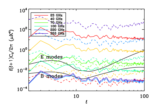
Figure 3: Dust (dashed lines) and synchrotron (solid lines) power spectra at six frequencies between 23 and 353 GHz (from red to purple) as labeled on the figure. For comparison, we plotted the primordial E-mode and B-mode CMB power spectra consistent with WMAP3 and assuming $r=0.3$.

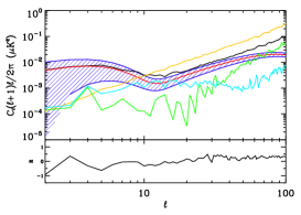
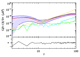
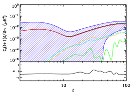
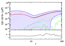
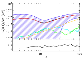
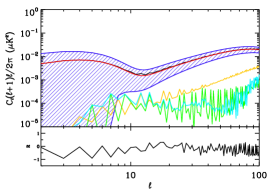
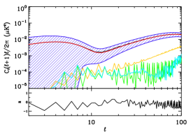
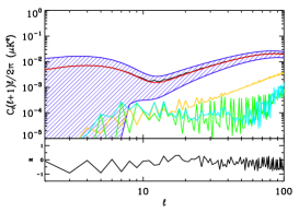
Figure 4: Residual B-mode power spectra for experiments discussed in Table 1. We show the total residual power spectrum (black), dust residual (green), synchrotron residual (blue), and detector noise (orange). The red curve is the primordial B-mode power spectrum with $r=0.3$. From top to bottom in each of the rows, the experiments are A to D, respectively. The first (left) column shows the residual with data from each of the experiments alone, the middle column is for the experiments combined with 8-year data from WMAP, and the third (right) column is for the experiments combined with 14-month data from Planck. R, at the bottom of each plot, is the cross-correlation of dust and synchrotron residuals divided by the sum of the auto-correlations of dust and synchrotron residuals.

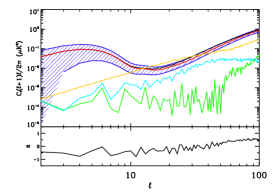
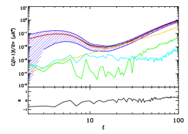
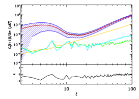
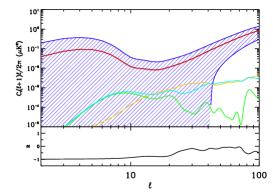
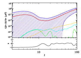
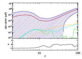
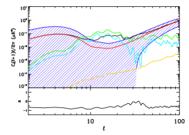
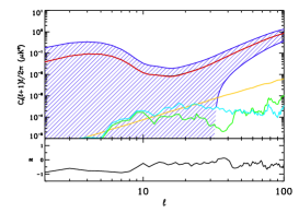
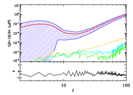
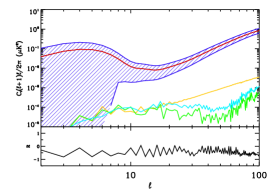
Figure 5: Residual E-mode power spectra for experiments discussed in Table 1. The curve labels and the panel layout are same as Figure 4.

II.2 CMB Polarization Experiments

We considered hypothetical current and future generation CMB experiments, and simulated maps for these experiments by adding the appropriate noise. Table 1 lists our example experiments. We included experiments that target the low frequency range (where synchrotron polarization dominates), the high frequency range (where dust dominates), and possibilities that span across the frequency range from 30 GHz to 300 GHz. Two of the experiments are based on ground-based attempts to detect primordial B-modes by targeting a small clean area on the sky (experiments B and C), one suborbital balloon-borne experiment (experiment A), and another based on a mission concept for the NASA Inflation Probe. Table 1 lists the frequency bands, the focal-plane sensitivity at each of the frequency bands, angular resolution assuming a fixed aperture size, the fraction of sky covered and the duration of the experiment.

When converting simulated foreground and CMB maps to observable maps, we made certain simplifications. For example, we did not simulate a scan pattern on the sky but instead added instrumental noise as white noise to the maps with uniform sensitivity across the observed area. In particular in this procedure, we do not account for systematics such as side-lobes and cross-talks between different modes associated with non-Gaussian beam shapes HuZal . Our aim here is to estimate the effect of our current knowledge about polarized foregrounds. Once this issue is better understood we can address systematics such as those associated with side-lobes and beam shapes.

Our maps are decomposed perfectly to E and B components. In practice, for partial sky coverage, decomposition of Q and U (Stokes parameters) maps to E and B polarization modes will lead to mixing between the E and B modes Bunn . This mixing, however, can be reduced through optimized estimators Smith and since these problems are not exacerbated by foregrounds, we have ignored the added complication in this study.

II.3 Foreground removal technique

In order to study how well simulated maps for each experiment can be used to remove foregrounds, we used the cleaning technique outlined in Ref. Tegetal03 , where multifrequency maps from WMAP first-year data were used to produce the so-called TOH foreground-cleaned CMB map. This technique allows to take into account the variation of the spectral index in real space and is more efficient at removing foregrounds than a simple model with a constant coefficient for the whole map (all the mode $\ell$) even on small part of the sky like experiment B coverage (2.36 % of the sky). When comparing the residual foreground for a simple coefficient model to the one obtained by Tegmark et al. Tegetal03 algorithm, we found that the latter improved the residual foreground level by a factor 5 for experiment B (see figure 6).

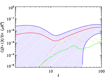
Figure 6: Residual foregrounds obtained using a constant coefficient for the whole map (dashed orange line) and using the Tegetal03 algorithm with one coefficient per $\ell$ mode (solide green line) for the experiment B setup. The red solid line represents the theoretical CMB power spectrum for r=0.3 and the blue hatched area the cosmic variance for the experiment B setup.

Therefore we restrain ourselves in the rest of this paper to the Tegmark et al. Tegetal03 foreground cleaning technique. The technique recommends taking a linear combination of observed $a_{\ell m}$’s in each frequency band $i$,

$$a_{\ell m}=\sum_{freq=i}w^{i}_{\ell}a^{i}_{\ell m}\,.$$ (1)

The weights $w_{i}$ are then to be chosen to minimize foreground contamination. For polarized observations, we can decompose the signal at each frequency as

$$a^{i}_{\ell m}=c_{\ell m}+s^{i}_{\ell m}+d^{i}_{\ell m}+n^{i}_{\ell m}\,,$$ (2)

where $c$, $s$, $d$, and $n$ stand respectively for the CMB, synchrotron, dust, and noise. We then minimize the resulting power spectrum

$$\langle|a_{\ell m}|^{2}\rangle={\bf w_{\ell}}^{T}{\cal C}{\bf w_{\ell}}\,,$$ (3)

with respect to the weights under the constraint $w_{\ell}^{T}\cdot{\bf e}=1$, when ${\bf e}$ is a column vector of all ones with length equal to the number of channels. This condition ensures that the CMB signal is unchanged regardless of the chosen weights. Here, ${\cal C}^{ij}_{\ell}$ matrix represents $\langle(a^{i}_{\ell m})^{\dagger}a^{j}_{\ell m}\rangle$. As derived in Ref. Tegetal03 , the weights that minimize the power $\langle|a_{\ell m}|^{2}\rangle$ are

$${\bf w_{\ell}}=\frac{{\cal C}^{-1}{\bf e}}{e^{T}{\cal C}^{-1}e}\,.$$ (4)

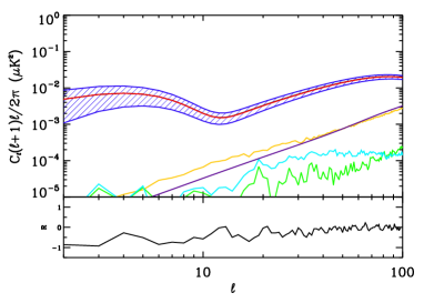
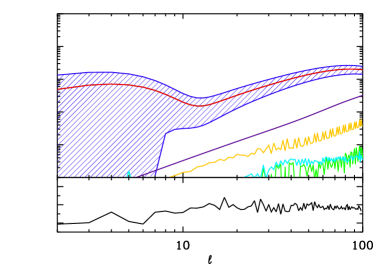
Figure 7: Estimated B mode power spectrum (solid black line) for a 1000 detector “optimized” experiment covering 65.8, 35.7, 13.4 %7b of the sky. The green and light blue solid lines correspond respectively to the residual dust and synchrotron, the orange solid line represent the noise power spectrum, the red solid line the theoretical CMB power spectrum (WMAP cosmological parameters and r=0.3), and the blue hatched area correspond to the cosmic variance. R, at the bottom of each plot, is the cross-correlation of dust and synchrotron residuals divided by the sum of the auto-correlations of dust and synchrotron residuals.

II.4 Minimal Tensor-to-Scalar Ratio

For each of the experiments, we compute four quantities to test the level of residual foreground and detector noise in the cleaned map, and the achievable lower limit on the tensor-to-scalar ratio $r$, which we quote as a 3 $\sigma$ confidence limit.

1. Average noise power in the map (where $N_{\ell}$ is the noise power spectrum) between $\ell$ of 2 and 100 :

$$\mathrm{av\_noise}=\frac{1}{99}\sum_{\ell=2}^{100}{{N_{\ell}(\ell+1)\ell\over 2\pi}}\,.$$ (5)

2. Average noise power spectrum variance of the map between $\ell$ of 2 and 100 :

$$\mathrm{av\_noise\_var}=\frac{1}{99}\sum_{\ell=2}^{100}{{N_{\ell}(\ell+1)\ell\over 2\pi}\sqrt{2\over(2\ell+1)f_{sky}}}\,.$$ (6)

3. Average residual in the estimated power spectrum of the map after subtracting the CMB and noise power spectrum between $\ell$ of 2 and 100:

$$\mathrm{av\_fgd\_var}=\frac{1}{99}\sum_{\ell=2}^{100}{{R_{\ell}(\ell+1)\ell\over 2\pi}}\,.$$ (7)

4. $r_{g}$, “Gaussian” estimate of achievable tensor to scalar ratio, the foreground residual $R_{\ell}$ is assumed to be an extra Gaussian noise and we sum over all the $\ell$ modes optimally to constrain the overall signal-to-noise ratio to be above 3 for $r_{g}$ :

$$\sqrt{\sum_{\ell=\ell_{min}}^{\ell=\ell_{max}}\left(C_{\ell}(r_{g})\over(R_{\ell}+(N_{\ell}+C_{\ell}(r_{g}))\sqrt{2\over(2\ell+1)f_{sky}})\right)^{2}}=3$$ (8)

When not specified, $\ell_{\rm min}$ is given by the largest mode that fits within the sky area observed by a given experiment, or $\pi/\theta$, where $\theta$ is the small side of the survey (for rectangular regions) in radians. We stress that this estimate may be misleading because treating the residual as gaussian distributed noise is incorrect. We provide this estimate here as a comparison to the estimate that is described next.

5. $r$, estimate of achievable tensor to scalar ratio computed such that given the signal $s=\sum_{\ell=\ell_{\rm min}}^{\ell_{\rm max}}{C_{\ell}(\ell+1)\ell p_{\ell}/2\pi}$ and the residual $u=\sum_{\ell=\ell_{\rm min}}^{\ell_{\rm max}}{R_{\ell}(\ell+1)\ell p_{\ell}/2\pi}$,

$$\int_{u}^{\infty}{P(s|r_{min}){\rm d}s}=0.99$$ (9)

$p_{\ell}$ are the weights used to sum up the different $\ell$ modes. This $r$ corresponds to a tensor-to-scalar ratio such that given a certain experimental noise and foreground residual, the signal is 99% likely to be above the foreground residual. We note that this definition is somewhat arbitrary in that we have defined detection as signal over expected residual is greater than unity. A correct estimate would require that we quantify the likelihood of the parameters used to create the foreground maps. This is beyond the scope of our introductory study.

In equation (9) $P(s|r)$ is multi-variate Gaussian in $a_{\ell m}$. Instead of generating Monte-Carlo simulations and using the resulting $P(s|r)$ in equation 9, we employ an approximation. To do so, we first estimate the variance of $s$. This is easily computed by considering real independently distributed Gaussian variables $x_{k}$ in terms of which we have $s=\sum_{k}x_{k}^{2}-\sum_{\ell}\ell(\ell+1)N_{\ell}/2\pi$. The variance of $s$, denoted by $\sigma_{s}^{2}$ is then trivially computed using $\langle x_{k}^{4}\rangle=3\langle x_{k}^{2}\rangle^{2}$ to give $\sigma_{s}^{2}=\sum_{k}2\langle x_{k}^{2}\rangle^{2}$. Written in terms of the zero-residual map power spectrum, we have

$$\sigma_{s}^{2}=\sum_{\ell=\ell_{\rm lmin}}^{\ell_{\rm max}}{\left((C_{\ell}+N_{\ell})(\ell+1)\ell p_{\ell}\over 2\pi\right)^{2}{2\over(2\ell+1)f_{sky}}}\,.$$ (10)

One can verify that the central limit theorem applies for the distributions under consideration by ascertaining that the Lyapunov condition holds. Given the large number of modes we sum over (even for $\ell_{\rm max}=20$) we expect $P(s|r)$ to be approximately Gaussian (close to the peak) with variance given by $\sigma_{s}^{2}$. In order to see if this is so in all the region required for the integration in equation 9, we generated Monte Carlo realizations of $s$ to determine $P(s|r)$. We found that a Gaussian with variance $\sigma_{s}^{2}$ fits $P(s|r)$ very well. To compute the limiting tensor to scalar ratio we then simply set $s-2.32\sigma_{s}$ equal to the sum of the residuals $u$. We obtain our minimum achievable $r$ by optimizing the $\ell$ mode sum using the weight $p_{\ell}$ (these weights are determined numerically by minimizing $r$). We note that this minimization procedure is not crucial. Simple high and low-$\ell$ band power estimates give results that are consistent with the above scheme. The separation into high and low-$\ell$ band-powers is motivated by the distinct contributions to the primordial B-mode power spectrum from the recombination and reionization epochs. A definitive detection of the primordial B mode signal in the future will have to rely on the knowledge of the primordial B-mode power spectrum and consistent estimates of $r$ from the low and high-$\ell$ regions. This requires that we understand the reionization history well using the large angle E mode signal Kaplinghat02 .

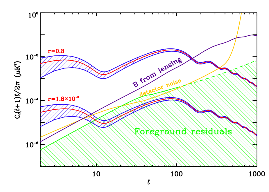
Figure 8: The detectable range of the tensor-to-scalar ratio with a next generation CMB experiment whose frequency band selection is optimized following the calculation presented here. The lower and upper curves for primordial B-modes show an amplitude with a tensor-to-scalar ratio of 0.3 and $1.8\times 10^{-3}$ respectively, roughly indicating the current upper limit on $r$ and the limit reachable with this experiment. The green hatched area is the region where residual foreground noise dominates, due to both polarized dust and synchrotron. The detector noise shows the variance with $\sqrt{2/(2\ell+1)/f_{sky}}N_{\ell}^{\rm noise}$. The curve labeled “B from lensing” is the lensing generated B-mode power spectrum which acts as an additional source of irreducible noise. We assume a survey of 66% of the sky over 2 years.

II.5 Results

We performed the foreground cleaning technique outlined in Section II.3 on the four experiments tabulated in Table 1 and described in Section II.2. We considered both E and B mode power spectrum measurements. Since the main template polarization map from WMAP at 23 GHz has a resolution of about 1 degree, we limited our discussion to angular scale between $\ell=2$ and 100. With higher resolution maps, such as in a few years from Planck, our procedure can be easily extended to account for a wider multipole range. Limiting our discussion to a multipole of about 100 is adequate since the primordial tensor mode power spectrum in CMB B-modes has two significant bumps at $\ell$ of 10, associated with reionization scattering, and at $\ell$ of 100, associated with the horizon size at the matter-radiation equality Pritchard . The ongoing and planned experiments target these two bumps, though ground-based observations are mostly restricted to the bump at $\ell$ of 100 due to large cosmic variance at low multipoles and large scale systematics due to atmospheric emission.

In terms of the experiments outlined in Table 1, experiment C performed worse than the other options as only two frequencies are covered and the foregrounds, on average, dominate over primordial CMB power at the frequencies selected for observations. For experiment C, the main contaminant is the residual dust at 90 GHz (see, figures 4 and 5). Experiment A, while covering a wide range of frequencies, suffers from a low signal-to-noise in each of the channels as the experiment targets a wider area in 10 days. This low signal-to-noise ratio only allows foregrounds to be removed adequately at low multipoles, while at a multipole of 100, detector noise at each of the frequencies starts to dominate and no foreground discrimination is possible. As can be seen from Table 1, experiment D with a wide range of frequency coverage and extremely high sensitivity, easily separates foregrounds over the multipole range of interest. This kind of frequency coverage and high sensitivity is achievable from space.

The discussion, so far, has focused on the ability of each experiment to remove and reduce the foreground contamination. However, there is already a good template for the synchrotron emission on large angular scales at 23 GHz from WMAP. Thus, one can improve the removal further by making use of polarization maps from WMAP. To study this we include WMAP as additional channels. While other multifrequency maps are available, what is important for this analysis is the low-frequency anchor provided by WMAP at 23 GHz. To further improve the sensitivity, we added WMAP data assuming 8 years of observation.

As shown in the middle column of Figs. 4 and 5, while the recovered power spectrum improve for experiments C, the residual foreground level still dominates the $r=0.3$ CMB B-mode power on angular scales of a few degrees owing to the limited B mode polarization reach of WMAP even with 8 years of data. Note that when adding WMAP8 (or Planck below) to experiments A-D, we are only using WMAP8 or Planck to help clean foregrounds and add to the signal in the patch of the sky observed by experiments A-D.

In mid-2008, Planck will be launched and will make CMB polarization measurements over a 14 month period over the whole sky. The polarization maps are expected to have sensitivities roughly a factor of 10 better than 8-year WMAP data Planck06 . Furthermore, Planck will provide anchors at both low- and high-frequency ends tracing both synchrotron and dust, respectively. With 14-month polarization data, and using both the lowest and highest frequency bands as tracers of foreground polarization, we computed the residual foreground level for the same four experiments. We include all the Planck channels (HFI and LFI) in our analysis. The results are summarized in the right column of Figs. 4 and 5. As shown in these figures, Planck data improves foreground removal significantly compared to WMAP. This is because Planck has information at higher frequencies than WMAP, say at 150 GHz and above, where dust polarization dominates with Planck capturing that information out to a frequency of 353 GHz.

An experiment such as C which is limited by residual dust at 90 GHz, when combined with Planck, can limit the tensor-to-scalar ratio to be below 0.02 at the 99% confidence level, as shown by the $r$ estimate. Similarly, a ground-based experiment such as B which is limited by residual synchrotron at low frequencies can be combined with WMAP 8-year data to limit the tensor-to-scalar ratio to be 0.026 at the 99% confidence level. Note that this limit is better than that for the combination of experiment B and Planck which leads to 0.035 at the 99% confidence level. This traces primarily to the fact that while the low noise channels of WMAP 8-year data are effective at removing synchrotron foreground, the high frequency channels of experiment B (though low noise) is not at adequate for an improved removal of synchrotron when combined with Planck. Just as the combination of B and WMAP8 is better, the combination of C and Planck is also better due to differences in the frequency coverage. In general, when we compare experiments A, B or C alone, plus Planck and with Planck alone, there is an improvement of a factor between 2 and 40 in the tensor-to-scalar ratio limit. This shows that ground-based experiments and Planck complement each other, the former by providing a CMB channel with very low noise level, the latter by providing good foreground estimates.

Note that, however, these limits are a factor of 2 to 4 within the published target goal 0.01 of the Inflation Probe Weiss . Our study thus shows that the limit of 0.02 to 0.04 at the 99% confidence may be achieved from the ground with experiments that target an area about or slightly less than 3% of the sky with two to three-year integration to improve sensitivity, and with the help of either WMAP 8-year or Planck data depending on the frequency range of the ground-based experiment. Our study further shows that it is unlikely that any ground-based experiment, when combined with either WMAP8 or Planck, will reach the published goal of 0.01 at the 99% confidence level. The two experiments B and C we have considered are long-term goals of some of the existing experiments. Thus, these capture what is to be expected after Planck is launched and involve significant number of detectors in the focal plane integrating for a long time relative to some of the on going CMB experiments. Thus, it is reasonable for us to state that to reach the published goal of 0.01 within a year of observations, one must consider observations from space.

Experiment	av. noise1	av. noise var.1	av. fgd res.1	$r_{g}$	$r$
A	951.4	196.6	361.7	0.23	0.29
B	18.6	15.3	13.8	0.03	0.05
C	10.3	7.0	558.4	0.39	0.87
D	13.0	4.3	3.2	0.0046	0.0056
A+WMAP8	942.2	190.7	212.1	0.15	0.18
B+WMAP8	18.3	14.6	5.8	0.020	0.026
C+WMAP8	63.8	72.4	345.5	0.36	0.81
D+WMAP8	12.7	4.2	2.8	0.0044	0.0054
A+Planck	389.2	79.0	43.2	0.07	0.10
B+Planck	18.3	14.7	8.3	0.024	0.035
C+Planck	23.2	16.0	2.8	0.018	0.019
D+Planck	12.8	4.2	3.0	0.0045	0.0055
Planck	1803.4	266.3	102.9	0.17	0.19

Table 2: Notes — ¹ values in $10^{-4}\mu$K², see Section II.4 for details. Here, $r_{g}$ & $r$ are the tensor-to-scalar limits reachable by a given experiment assuming repectively that the residuals are an extra Gaussian noise or a fixed foreground. See Section II.4 for details.

III Experimental Optimization To Minimize Foregrounds

In addition to studying the effect of foregrounds on each of these four hypothetical experiments, we also designed an optimized experiment to minimize the foregrounds. The optimization involves the selection of frequency channels such that foregrounds are maximally removed. Throughout this study we assume that the total number of detectors in the focal plane is fixed to be 1000.

For this optimization, we extend the algorithm in Ref. Tegetal03 to allow for a non-uniform weighting of the frequency bands. This is done by introducing a weight vector ${\bf b}$ for the noise such that individual $b^{i}$ coefficients are equal to the inverse of the square root of the number of detector in each channel $i$. Equation 3 gets modified as,

$$\langle|a_{\ell m}|^{2}\rangle={\bf w_{\ell}}^{T}{\cal S}{\bf w_{\ell}}+{\bf w_{\ell}^{\prime}}^{T}{\cal N}{\bf w_{\ell}^{\prime}}\,.$$ (11)

Here, the matrix ${\cal S}$ is the signal (including foregrounds) correlation matrix and ${\cal N}$ is the noise correlation matrix. The coefficients $w^{\prime i}_{\ell}$ are equal to $w^{i}_{\ell}\,b^{i}$. To optimize the frequency channels, we fixed the normalization of the $b^{i}$ coefficient so that $\sum_{i}{(b^{i})^{-2}}=N_{d}$ where $N_{d}$ represents the total number of detectors and numerically solved for the $b^{i}$ coefficient at each frequency. For each $b$ vector, $w^{i}_{\ell}$’s are obtained by following the same procedure as before.

We also include the sky coverage in our optimization study by considering different options for sky coverage assuming total integration time is fixed. In the context of B-mode observations, the optimal sky area required to maximize the sensitivity to primordial tensor modes has been studied in the literature. With foregrounds ignored and the optical depth to reionization assumed to be zero, Ref. KamJaf00 showed that a small patch of a few square degrees may be adequate to detect primordial B-modes as the B-mode spectrum peaks at $\ell$ of 100 associated with the projection of the horizon size at the matter-radiation equality. With the bump at $\ell\sim 10$ included, for models with optical depth to reionization about 0.1 and higher, the optimal sky area becomes larger for CMB polarization experiments that attempt to detect this bump and use it as the primary means to detect tensor modes. Furthermore, if lensing B-modes are the dominant contribution, then almost all-sky data are required for an analysis of lensing confusion Kesden .

However, in all these prior discussions related to sky coverage optimization, contamination from foregrounds was ignored. We emphasize that with polarized foregrounds dominating the E-mode primordial power spectrum at most frequencies and the B-mode power spectrum for $r<0.1$ by a large factor at all frequencies, sky coverage becomes inextricably linked to foreground removal. Instead of treating $f_{\rm sky}$ as a random variable, we consider three specific options here by selecting 3 different sky areas for optimization. These 3 sky coverages are simply areas of the sky where the absolute value of the galactic latitude is higher than 20, 40, 60 degrees, and cover respectively 65.8, 35.7, 13.4% of the entire sky. Note that in each of the three cases, the total integration time is fixed so that the noise in an individual pixel in smaller area maps is lower relative to the pixel noise in a larger area map. We note that the sky cuts we make are not necessarily optimal since the dust and synchrotron emission are not symmetric with respect to the galactic disk as can be seen in Figure 2. We leave this more detailed optimization to a future study.

Freq. (GHz)	30	45	70	100	150	220	340	500
NET/det1	71.7	60.1	50.7	46.0	46.0	60.1	172.5	1310.1
$f_{\rm sky}$
65.8%	31	97	0	163	416	0	215	78
35.7%	26	83	0	10	571	0	230	80
13.4%	30	98	0	0	584	0	212	76

Table 3: Notes — Optimal detector distributions in our 8 frequencies for the different sky coverages assuming the total number of detectors (1000) is fixed. The distributions for the three sky coverages are similar and such that 40-60% of the detectors are assigned to CMB 150 GHz channel, 30-35 % at high frequencies to measure polarized dust, and 10-15 % at low frequencies to measure the polarized synchrotron radiation. ¹The tabulated NET values, per detector, are in $\mu$K$\sqrt{\rm sec}$ and are consistent with values quoted for bolometric observations from space Bock .

	Sky coverage	average noise	average noise variance	average foreground residual	$r_{g}$	$r$	optimization improvement
Lensing	65.8%	1000	150	180	0.0012	0.0014	1.72/1.02
Ignored	35.7%	483	100	131	0.0011	0.0014	1.69/1.27
	13.4%	172	58	41	0.0007	0.0015	1.85/1.78
With	65.8%	1000	150	180	0.0027	0.0018	1.72/1.27
Lensing	35.7%	483	100	131	0.0036	0.0028	1.69/1.23
	13.4%	172	58	41	0.0054	0.0132	1.85/1.09

Table 4: Average (between $\ell=2$ and $100$) level of residual foreground and noise ($C_{\ell}(\ell+1)\ell/2\pi$, units are in nK²) after foreground removal for different sky coverages. The “average noise variance” represents the noise residual once an estimate of the noise power spectrum is subtracted. $r_{g}$ & $r$ are the tensor-to-scalar limits reachable by a given experiment assuming repectively that the residuals are an extra Gaussian noise or a fixed foreground. We quote $r_{g}$ for comparison but stress that it is unlikely that the residuals can be treated as extra Gaussian noise. See Section II.4 for details. The optimization improvement values are the ratio of foreground residual (left) and of $r$ (right) between the non-optimized and optimized setup. The top three lines ignore the additional noise related to lensing B-modes, while the bottom three lines calculate the minimum tensor-to-scalar ratios with lensing B-modes included as a residual noise so that $R_{\ell}=R_{\ell}^{\rm fore}+C_{\ell}^{\rm BB,lens}$. As tabulated, B-mode lensing confusion leads to a factor of 2 to 8 degradation in the minimum tensor-to-scalar ratio suggesting that “lens cleaning” techniques can be implemented to recover this reduction in part.

III.1 Optimization Results

Following the above procedure, we optimized the channel selection for the three sky cuts mentioned above and by making use of the single between $\ell$ of 2 and 100 to detect primordial B-modes. The “optimal” frequency distribution (see, Table 3) is characterized by the dominance of the “CMB channel” (here 150 GHz), which represents 40 to 60% of the total number of detectors, with adequate coverage at both high and low frequencies for removal of dust and synchrotron respectively. Note that this optimization does not include data from other experiments since we have already seen that experiment D, which is our example space-based experiment, shows no improvement when combined with either 8 years of WMAP data or Planck data. As tabulated in Table 3, frequency optimization is such that the number of detectors is higher in the primary CMB channel of 150 GHz than the number of detectors in other channels. In terms of the overall focal plane sensitivity, the fractional contribution from detectors at 150 GHz is even higher since the instrumental noise for detectors at this frequency is the lowest (see second line of Table 3).

As shown in Table 3, our algorithm also selected the two channels at both the lowest and highest frequencies to remove synchrotron and dust, representing respectively about 10 to 13 % and 28 to 32 % of the total number of detectors. This arrangement is necessary to study how the spectrum changes across the sky and the number of detectors is selected in such a way that the resulting noise associated with the uncertainty of the spectral indices of either one of the two foregrounds does not dominate the overall noise. We remind the reader that our spectral indices vary across the sky but they don’t change with frequency. In these foreground channel pairs, the dominant ones are 45 GHz and 340 GHz (in terms of the number of detectors at those channels) because of their raw sensitivity, and the large number of detectors compensates for a smaller arm leverage (see Figure 1). Furthermore, in our optimization almost 50% of the detectors go to the channel at 150 GHz which acts as the primary channel for CMB measurements.

The achievable limits on the tensor-to-scalar ratio are highlighted in Table 4. We tabulated results with and without lensing B-modes as a source of noise. If lensing B-modes could be reduced to a level lower than the residual foreground, the minimum $r$ achievable is 1.4$\times 10^{-3}$ obtained by covering 36% or 66% of the sky. Including lensing as an irreducible noise such that $R_{\ell}=R_{\ell}^{\rm fore}+C_{\ell}^{\rm BB,lens}$ leads to minimum tensor-to-scalar ratios of 1.8$\times 10^{-3}$, 2.8$\times 10^{-3}$, and 1.3$\times 10^{-2}$ for respectively 65.8, 35.7, 13.4 % sky coverage. The 66% sky coverage is more efficient on these very large scales, but the lensing B-modes provide a floor to the primordial B-mode detection there. However on these very large scales, this limit is sensitive to the exact shape of the B-mode reionization bump which in turn depends on the optical depth and the reionization history. In general, our limits show that the suggested $r<0.01$ goal of the next generation Inflation Probe mission (see the report of the Task Force on CMB Research Weiss ) is achievable.

In the last column of Table 4, we highlighted the improvement on the foreground residual and the minimum $r$ when the experiment is optimized relative to an experiment where all the detectors are equally distributed in number between the 8 channels, with 125 detectors per channel. As tabulated, optimization leads to roughly a 70% improvement in the foreground residual and a 2 to 80% improvement in the minimum tensor-to-scalar ratio measurable with each of the three options without lensing contamination. However when the lensing is the limiting factor, the 70% gain on the foreground level only leads to a 9% to a 27% improvement.

As discussed above, in addition to residual foreground noise, with a high sensitivity space-based experiment one must also account for the lensing B-mode signal that acts as another source of confusion Kesden ; Song ; Seljak:2003pn . In Table IV, we also listed the limits on tensor-to-scalar ratio when lensing is ignored so that one can compare the degradation related to lensing alone. As shown by the difference, with lensing included as a source of noise, the resulting constraints on the tensor-to-scalar ratio is a factor of 3 to 6 worse compared to the case when the confusion from lensing B-modes is not present. We highlighted this primarily due to the fact that techniques have been developed to reconstruct the lensing deflection angle and to partly reduce the B-mode lensing confusion when searching for primordial gravitational waves HuOka02 ; Kesden03 ; Hirata03 . These construction techniques make use of the non-Gaussian signal generated in the CMB sky by gravitational lensing. The lensing signal has a unique non-Gaussian pattern captured by a zero three-point correlation function and a non-zero four-point correlation function. This non-Gaussian feature will be very useful for cleaning the lensing signal but detrimental when trying to measure it because of the increased sample variance Smith04 ; Smith06 . However, residual foregrounds are also non-Gaussian and they could bias the extraction of the lensing signal. Thus, in addition to an increase in the power-spectrum noise, foregrounds may also impact proposed techniques to clean the lensing signal. In an upcoming paper, we will discuss the impact of residual foregrounds on these lensing analyses.

IV Conclusions

The B-modes of Cosmic Microwave Background (CMB) polarization may contain a distinct signature of the primordial gravitational wave background that was generated during inflation and the amplitude of the background captures the energy scale of inflation. Unfortunately, the detection of primordial CMB B-mode polarization is significantly confused by the polarized emission from foregrounds, mainly dust and synchrotron within the galaxy. Based on polarized maps from WMAP third-year analysis, which include information on synchrotron radiation at 23 GHz, and a model of the polarized dust emission map, we considered the ability of hypothetical CMB polarization experiments with frequency channels between 20 GHz and 300 GHz to separate primordial CMB from galactic foregrounds. Planck data will aid experiments with narrow frequency coverage to reduce their foreground contamination and we found improvements of factors of 2 to 40 in their achievable $r$.

We also studied an optimization of the distribution of detectors among frequency channels of a CMB experiment with a fixed number of detectors in the focal plane. The optimal configuration (to minimize the amplitude of detectable primordial B-modes) requires observations in at least 5 channels widely spread over the frequency range between 30 GHz and 500 GHz with substantial coverage at frequencies around 150 GHz. If a low-resolution space experiment concentrates on roughly 66% of the sky with the least contamination, and with 1000 detectors reach a noise level of about 1000 (nK)², the minimum detectable level of the tensor-to-scalar ratio would be about 0.002 at the 99% confidence level. The bulk of the sensitivity comes from the largest angular scales, i.e., using the signal created during reionization.

Our results indicate that the goal for the next generation Inflation Probe mission as outlined in the recent report from the Task Force on CMB Research Weiss is achievable.

Acknowledgments: We would like to acknowledge the use of the HEALPix package for our map pixelization Gorski and participants of the Irvine Conference on “Fundamental Physics with CMB Radiation” for useful discussions and suggestions that led to this work. We thank the WMAP flight team and NASA office of Space Sciences for making available processed WMAP data public from the Legacy Archive for Microwave Background Data Analysis (LAMBDA). This work is supported by a McCue Fellowship to AA at UC Irvine Center for Cosmology.

References

- (1) W. Hu, N. Sugiyama and J. Silk, Nature 386, 37 (1997) [arXiv:astro-ph/9604166].
- (2) P. J. E. Peebles and J. T. Yu, Astrophys. J. 162, 815 (1970).
- (3) R. A. Sunyaev and Y. B. Zeldovich, Astrophys. Space Sci. 7, 3 (1970).
- (4) R. K. Sachs and A. M. Wolfe, Astrophys. J. 147, 73 (1967).
- (5) J. Silk, Astrophys. J. 151, 459 (1968).
- (6) G. Hinshaw et al., arXiv:astro-ph/0603451.
- (7) D. N. Spergel et al., arXiv:astro-ph/0603449.
- (8) W. Hu and S. Dodelson, Ann. Rev. Astron. Astrophys. 40, 171 (2002) [arXiv:astro-ph/0110414].
- (9) M. Zaldarriaga, Phys. Rev. D 55, 1822 (1997) [arXiv:astro-ph/9608050].
- (10) L. Page et al., arXiv:astro-ph/0603450.
- (11) A. A. Starobinsky, JETP Lett.30, 682 (1979)
- (12) M. Kamionkowski and A. Kosowsky, Ann. Rev. Nucl. Part. Sci. 49, 77 (1999) [arXiv:astro-ph/9904108].
- (13) M. Kamionkowski, A. Kosowsky and A. Stebbins, Phys. Rev. D 55, 7368 (1997) [arXiv:astro-ph/9611125].
- (14) U. Seljak and M. Zaldarriaga, Phys. Rev. Lett. 78, 2054 (1997) [arXiv:astro-ph/9609169].
- (15) L. Verde, H. Peiris and J. Raul, JCAP, 1, 19 (2006) [arXiv:astro-ph/0506036].
- (16) M. Amarie, C. Hirata and U. Seljak, Phys. Rev. D 72, 123006 (2005) [arXiv:astro-ph/0508293].
- (17) E. Carretti, G. Bernardi and S. Cortiglioni, arXiv:astro-ph/0609288.
- (18) M. Kesden, A. Cooray and M. Kamionkowski, “Separation of gravitational-wave and cosmic-shear contributions to cosmic Phys. Rev. Lett. 89, 011304 (2002) [arXiv:astro-ph/0202434].
- (19) L. Knox and Y. S. Song, Phys. Rev. Lett. 89, 011303 (2002) [arXiv:astro-ph/0202286].
- (20) U. Seljak and C. M. Hirata, “Gravitational lensing as a contaminant of the gravity wave signal in Phys. Rev. D 69, 043005 (2004) [arXiv:astro-ph/0310163].
- (21) M. Kaplinghat, L. Knox and Y. S. Song, Phys. Rev. Lett. 91, 241301 (2003) [arXiv:astro-ph/0303344].
- (22) D. J. Schlegel, D. P. Finkbeiner and M. Davis, Astrophys. J. 500, 525 (1998) [arXiv:astro-ph/9710327].
- (23) J. L. Jonas, E. E. Baart and G. D. Nicolson, Mon. Not. R. Astron. Soc. 297, 977 (1998).
- (24) W. Reich, Astron. Astrophys. 48, 219 (1982).
- (25) P. Reich and W. Reich, Astron. Astrophys. 63, 205 (1986).
- (26) C. G. T. Haslam, H. Stoffel, S. Kearsey, J. L. Osborne and S. Phillips, Nature 289, 470 (1981).
- (27) N. Ponthieu et al., “Temperature and polarization angular power spectra of Galactic dust Astron. Astrophys. 444, 327 (2005) [arXiv:astro-ph/0501427].
- (28) P. G. Martin, “On Predicting the Polarization of Low Frequency Emission by Diffuse arXiv:astro-ph/0606430.
- (29) The Planck Collaboration, “The Scientific Programme of Planck” arXiv:astro-ph/0604069.
- (30) D. P. Finkbeiner, M. Davis and D. J. Schlegel, “Extrapolation of Galactic Dust Emission at 100 Microns to CMBR Frequencies Astrophys. J. 524, 867 (1999) [arXiv:astro-ph/9905128].
- (31) A. Lazarian and B. T. Draine, Astrophys. J. 536, L15 (2000).
- (32) T. E. Montroy et al., Astrophys. J. 647, 813 (2006) [arXiv:astro-ph/0507514].
- (33) W. Hu, M. M. Hedman and M. Zaldarriaga, Phys. Rev. D 67, 043004 (2003) [arXiv:astro-ph/0210096].
- (34) E. F. Bunn, Phys. Rev. D 65, 043003 (2002) [arXiv:astro-ph/0108209].
- (35) K. M. Smith, arXiv:astro-ph/0511629.
- (36) M. Tegmark, A. de Oliveira-Costa and A. Hamilton, Phys. Rev. D 68, 123523 (2003) [arXiv:astro-ph/0302496].
- (37) M. Kaplinghat, M. Chu, Z. Haiman, G. Holder, L. Knox and C. Skordis, Astrophys. J. 583, 24 (2003) [arXiv:astro-ph/0207591].
- (38) A. H. Jaffe, M. Kamionkowski and L. M. Wang, Phys. Rev. D 61, 083501 (2000) [arXiv:astro-ph/9909281].
- (39) J. R. Pritchard and M. Kamionkowski, Annals Phys. 318, 2 (2005) [arXiv:astro-ph/0412581].
- (40) J. Bock et al., arXiv:astro-ph/0604101.
- (41) J. Bock, private communication (2006).
- (42) W. Hu and T. Okamoto, Astrophys. J. 574, 566 (2002) [arXiv:astro-ph/0111606].
- (43) M. H. Kesden, A. Cooray and M. Kamionkowski, Phys. Rev. D 67, 123507 (2003) [arXiv:astro-ph/0302536]; A. Cooray and M. Kesden, New Astron. 8, 231 (2003) [arXiv:astro-ph/0204068].
- (44) C. M. Hirata and U. Seljak, “Reconstruction of lensing from the cosmic microwave background Phys. Rev. D 68, 083002 (2003) [arXiv:astro-ph/0306354].
- (45) K. M. Gorski, E. Hivon, A. J. Banday, B. D. Wandelt, F. K. Hansen, M. Reinecke and M. Bartelman, “HEALPix – a Framework for High Resolution Discretization, and Fast Astrophys. J. 622, 759 (2005) [arXiv:astro-ph/0409513].
- (46) K. M. Smith, W. Hu and M. Kaplinghat, Phys. Rev. D 70, 043002 (2004) [arXiv:astro-ph/0402442].
- (47) K. M. Smith, W. Hu and M. Kaplinghat, arXiv:astro-ph/0607315.