Intermediate inflation in light of the three-year WMAP observations

Abstract

The three-year observations from the Wilkinson Microwave Anisotropy Probe have been hailed as giving the first clear indication of a spectral index $n_{\mathrm{s}}<1$. We point out that the data are equally well explained by retaining the assumption $n_{\mathrm{s}}=1$ and allowing the tensor-to-scalar ratio $r$ to be non-zero. The combination $n_{\mathrm{s}}=1$ and $r>0$ is given (within the slow-roll approximation) by a version of the intermediate inflation model with expansion rate $H(t)\propto\ t^{-1/3}$. We assess the status of this model in light of the WMAP3 data.

I Introduction

The most striking result from the three-year Wilkinson Microwave Anisotropy Probe (WMAP) observations wmap3 is the pressure that they impose on the Harrison–Zel’dovich spectrum of density perturbations, for which adiabatic perturbations have the scale-invariant spectral index $n_{\mathrm{s}}=1$. This spectrum was first proposed by Harrison harr and Zel’dovich zeld because it has metric potential perturbations of the same amplitude on all scales. This allows small perturbation theory to hold on large and small scales, and would also allow primordial black-hole formation to occur over a wide range of mass scales if the amplitude of fluctuations was sufficiently large CH . Harrison–Zel’dovich spectra arise in pure de Sitter inflationary universe models, but they  have also been shown to arise from different non-inflationary cosmological situations branpeter .

The simplest versions of inflation, in which a finite period of de Sitter-like inflationary expansion occurs, naturally create such a spectrum of fluctuations because the dynamics have no preferred moment of time in de Sitter spacetime: an irregularity spectrum with identical metric perturbations on each scale respects this invariance. However, there are many variants of inflation for which the expansion dynamics are not of de Sitter form, and they predict different spectra of fluctuations; hence it is important to determine which (if any) of them are consistent with the current observational data. If adiabatic density perturbations are the only perturbations present, then the original WMAP3 parameter-estimation analysis suggested that the Harrison–Zel’dovich spectrum is excluded at quite high significance wmap3 . This significance has been reduced by re-analysis of the inflationary constraints by the WMAP team (available at Ref. wmapanal ), from the viewpoint of the more sophisticated statistical approach of model selection PML , and by recent papers highlighting possible systematic effects syspapers , but it is nevertheless timely to explore possible interpretations of these data.

The conclusion that $n_{\mathrm{s}}=1$ is disfavoured by the data is restricted to the case where adiabatic scalar perturbations are the only ones present. The best-motivated generalization is the inclusion of tensor perturbations, which are predicted to be present at some level by inflation, and parametrized by the tensor-to-scalar ratio $r$. This is explored in some detail by the WMAP team wmap3 , and in subsequent papers nrcons , with the conclusion that $n_{\mathrm{s}}\geq 1$ is readily allowed provided that the value of $r$ is significantly non-zero.

In this Brief Report, we analyze a particular class of inflationary models which give this behaviour, the intermediate inflation model discussed in Refs. inter ; mus ; rendall . This was originally introduced as an exact inflationary solution for a particular scalar field potential, but is perhaps best-motivated as the slow-roll solution to potentials which are asymptotically of inverse power-law type, $V\propto\phi^{-\beta}$. This type of potential is in common use in quintessence models RPmodel , but it also gives viable inflationary solutions, although with this precise potential form inflation is everlasting and a mechanism has to be introduced to bring inflation to an end. It also arises in a range of scalar–tensor gravity theories maeda .

As shown by Barrow and Liddle BL , the intermediate inflationary model, in the slow-roll approximation, gives $n_{\mathrm{s}}=1$ to first order provided $\beta=2$ (see also Ref. valli for a more extensive discussion of the inflationary generation of the Harrison–Zel’dovich spectrum, and Ref. starob for the construction of exact potentials giving $n_{{\rm S}}=1$ without slow-roll approximation). In this case, $r$ depends significantly on scale, falling in value with time and hence becoming smaller on shorter length-scales. There will be an observable effect provided inflation ends swiftly enough, so that $r$ was still important at the horizon crossing of observable perturbations. More generally, if $\beta\neq 2,$ the spectral index may exhibit running, approaching unity at late times; see also the review of this situation in Ref. nrcons .

II Predictions of the model

A generalization of the intermediate inflation model inter used in the earlier study of Ref. BL has an expansion scale factor given by (with appropriate choice of time coordinate)

$$a(t)=\exp\left(At^{f}+Bt\right)\,,$$ (1)

$$\qquad\quad 0<f<1,\quad A>0,~{}B\geq 0,\;\mathrm{constants}\,.$$

This is an exact solution of the Friedmann equations ($8\pi G=c=\hbar=1$) for a flat universe containing a scalar field $\phi(t)$ with potential $V(\phi)$, where

$$\phi = \phi_{0}+\left[\frac{8A(1-f)}{f}\right]^{1/2}\;t^{f/2}\,,$$ (2)

$$V(\phi) = 3\left\{B+Af\left[\frac{f}{8A(1-f)}\right]^{(f-1)/f}(\phi-\phi_{0})^{2(f-1)/f}\right\}^{2}-Af(1-f)\left[\frac{f}{8A(1-f)}\right]^{(f-2)/f}(\phi-\phi_{0})^{2(f-2)/f}\,.\;\;$$ (3)

It can be obtained using the solution-generating method of Ref. pb . Without loss of generality $\phi_{0}$ can be taken to be zero. We will now specialise to the pure intermediate inflationary model of Refs. inter ; BL with $B=0$ and $A>0$.

In the slow-roll approximation with $B=0$, the first term on the RHS of Eq. (3) dominates $V$ at large $\phi$, and we have

$$\phi = (2A\beta t^{f})^{1/2}\quad\mathrm{where}\;\;\beta\equiv 4(f^{-1}-1)\,;$$ (4)

$$V(\phi) = \frac{48A^{2}}{(\beta+4)^{2}}(2A\beta)^{\beta/2}\phi^{-\beta}\,,$$ (5)

as the scalar field rolls down a power-law potential. The first two slow-roll parameters are then given, in the Hamilton–Jacobi formalism LPB , by

$$\epsilon=\frac{\beta^{2}}{2\phi^{2}},\quad\eta=\beta\left(1+\frac{\beta}{2}\right)\frac{1}{\phi^{2}}\,.$$ (6)

So, the condition for inflation to occur ($\epsilon<1$) is only satisfied when $\phi^{2}>\beta^{2}/2$.

II.1 First-order considerations

In order to confront this model with observations, we need to consider the contribution of the scalar and tensor perturbations which can be represented by $n_{\mathrm{s}}$ and $r$, respectively. They are expressed in terms of the slow-roll parameters to first order by LL

$$n_{\mathrm{s}} = 1-4\epsilon+2\eta=1-\frac{\beta(\beta-2)}{\phi^{2}}$$ (7)

$$r = 16\epsilon=\frac{8\beta^{2}}{\phi^{2}}$$ (8)

We clearly see that $n_{\mathrm{s}}=1$ and $r>0$ is possible, provided $\beta=2$. This is the case where $\eta=2\varepsilon$. We see that an exact scale-invariant spectrum can be obtained to leading order in slow-roll by both the de Sitter expansion, i.e. with $a(t)=\exp(H_{0}t)$ and $H_{0}$ constant, and by the special intermediate inflationary dynamics with $a(t)=\exp(At^{2/3})$.

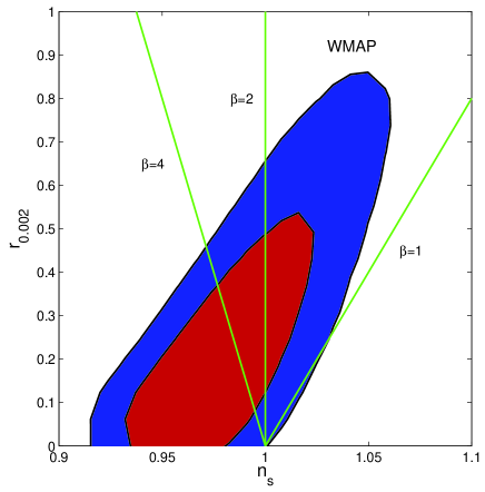
Figure 1: Trajectories for different values of the parameter $\beta$ in the $n_{\mathrm{s}}$–$r$ plane, to first-order in slow roll. From left to right $\beta=4$, 2, 1. The two contours correspond to the 68% and 95% levels of confidence. The observational data is from the WMAP analysis at Ref. wmapanal , which updates that of version 1 of Ref. wmap3 . The observational dataset used is WMAP alone, applied to the lcdm+tens model (without spectral index running).

Returning to the general case ($0<f<1$), this model can be compared with observations, shown in Fig. 1. The relation between the scalar and tensor perturbations is

$$n_{\mathrm{s}}=1-\frac{\beta-2}{8\beta}r.$$ (9)

On one hand, we see that $\beta>2$ is well supported by the data, while on the other, we see that $\beta<2$ allows $n_{\mathrm{s}}>1$, but becomes rapidly disfavoured when $\beta$ approaches $1$.

In order for our comparison of the intermediate inflationary model’s predictions with the observations to be complete, we must also consider the time spent by the field in the region of the $n_{\mathrm{s}}$–$r$ plane allowed by the data. The number of $e$-foldings between two different values $\phi_{1}$ and $\phi_{2}$ of the scalar field is given by BL

$$N(\phi_{1},\phi_{2})=\frac{1}{2\beta}(\phi_{2}^{2}-\phi_{1}^{2})\,.$$ (10)

If we assume that inflation begins at the earliest possible stage, that is at $\phi_{1}^{2}=\beta^{2}/2$, then Eqs. (7) and (8) can be re-expressed in terms of the number of $e$-foldings, $N_{b}$, which have passed since the beginning of the inflationary period:

$$n_{\mathrm{s}} = 1-\frac{2\beta-4}{4N_{b}+\beta},$$ (11)

$$r = \frac{16\beta}{4N_{b}+\beta}.$$ (12)

If we consider a Harrison–Zel’dovich model ($\beta=2$) with the inclusion of gravitational waves, then we see in Fig. 1 that the curve $r=r(n_{\mathrm{s}})$ enters the 95% confidence region for $r=0.66$ which corresponds to $N_{b}\simeq 12$. Since the point $(n_{\mathrm{s}}=1$, $r=0)$ lies just inside the two-dimensional 95% confidence contour, the model is viable for all larger values of $N_{b}$.

II.2 Second-order corrections

Next, we show that the second-order corrections to our analysis at first-order in slow roll are small, and can be neglected to a very good approximation. Generalizing Eq. (7) in terms of the slow-roll parameters to second-order, we have LL ; SL

$$n_{\mathrm{s}}-1=2\eta-4\epsilon-[8(1+C)\epsilon^{2}-(6+10C)\epsilon\eta+2C\xi^{2}],$$ (13)

with $C=-0.73$ a known numerical constant, and $\xi^{2}(\phi)\equiv\epsilon\eta-(2\epsilon)^{1/2}\,d\eta/d\phi$. Putting $\beta=2$ (so that we have $n_{\mathrm{s}}=1$ exactly to first order) in the above expression, we get the second-order correction to the spectral index:

$$n_{\mathrm{s}}-1=4\epsilon^{2}.$$ (14)

Finally, knowing that $r=16\epsilon+O(\epsilon^{2})$, we obtain to second order that

$$n_{\mathrm{s}}-1=\frac{r^{2}}{64}.$$ (15)

The above calculation, which uses the exact solution, corresponds to the full potential Eq. (3). While in the full slow-roll approximation this gives the same result as the single power-law model, Eq. (5), at second-order the potentials yield different results. A similar calculation to the above, but using the $V$-slow-roll approximation LPB , shows that the denominator 64 is modified to $384/7$ in that case.

Observations wmap3 constrain $r$ to be less than $0.65$ (at 95% confidence). So, for either potential, this extra contribution in the case with $\beta=2$ is quite negligible once the field enters the region allowed by the data.

II.3 The running of the spectral index

The running of the spectral index in inflationary models is given, to lowest order in slow-roll, by LL

$$\frac{dn_{\mathrm{s}}}{d\ln k}=-8\epsilon^{2}+10\epsilon\eta-2\xi^{2}=\frac{2\beta^{2}(\beta-2)}{\phi^{4}}.$$ (16)

Moreover, to lowest order $n_{\mathrm{s}}-1=-\beta(\beta-2)\phi^{-2}$, which allows us to rewrite this relation as

$$\frac{dn_{\mathrm{s}}}{d\ln k}=\frac{2}{\beta-2}(n_{\mathrm{s}}-1)^{2}.$$ (17)

We can deduce from this relation that $\beta=2$ implies no running of the spectral index to first-order, which was already obvious from the comment following Eq. (7).

Models with $\beta>2$ feature positive running, which the WMAP3 data disfavor wmap3 ; wmapanal . However, within the allowed region the predicted running is very small (for example, it is always less than 0.001 for the $\beta=4$ case), and it would be premature to claim that the running constraint adds any value to the $n_{\mathrm{s}}$–$r$ constraints for these models.

III Conclusions

The intermediate inflation model is a viable example of a model with $n_{\mathrm{s}}=1$ which is permitted by the observational data, due to the non-zero tensor contribution. In this model, $r$ is scale-dependent, and we have shown that a good fit to the WMAP3 observations is possible provided observable scales crossed outside the horizon at least 12 $e$-foldings after the earliest possible starting-point for inflation. Arranging this requires that whatever mechanism is introduced to bring inflation to an end does so with $\phi>14$ in reduced Planck units, considering that a minimum of perhaps 50 $e$-foldings is required to push the perturbations to observable scales LL .

This model serves as a useful phenomenological illustration, in the light of WMAP3 data, of a type of simple slowly-rolling scalar field evolution that does not display pure de Sitter inflationary expansion, but can still produce a Harrison–Zel’dovich spectrum.

For the more general intermediate inflation case with $\beta\neq 2$, observations constrain $\beta$ to be greater than about one, unless we are in the regime very close to the Harrison–Zel’dovich limit. Constraints from running do not presently add extra information.

References

- (1) D. N. Spergel et al. (WMAP Collaboration), astro-ph/0603449.
- (2) E.R. Harrison, Phys. Rev. D1, 2726 (1970).
- (3) Ya.B. Zel’dovich, Mon. Not. Roy. Astron. Soc. 160, 1P (1972).
- (4) B. Carr and S.W. Hawking, Mon. Not. Roy. Astron. Soc. 168, 399 (1974).
- (5) R.H. Brandenberger, A. Nayeri, S.P. Patil, and C. Vafa, hep-th/0608121; P. Peter, E. J. C. Pinho, and N. Pinto-Neto, hep-th/0610205.
- (6) Legacy Archive for Microwave Background Data Analysis: lambda.gsfc.nasa.gov.
- (7) D. Parkinson, P. Mukherjee, and A. R. Liddle, Phys. Rev. D73, 123523 (2006), astro-ph/0605003.
- (8) H. Peiris and R. Easther, JCAP 0607, 002 (2006), astro-ph/0603587; A. Lewis, astro-ph/0603753; M. Viel, M. G. Haehnelt, and A. Lewis, Mon. Not. Roy. Astron. Soc. 370, L51 (2006), astro-ph/0604310; U. Seljak, A. Slosar, and P. McDonald, astro-ph/0604335; H. K. Eriksen et al., astro-ph/0606088; K. M. Huffenberger, H. K. Eriksen, and F. K. Hansen, astro-ph/0606538.
- (9) W.H. Kinney, E.W. Kolb, A. Melchiorri, and A. Riotto, Phys. Rev. D74, 023502 (2006), astro-ph/0605338; J. Martin and C. Ringeval, JCAP 0608, 009 (2006), astro-ph/0605367; F. Finelli, M. Rianna, and N. Mandolesi, JCAP 0612, 006 (2006), astro-ph/0608277.
- (10) J.D. Barrow, Phys. Lett. B235, 40 (1990); J.D. Barrow and P. Saich, Phys. Lett. B249, 406 (1990).
- (11) A.G. Muslimov, Class. Quantum Grav. 7, 231 (1990).
- (12) A.D. Rendall, Class. Quantum Grav. 22, 1655 (2005), gr-qc/0501072.
- (13) B. Ratra and P. J. E. Peebles, Phys. Rev. D37, 3406 (1988); I. Zlatev, L. Wang, and P. J. Steinhardt, Phys. Rev. Lett. 82, 896 (1999), astro-ph/9807002; A. R. Liddle and R. J. Scherrer, Phys. Rev. D59, 023509 (1999), astro-ph/9809272.
- (14) J.D. Barrow and K.I. Maeda, Nucl. Phys. B341, 294 (1990).
- (15) J.D. Barrow and A.R. Liddle, Phys. Rev. D47, R5219 (1993), astro-ph/9303011.
- (16) A. Vallinotto, E.J. Copeland, E.W. Kolb, A.R. Liddle, and D.A. Steer, Phys. Rev. D69, 103519 (2004), astro-ph/0311005.
- (17) A. A. Starobinsky, JETP Lett. 82, 169 (2005), astro-ph/0507193.
- (18) P. Parsons and J.D. Barrow, Class. Quantum Grav. 12, 1715 (1995).
- (19) A.R. Liddle, P. Parsons, and J.D. Barrow, Phys. Rev. D50, 7222 (1994), astro-ph/9408015.
- (20) A.R. Liddle and D.H. Lyth, Cosmological Inflation and Large-Scale Structure, CUP, Cambridge, 2000; J.E. Lidsey, A.R. Liddle, E.W. Kolb, E.J. Copeland, T. Barreiro, and M. Abney, Rev. Mod. Phys. 69, 373 (1997), astro-ph/9508078.
- (21) E.D. Stewart and D.H. Lyth, Phys. Lett. B302, 171 (1993), gr-qc/9302019.