The morgana model for the rise of galaxies and active nuclei

Abstract

We present the MOdel for the Rise of GAlaxies aNd Active nuclei (morgana), a new code for the formation and evolution of galaxies and AGNs. Starting from the merger trees of dark matter halos and a model for the evolution of substructure within the halos, the complex physics of baryons is modeled with a set of state-of-the-art models that describe the mass, metal and energy flows between the various components (baryonic halo, bulge, disc) and phases (cold and hot gas, stars) of a galaxy. These flows are then numerically integrated to produce predictions for the evolution of galaxies. The processes of shock-heating and cooling, star formation, feedback, galactic winds and super-winds, accretion onto BHs and AGN feedback are described by new models. In particular, the evolution of the halo gas explicitly follows the thermal and kinetic energies of the hot and cold phases, while star formation and feedback follow the results of the multi-phase model by Monaco (2004a). The increased level of sophistication of these models allows to move from a phenomenological description of gas physics, based on simple scalings with the depth of the DM halo potential, toward a fully physically motivated one. We deem that this is fully justified by the level of maturity and rough convergence reached by the latest versions of numerical and semi-analytic models of galaxy formation. The comparison of the predictions of morgana with a basic set of galactic data reveals from the one hand an overall rough agreement, and from the other hand highlights a number of well- or less-known problems: (i) producing the cutoff of the luminosity function requires to force the quenching of the late cooling flows by AGN feedback, (ii) the normalization of the Tully-Fisher relation of local spirals cannot be recovered unless the dark matter halos are assumed to have a very low concentration, (iii) the mass function of HI gas is not easily fitted at small masses, unless a similarly low concentration is assumed, (iv) there is an excess of small elliptical galaxies at $z=0$. These discrepancies, more than the points of agreement with data, give important clues on the missing ingredients of galaxy formation.

1 Introduction

Several datasets spanning a large range of distances and luminosities in most of our past-light cone are now constraining the background cosmology and the properties of primordial fluctuations with a remarkable precision. Temperature fluctuations of the CMB (Spergel et al. 2003, 2006), distant Supernovae (SN, Perlmutter et al, 1999; Knop et al., 2003), the large-scale structure traced by galaxies (2dF, Percival et al. 2002; SDSS, Eisenstein et al. 2005), the statistics of microlensing (Refregier 2003), the abundance and clustering of galaxy clusters (Rosati, Borgani & Norman 2002) and the statistics of the Lyman$\alpha$ forest transmission (Viel, Haehnelt & Springel 2004) are now giving a consistent picture of our Universe, well described by the $\Lambda$CDM model with parameters $(\Omega_{0},\Omega_{\Lambda},\Omega_{b},h,\sigma_{8})\simeq(0.3,0.7,0.04,0.7,0.8)$ (with the last quantity ranging from 0.75 to 09).

This “concordance” model provides the initial conditions for the evolution of perturbations, responsible for the gathering of dark matter (DM) into bound and relaxed halos. These DM halos host most of the astro-physical processes that rule the formation of stars and galaxies from the primordial gas. However, while the initial conditions are specified and the basic physical laws are known, the formation of galaxies is still an open problem, due to the high level of non-linearity of the processes involved and to the wide coupling of scales, from the km scale of imploding cores of SNe to the Mpc scale of galaxy super-winds. Galaxy formation is thus a problem of complexity.

Numerical simulations aimed at resolving galaxies (see, e.g., Pearce et al. 2001; Weinberg, Hernquist & Katz 2002; Steinmetz & Navarro 2002; Mathis et al. 2002; Lia, Portinari & Carraro 2002; Recchi et al. 2002; Toft et al. 2002; Springel & Hernquist 2003; Tornatore et al. 2003; Governato et al. 2004) are still struggling both to tame the full complexity of the problem and to reach a sufficient mass and spatial resolution to resolve the “microphysics” of the injection of energy by SNe and accreting BHs. As a matter of fact, most simulations of single galaxies are limited to mass resolutions of $\sim 10^{5}$ M_⊙ and space resolutions of $\sim 1$ kpc, so the microphysical level is still treated as “sub-grid physics” and inserted in the codes with the aid of simple effective models. The problem is even more severe when trying to introduce accreting BHs within a galaxy (Di Matteo et al. 2003; Kazantzidis et al. 2005), something that many authors regard as the missing ingredient of galaxy formation. Considering then that most constraints on galaxies and AGNs are of a statistical nature, so that thousands if not hundreds of thousands of galaxies need to be produced for each model, it is clear that, at variance with what has happened with DM, a straighforward solution of the galaxy formation problem with N-body simulations is beyond hope for years to come.

A quicker approach is given by the so-called “semi-analytic” galaxy formation models (White & Frenk 1991; Kauffmann et al. 1999; Somerville & Primack 1999; Cole et al. 2000; Wu, Fabian & Nulsen 2000; Granato et al. 2001; Hatton et al. 2003; Menci et al. 2004; Kang et al. 2005; Nagashima et al. 2005; Cattaneo et al. 2006; De Lucia et al. 2006; Bower et al. 2006), where all the processes that take place in the formation of galaxies are taken into account with simple approximated recipes. The main advantage of these models resides in the possibility of predicting the properties of whole galaxy populations in a short amount of computing time, thus making it possible to achieve a good sampling of the parameter space. However, it has been remarked that the (mostly phenomenological) recipes used in these models have often a weak physical motivation and require the inclusion of free parameters that are difficult to constrain otherwise. As a consequence, the agreement between model and data, when achieved, may not shed much light on the process of galaxy formation. Moreover, given the intrinsic complexity of the problem, the models have often struggled to reproduce longly known pieces of evidence, like the shape of the luminosity function of galaxies, without convincingly showing their predictive power. This is highlighted by the difficulties of specific versions of semi-analytic models to reproduce some pieces of evidence, like the high-mass cutoff of the luminosity function (Benson et al. 2003), the normalization of the Tully-Fisher relation (Kauffmann et al. 1999), the sub-mm counts (Baugh et al. 2005), the level of $\alpha$-enhancement in ellipticals (Thomas et al. 2005; Nagashima et al. 2005), the redshift distribution of K-band sources (Cimatti et al. 2002). From this point of view, it is incorrect to claim that these models have too many free parameters, as it is clearly possible to falsify them.

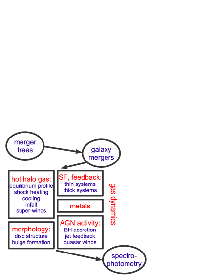
Figure 1: Outline of the main ingredients in the morgana code. Merger trees are taken from the pinocchio tool (Monaco et al. 2002a); galaxy mergers are treated following Taffoni et al. (2003); spectrophotometry is performed with grasil (Silva et al. 1998). The treatment of gas dynamics of baryons within the DM halos is the main argument of the present paper.

This paper is the first of a series devoted to presenting morgana, a new galaxy formation model which, in comparison to the ones listed above, treats many of the physical processes at an increased level of sophistication. Figure 1 shows a general outline of this model, that could be applied to most similar models. The most relevant features of morgana are the following:

• the evolution of the various components and phases of a galaxy is followed by integrating a differential system of equations along each branch of a merger tree, thus allowing for the most general (and non-linear) set of equations for mass, energy and metal flows;

• the halo gas is treated as a multi-phase medium (hot gas, cooling flow, halo stars) and its evolution is described by a model that takes into account the thermal and kinetic energies of the hot and cold phases; this model treats cooling and infall as separated processes, takes into account the mass and energy injection from the galaxy to the halo (galactic winds) and from the halo to the Inter-Galactic Medium (IGM; galactic super-winds);

• feedback and star formation are inserted following the results of the multi-phase model by Monaco (2004a, hereafter M04; 2004b), plus an additional prescription for kinetic feedback;

• accretion onto BHs and its feedback onto the galaxy (through radio jets and quasar-triggered galaxy winds) are built-in.

The increased level of sophistication allows to move from a phenomenological description of gas physics, based on simple scalings with the depth of the DM halo potential, toward a fully physically motivated one.

morgana has not been developed to construct a “theory of everything” for galaxies; we consider this model simply as a precious tool (i) to understand the interplay and relative importance of the various physical processes that take place in galaxy formation, (ii) to incorporate easily more processes that are thought to influence galaxies, so as to test their effects, (iii) to produce mock galaxy catalogues which reproduce particular selection criteria, in order to investigate the properties of galaxy surveys like sample variance and completeness level. The ultimate aim is to increase the predictive power of such galaxy formation models.

On the other hand, the increase in the level of sophistication can only lead to an increase in the number of parameters of the model. Many of these parameters are fixed either by observations (like the cosmological parameters) or purely gravitational N-body simulations (like the parameters related to galaxy mergings), while others can be fixed in principle with the aid of hydro simulations (like the parameters related to gas cooling and super-winds). Besides, fundamental quantities like the energy of a single SN, the Initial Mass Function (IMF) of stars, the chemical yields or the parameters connected to the feedback and accretion onto BHs are very uncertain. This is again a problem of complexity, which will not be solved by neglecting important degrees of freedom. So, instead of decreasing the number of parameters we aim to test our model versus a large number of observational constraints, so as to fix all the parameters and propose predictions for upcoming and future observational campaigns.

This paper presents the algorithm in full detail and some results that show the main potentialities, merits and problems of the model. The stellar mass function produced by this model has already been presented in Fontana et al. (2006). Other upcoming papers will address specific cosmogonical topics, like the statistics of the AGN/quasar population (Fontanot et al. 2006a), the assembly of the stellar mass of bright galaxies (Fontanot et al. 2006b) and the construction of the Stellar Diffuse Component in galaxy clusters (Monaco et al. 2006). The paper is organized as follows: Section 2 presents an outline of the model, describing its structure and the mass, energy and metal flows. The next sections, from 3 to 11, describe in detail the treatment of all the physical processes inserted in the model; the reader willing to skip the details may go directly to section 12. Section 3 describes the merger trees of DM halos, section 4 the merging of galaxies, section 5 the physics of the halo gas phases, section 6 the formation of bulges and discs, section 7 the modeling of stellar feedback, section 8 the production of metals, section 9 the accretion onto BHs. Section 10 discusses the parameters involved in the model, while section 11 outlines the main post-processing phases. Section 12 gives some basic results of the model and compares them to available observations, while section 13 gives the conclusions. Two appendices report details on the merging and destruction times of satellites and a very preliminary analysis of stability with mass resolution.

In this paper we use a “concordance” $\Lambda$CDM cosmology with parameters $\Omega_{0}=0.3$, $\Omega_{\Lambda}=0.7$, $\Omega_{b}=0.044$, $\sigma_{8}=0.9$, $H_{0}=70$ km s^-1 Mpc^-1. All physical quantities are scaled to this $H_{0}$ value. The new WMAP results (Spergel et al. 2006), published when this paper was at a very advanced state of preparation, suggest $\sigma_{8}\simeq 0.75$, and this could lead to some modest though significant changes in the predictions given in this paper.

2 Outline of the model

In this section we outline the model, describing the structure of the code and the system of equations for the mass, energy and metal flows that is integrated by the code.

2.1 DM halos and galaxies

The merger trees of DM halos are obtained using the pinocchio code (the details are given later in section 3.1). This is not considered as an integrated part of the galaxy formation code; any other code for generating merger trees can be used in its place. With respect to the Millennium Simulation (Springel et al. 2005), the pinocchio trees do not give any information on the substructure of DM halos.

Like N-body simulations, pinocchio is based on realizations of Gaussian initial conditions on a cosmological grid, so the mass resolution of merger trees is determined by the grid particle mass. Each DM halo that gets as massive as at least ten particles constitutes a starting branch of the tree; the time at which this happens is named appearance time. A galaxy is associated to each starting branch. When a DM halo merges with a larger one, it disappears as an individual entity and becomes a substructure (or satellite) of the larger DM halo. The fate of substructures is followed using the model of Taffoni et al. (2003; section 4.1): while the external regions of the satellite DM halo are tidally stripped, its core, which contains its associated galaxy, survives for some time. A galaxy that is associated with an existent DM halo is named central; in general (though not always) the central galaxy is the largest in a DM halo. Galaxies associated with substructures are named satellites. Dynamical friction brings the orbit of the substructure toward the centre, making it eventually merge with the main DM halo; when this happens the satellite galaxy merges with the central one. In some cases, the substructure and its associated galaxy can be destroyed by tides. Substructures can also merge between themselves, but this process is neglected in the present code.

In general, DM halos will contain one central galaxy and several satellites, each associated with a substructure. When two DM halos merge, the central galaxy of the more massive DM halo will become the central galaxy of the merger, while the one of the smaller halo will become a satellite like the others. The bound between satellites belonging to the same substructure is assumed to be lost after the merger, i.e. we do not allow for substructure of substructures. As a consequence, an existing substructure will always be associated with a single galaxy.

2.2 Algorithm

Figure 2: Flow chart of the morgana code; see text for all details.

The flow chart of the algorithm is given in figure 2. The algorithm can be ideally divided into two main parts, represented by the blocks on the left or right of the figure; the first part (in the left half of the flow chart) handles the merger trees and calls the numerical integrator for all the galaxies, the second part (in the right half) performs the integration. The algorithm proceeds as follows:

• The merger trees are read from the pinocchio output file. Then a loop on all the trees is started.

• Each merger tree is subdivided into branches. A branch is defined as the evolution of a DM halo between two consecutive mergings, be them major or minor; in other words, it corresponds to a time interval in which no new substructures are added to the DM halo.

• The galaxies contained in the DM halo during the branch are looped on. The central galaxy is always addressed as the last one, so that the evolution of the hot halo gas associated with it can take into account the energetic input of all the satellites.

• For each satellite galaxy the dynamical friction, tidal stripping and tidal destruction times are computed (section 4.1).

• The time interval corresponding to the branch is subdivided into smaller intervals, starting or ending at times $i_{\rm sample}\Delta_{t}$, where $i_{\rm sample}$ is a sampling index and $\Delta_{t}$ is usually set to 0.1 Gyr. This is done to allow for a regular time sampling of baryonic variables. In general the branch ends are not integer multiples of $\Delta_{t}$; for instance, if a galaxy is to be evolved from $t_{1}=4.386$ to $t_{2}=4.728$ Gyr, the branch will be subdivided into the intervals $[4.386,4.4]$, $[4.4,4.5]$, $[4.5,4.6]$, $[4.6,4.7]$ and $[4.7,4.728]$.

• The evolution of the galaxy, the second main part of the code, is performed in the time interval by integrating a system of differential equations with a Runge-Kutta integrator with adaptive time-steps (Press et al. 1992). The time-steps are chosen so as to have an accurate results to within $10^{-4}$ on the mass and energy flows described below. Of course, the integration of the galaxy stops at its merger or destruction time whenever these events occur.

• The system of equations integrated by the code and the implemented physical processes are described below (section 2.4 and tables 1, 2 and 3).

• The integration is interrupted whenever an instability is found; presently we take into account disc instabilities and quasars-triggered galaxy winds.

• If relevant, the effect of such instabilities is applied at the end of the integration, and the loop on time intervals is closed.

• At the end of the evolution of the galaxy in the branch, the predicted events of galaxy mergers, tidal stripping and tidal destruction, and the removal of the baryonic halo component of new satellites (described in section 2.5) are applied.

• The loops on galaxies and on branches are closed, and the results for all the galaxies in the tree are written on the output file.

• The loop on trees is closed.

2.3 Baryons

The baryonic content of each galaxy is divided into three components, namely a halo, a bulge and a disc (figure 3). Each component is made up by three phases, i.e. cold gas, hot gas and stars. The halo component of central galaxies contains the virialized gas pervading the DM halo, cold gas associated to the cooling flow and halo stars. Satellite galaxies do not have any mass (or energy or metals) in their halo component, and this is justified by the fact that tidal stripping is very efficient in unbinding the halo component from satellites. (From the computational point of view, it is straightforward to relax this assumption, but we do not implement this feature here.) For the halo component, the code follows the mass and metal content of the three phases (cold gas, hot gas, stars), plus the thermal energy of the hot gas (that determines its temperature) and the kinetic energy of the cold gas (that determines its velocity dispersion). In total, 8 variables are associated to this component.

Bulge and disc components are formally described in the code by the same variables. This approach was indeed undertaken as a follow-up of the M04 multi-phase model of a star-forming ISM, which is presented in some detail in section 7. However, a straightforward implementation of the M04 model, attempted in one of the first versions of the code, led to a number of unwelcome numerical complications. We then decided to collect the main results of the M04 model and insert them as a set of simple recipes. This allows also to have a more transparent grasp of the effect of feedback in galaxy formation without losing the physical motivation of the multi-phase approach; this is a welcome feature in account of the lack of a widely accepted model for the evolution of a star-forming ISM. In summary, the bulge and disc components are described, in an effectively single-phase formalism, by a more limited set of 4 variables, namely the masses of stars and gas, and their metal masses.

Together with the 16 variables (8+4+4) associated to the three components, 9 more variables are integrated by the code. The complete list of the 25 variables is the following:

• mass, kinetic energy and metals of cold halo gas;

• mass, thermal energy and metals of hot halo gas;

• mass and metals of halo stars;

• mass and metals of gas in bulge and disc;

• mass and metals of stars in bulge and disc;

• cooling radius of the hot halo gas;

• mass, metals and kinetic energy of the cold gas ejected from DM halos as a super-wind;

• mass, metals and thermal energy of the hot gas ejected from DM halos as a super-wind;

• black hole mass;

• black hole reservoir.

The sampling of variables in the time grid defined above (section 2.2) is performed as follows. At times $i_{\rm sample}\Delta_{t}$ the values of the 16 variables relative to the galaxy components are stored together with bulge and disc radii and velocities, black hole masses, punctual values for the star formation rates of bulge and disc and accretion rate onto the black hole. Cooling radii, ejected matter and black-hole reservoirs are not sampled. With our choice of $\Delta t=0.1$ Gyr the time sampling is adequate to describe old stars, but is too poor for young stars. For this reason we store the punctual values of star formation in bulge and disc; in this way we can reconstruct, with a minimal amount of information, the recent star formation which gives rise to the massive stars. This procedure is presented and tested in Fontanot et al. (2006b) (see also section 11).

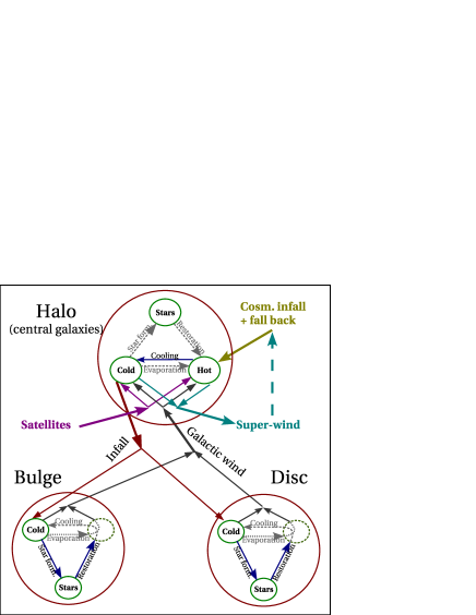
Figure 3: General scheme of mass flows in a model galaxy. The flows highlighted by dashed lines and gray colours are not used in the present version of the model. In particular, star formation (and then restoration and evaporation) in the halo is not active, while in bulge and disc components the evaporation and hot wind flows, as well as the restoration and cooling flows, are equated so as to leave the hot phase empty.

Mass flows

$\dot{M}_{\rm c,H}=\dot{M}_{\rm co,H}-\dot{M}_{\rm in,H}-\dot{M}_{\rm csw}+\dot{M}_{\rm cw,H}+\dot{M}_{\rm csat}$

$\dot{M}_{\rm h,H}=\dot{M}_{\rm cosm}-\dot{M}_{\rm co,H}-\dot{M}_{\rm hsw}+\dot{M}_{\rm hw,H}+\dot{M}_{\rm hsat}$

$\dot{M}_{\rm s,H}=0$

$\dot{M}_{\rm c,B}=\dot{M}_{\rm in,B}-\dot{M}_{\rm sf,B}+\dot{M}_{\rm rs,B}-\dot{M}_{\rm hw,B}-\dot{M}_{\rm cw,B}$

$\dot{M}_{\rm s,B}=\dot{M}_{\rm sf,B}-\dot{M}_{\rm rs,B}$

$\dot{M}_{\rm c,D}=\dot{M}_{\rm in,D}-\dot{M}_{\rm sf,D}+\dot{M}_{\rm rs,D}-\dot{M}_{\rm hw,D}-\dot{M}_{\rm cw,D}$

$\dot{M}_{\rm s,D}=\dot{M}_{\rm sf,D}-\dot{M}_{\rm rs,D}$

Energy Flows

$\dot{K}_{\rm H}=\dot{K}_{\rm co,H}-\dot{K}_{\rm in,H}-\dot{K}_{\rm csw}+\dot{K}_{\rm w,H}+\dot{K}_{\rm csat}-\dot{K}_{\rm ad}$

$\dot{E}_{\rm H}=\dot{E}_{\rm cosm}-\dot{E}_{\rm co,H}-\dot{E}_{\rm hsw}+\dot{E}_{\rm hw,H}+\dot{E}_{\rm hsat}-\dot{E}_{\rm ad}$

Metal Flows

$\dot{M}^{Z}_{\rm c,H}=\dot{M}^{Z}_{\rm co,H}-\dot{M}^{Z}_{\rm in,H}-\dot{M}^{Z}_{\rm csw}+\dot{M}^{Z}_{\rm cw,H}+\dot{M}^{Z}_{\rm csat}$

$\dot{M}^{Z}_{\rm h,H}=\dot{M}^{Z}_{\rm cosm}-\dot{M}^{Z}_{\rm co,H}-\dot{M}^{Z}_{\rm hsw}+\dot{M}^{Z}_{\rm hw,H}+\dot{M}^{Z}_{\rm hsat}$

$\dot{M}^{Z}_{\rm s,H}=0$

$\dot{M}^{Z}_{\rm c,B}=\dot{M}^{Z}_{\rm in,B}-\dot{M}^{Z}_{\rm sf,B}+\dot{M}^{Z}_{\rm rs,B}-\dot{M}^{Z}_{\rm hw,B}-\dot{M}^{Z}_{\rm cw,B}+\dot{M}^{Z}_{\rm yi,B}$

$\dot{M}^{Z}_{\rm s,B}=\dot{M}^{Z}_{\rm sf,B}-\dot{M}^{Z}_{\rm rs,B}$

$\dot{M}^{Z}_{\rm c,D}=\dot{M}^{Z}_{\rm in,D}-\dot{M}^{Z}_{\rm sf,D}+\dot{M}^{Z}_{\rm rs,D}-\dot{M}^{Z}_{\rm hw,D}-\dot{M}^{Z}_{\rm cw,D}+\dot{M}^{Z}_{\rm yi,D}$

$\dot{M}^{Z}_{\rm s,D}=\dot{M}^{Z}_{\rm sf,D}-\dot{M}^{Z}_{\rm rs,D}$

Ejected matter

$\dot{M}_{\rm c,E}=\dot{M}_{\rm csw}$

$\dot{K}_{\rm c,E}=\dot{K}_{\rm csw}$

$\dot{M}_{\rm h,E}=\dot{M}_{\rm hsw}$

$\dot{E}_{\rm h,E}=\dot{E}_{\rm hsw}$

$\dot{M}^{Z}_{\rm c,E}=\dot{M}^{Z}_{\rm csw}$

$\dot{M}^{Z}_{\rm h,E}=\dot{M}^{Z}_{\rm hsw}$

Black hole flows (equations 81)

$\dot{M}_{\rm BH}=\min(\dot{M}_{\rm visc}\,,\,M_{\rm BH}/t_{\rm Ed})$

$\dot{M}_{\rm resv}=\dot{M}_{\rm lowJ}-\dot{M}_{\rm BH}$

Cooling radius (equation 28)

$\dot{r}_{\rm cool}=(\dot{M}_{\rm co,H}-\dot{M}_{\rm hw,H})/(4\pi\rho_{g}(r_{\rm cool})r_{\rm cool}^{2})$

Table 1: The system of equations that is integrated by the code.

Flow	Comment	Reference
	Mass flows
$\dot{M}_{\rm co,H}$	cooling flow	eq. 23
$\dot{M}_{\rm in,H}$	infall from halo	eq. 31
$\dot{M}_{\rm csw}$	cold super-wind	eq. 42
$\dot{M}_{\rm cw,H}$	cold wind to halo	eq. 1
$\dot{M}_{\rm csat}$	cold wind from satellites	eq. 3
$\dot{M}_{\rm cosm}$	cosmological infall	eq. 19
$\dot{M}_{\rm hsw}$	hot super-wind	eq. 38
$\dot{M}_{\rm hw,H}$	hot wind to halo	eq. 1
$\dot{M}_{\rm hsat}$	hot wind from satellites	eq. 3
$\dot{M}_{\rm in,B}$	infall to bulge	eqs. 33, 35
$\dot{M}_{\rm sf,B}$	star formation in bulge	eq. 63
$\dot{M}_{\rm rs,B}$	restoration in bulge	eq. 63
$\dot{M}_{\rm hw,B}$	hot wind from bulge	eqs. 65, 73, 74
$\dot{M}_{\rm cw,B}$	cold wind from bulge	eqs. 71, 75
$\dot{M}_{\rm in,D}$	infall to disc	eqs. 34, 36
$\dot{M}_{\rm sf,D}$	star formation in disc	eq. 59
$\dot{M}_{\rm rs,D}$	restoration in disc	eq. 59
$\dot{M}_{\rm hw,D}$	hot wind from disc	eq. 59
$\dot{M}_{\rm cw,D}$	cold wind from disc	eq. 59
	Kinetic energy of cold halo gas
$\dot{K}_{\rm co,H}$	energy of cooling flow	eq. 25
$\dot{K}_{\rm in,H}$	energy lost by infall	eq. 32
$\dot{K}_{\rm csw}$	energy lost by cold super-wind	eq. 43
$\dot{K}_{\rm w,H}$	energy acquired by winds	eq. 61, 67, 72
$\dot{K}_{\rm csat}$	energy acquired by satellites	eq. 3
$\dot{K}_{\rm ad}$	adiabatic expansion	eq. 44
	Thermal energy of hot halo gas
$\dot{E}_{\rm cosm}$	shock-heating of infalling IGM	eq. 20
$\dot{E}_{\rm co,H}$	cooling of hot gas	eq. 24
$\dot{E}_{\rm hsw}$	energy lost by hot super-wind	eq. 39
$\dot{E}_{\rm hw,H}$	hot wind to halo	eqs. 60, 7.3, 83
$\dot{E}_{\rm hsat}$	hot wind from satellites	eq. 3
$\dot{E}_{\rm ad}$	adiabatic expansion	eq. 40
	Newly generated metals
$\dot{M}^{Z}_{\rm yi,B}$	new metals in bulge cold gas	eq. 78
$\dot{M}^{Z}_{\rm yi,D}$	new metals in disc cold gas	eq. 78
$\dot{M}^{Z}_{\rm hw,H}$	new metals injected to the halo	eq. 77
	BH flows
$\dot{M}_{\rm lowJ}$	loss of angular momentum	eq. 79
$\dot{M}_{\rm visc}$	viscous accretion rate	eq. 80

Table 2: Mass and energy flows in the system of equations (table 1). Metal flows are not reported.

2.4 Physical processes and flows

The present paper is dedicated to a detailed description of all the physical processes included in the code. Here we give only a global view of these processes with references to the section of the paper where they are described. We also report the system of equations that is integrated by the code, and a list of the mass, energy and metal flows.

Baryonic matter flows between the components and the phases as illustrated in figure 3. Within each component the three phases may exchange mass through the following flow terms:

• evaporation of gas from the cold to the hot phase ($\dot{M}_{\rm ev}$);

• cooling of gas from the hot to the cold phase ($\dot{M}_{\rm co}$);

• star formation from the cold to the star phase ($\dot{M}_{\rm sf}$);

• restoration from the star to the hot phase ($\dot{M}_{\rm rs}$).

As matter of fact, these flows are formally present in the code but they are never active at the same time. Indeed, in the halo component of central galaxies star formation (and then evaporation and restoration) are not active. In the bulge and disc components the hot phase is kept void by equating the restoration and cooling flow from the one hand, the evaporation and hot wind flow on the other hand; this is indicated in figure 3 by connecting, in the bulge and disc component, the arrows corresponding to the equated flows. In the following we will restrict ourselves to the flows that are used in the present formulation of the model, with the caveat that the other flows may be easily activated whenever required.

Baryonic matter flows between the components as follows:

• primordial gas flows to the halo together with the accreted DM mass (cosmological infall, $\dot{M}_{\rm cosm}$);

• cold gas infalls from the halo to the disc or bulge ($\dot{M}_{\rm in}$);

• cold and hot gas are expelled by the bulge or disc to the halo in a galactic wind ($\dot{M}_{\rm cw}$ and $\dot{M}_{\rm hw}$);

• both hot and cold gas are allowed to leave the halo in a galactic super-wind ($\dot{M}_{\rm hsw}$ and $\dot{M}_{\rm csw}$);

• this expelled material is allowed to get back to the halo together with the cosmological infall;

• winds from satellites are injected in the halo component of their central galaxy ($\dot{M}_{\rm csat}$ and $\dot{M}_{\rm hsat}$).

Mass conservation implies the following relations:

$$\dot{M}_{\rm in,H} = \dot{M}_{\rm in,B}+\dot{M}_{\rm in,D}$$

$$\dot{M}_{\rm cw,H} = \dot{M}_{\rm cw,B}+\dot{M}_{\rm cw,D}$$ (1)

$$\dot{M}_{\rm hw,H} = \dot{M}_{\rm hw,B}+\dot{M}_{\rm hw,D}$$

As illustrated above (section 2.2), in the cases of instabilities (disc instabilities and quasar-triggered galaxy winds), galaxy mergings, tidal stripping, tidal destruction and removal of halo baryonic component from new satellites, baryonic masses, energies and metals are moved between components and galaxies outside the integration routine. These flows are named in this paper external flows. It is worth noting that, as star formation in the halo is not allowed, stars flow to the halo component only through external flows (namely tidal stripping and galaxy mergings).

The system of equations integrated by the galaxy evolution code is reported in table 1. For all the equations, the suffixes c, h and s in the right hand sides denote the cold, hot and star phases. In all pedices the letters H, B, D and E following the comma denote the flows relative to the halo, bulge and disc components, and the matter ejected out of the DM halo by super-winds.

Table 2 gives a list of all mass flows, with a quick explanation and a reference to the equation where they are defined; metal flows follow trivially mass flows (see section 8) with the exception of the newly generated metals, so for sake of brevity we only report these in the table. Finally, table 3 gives the list of processes modeled in this paper, with reference to the relative section and the list of the related mass and energy flows.

Physical process implemented in the integration	Section	Flows modeled in that section
Galaxy winds from satellite galaxies	2.5	$\dot{M}_{\rm csat}$, $\dot{K}_{\rm csat}$, $\dot{M}_{\rm hsat}$, $\dot{E}_{\rm hsat}$
Hydrostatic equilibrium for the hot halo phase	5.1	$-$
Shock heating of cosmological infalling gas	5.2	$\dot{M}_{\rm cosm}$, $\dot{E}_{\rm cosm}$
Radiative cooling of hot halo gas	5.3	$\dot{M}_{\rm co,H}$, $\dot{E}_{\rm co,H}$, $\dot{K}_{\rm co,H}$
Infall of cold gas on the galaxy	5.4	$\dot{M}_{\rm in,H}$, $\dot{K}_{\rm in,H}$, $\dot{M}_{\rm in,B}$, $\dot{M}_{\rm in,D}$
Galaxy super-winds	5.5	$\dot{M}_{\rm hsw}$, $\dot{E}_{\rm hsw}$, $\dot{E}_{\rm ad}$, $\dot{M}_{\rm csw}$, $\dot{K}_{\rm csw}$, $\dot{K}_{\rm ad}$
Disc structure	6.1	$-$
Bulge structure	6.2	$-$
Star formation and feedback in discs	7.2	$\dot{M}_{\rm sf,D}$, $\dot{M}_{\rm rs,D}$, $\dot{M}_{\rm hw,D}$, $\dot{M}_{\rm cw,D}$, $\dot{E}_{\rm hw,H}$, $\dot{K}_{\rm w,H}$
Star formation and feedback in bulges	7.3	$\dot{M}_{\rm sf,B}$, $\dot{M}_{\rm rs,B}$, $\dot{M}_{\rm hw,B}$, $\dot{M}_{\rm cw,B}$, $\dot{E}_{\rm hw,H}$, $\dot{K}_{\rm w,H}$
Metal enrichment	8	$\dot{M}^{Z}_{\rm hw,H}$, $\dot{M}^{Z}_{\rm yi,B}$, $\dot{M}^{Z}_{\rm yi,D}$
Accretion onto BHs	9.1	$\dot{M}_{\rm visc}$, $\dot{M}_{\rm lowJ}$
AGN feedback	9.2	$\dot{E}_{\rm hw,H}$
Processes implemented as external flows	Section
Disc instabilities	6.1
Quasar-triggered galaxy winds	9.3
Decay of satellite orbits by dynamical friction	4.1
Tidal stripping at the periastron	4.1
Tidal destruction of satellites	4.1
Galaxy mergers	4.3
Stripping of halo component of satellites	2.5

Table 3: List of physical processes implemented in the code, with reference to the relevant section, and relative mass, energy and metal flows.

2.5 Super-winds and satellite galaxies

The matter ejected out of the DM halo by super-winds is collected into the variables denoted in table 1 by the “,E” pedix. After each integration interval these variables are stored in a vector, so as to be re-accreted at a later time together with the cosmological infall term; this is explained in section 5.5.

In the present version of the model, satellite galaxies do not retain their baryonic halo component. However, satellite galaxies continually produce galaxy winds as long as star formation is active. The related flows are given to the halo component of the main DM halo as follows. First, the (cold and hot) winds and superwinds flows are equated:

$$\dot{M}_{\rm csw} = \dot{M}_{\rm cw,H}$$

$$\dot{K}_{\rm csw} = \dot{K}_{\rm cw,H}$$

$$\dot{M}_{\rm hsw} = \dot{M}_{\rm hw,H}$$ (2)

$$\dot{E}_{\rm hsw} = \dot{E}_{\rm hw,H}$$

Then, at the end of the integration over the time interval the ejected matter is added to a vector aimed to contain the contribution of all the satellites to the halo component of the central galaxy. We call these vectors $M_{\rm csat}$, $M_{\rm hsat}$ and so on. The central galaxy is always evolved as the last one; when this happens the content of the satellite vectors is injected to the halo phase at a rate equal to the total mass or energy divided by the $\Delta t$ time interval:

$$\dot{M}_{\rm csat} = M_{\rm csat}/\Delta t$$

$$\dot{K}_{\rm csat} = \max(K_{\rm csat},M_{\rm csat}V_{\rm disp}^{2}/2)/\Delta t$$

$$\dot{M}_{\rm hsat} = M_{\rm hsat}/\Delta t$$ (3)

$$\dot{E}_{\rm hsat} = E_{\rm hsat}/\Delta t$$

It is worth noticing that the kinetic energy of the cold wind is recomputed using the velocity dispersion of the DM halo as long as this velocity is higher than the kinetic velocity of the cold ejected gas.

2.6 Initial conditions

At the appearance time all DM halos are assumed to be as large as 10 particles. All the bayons present in these primordial DM halos are assumed to be in the hot halo phase, whose thermal energy, acquired by gravitational shocks, is computed with the model described in section 5.2. An issue with this setting is the quick start of cooling in these initial halos. This is in part a numerical artifact due to the lack of sampling of the tree; if this were resolved with a smaller particle mass, the DM halo would then possibly contain some heating source at that time. To limit this resolution effect, it is assumed that the halos have just suffered a major merger at their appearance time, so that the onset of cooling is delayed by a few sound-crossing times (see section 5.2 for details). On the other hand, cooling in small halos is hampered by the ionizing background, and this is implemented (following Benson et al. 2002) by quenching cooling in all halos with circular velocities smaller than 50 km s^-1 (section 5.3).

Overcooling is connected to the very general problem of the stability of model predictions with respect to mass resolution. Appendix B presents a very simple convergence test of the model; the main conclusion is that model predictions do not converge and that the 50 km s^-1 cutoff motivated by the reionization guarantees that convergence is forced at low redshift and high masses. This opens a very delicate topic, which has rarely been addressed in the literature (see Hatton et al. 2003); we leave a deeper analysis and discussion to further work, and limit ourselves to pointing out which of the results presented here are more sensitive to mass resolution. In any case, as the lack of convergence regards star formation at very high redshift and faint galaxies, we can safely conclude that the building of bright galaxies does not depend strongly on mass resolution.

3 DM halos

3.1 DM merger trees

Figure 4: Example of ordering of the pinocchio merger trees. Circles with numbers denote DM progenitors, DM halos are denoted by their linking lists. In all the mergings shown in this picture, the DM halo coming from the left is more massive than that coming from the right.

As mentioned above, we use the pinocchio code to generate the merger trees. The use of pinocchio is motivated by its ability to give, even with modest computer resources, an adequate description of the hierarchical formation of DM halos, in excellent agreement with the results of N-body simulations (see also Zhao et al. 2003; Li, Mo & van der Bosch 2005); for instance, the mass function of DM halos is recovered to within a 5-10 per cent accuracy (Monaco et al. 2002a), while the mass function of progenitors of DM halos in a specified mass interval is recovered within a 10-20 per cent error (Taffoni et al. 2002). This code uses a scheme based on Lagrangian Perturbation Theory (Moutarde et al. 1991; Buchert & Ehlers 1993): starting from a Gaussian density contrast field sampled on a grid (very much similarly to the initial conditions of an N-body simulation) and smoothed over a set of smoothing radii, the earliest collapse time (the time at which the first orbit crossing takes place) is computed for each particle. Collapsed particles are then gathered into DM halos, where each halo is seeded by a peak of the inverse collapse time field. This procedure allows a detailed reconstruction of the DM halos, with known positions, velocities and angular momenta, and of their merger trees. The pinocchio merger trees are equivalent to those given by N-body simulations, with a further advantage (shared with the less accurate Extended Press & Schechter approach; see Bond et al. 1992; Lacey & Cole 1993) of a very fine time sampling that allows to track the merging times without being restricted to a fixed grid in time (or scale factor). Other notable differences with respect to N-body trees is the impossibility of pinocchio DM halos to decrease in mass, a condition which is not strictly valid for the N-body simulations. At variance with extended Press & Schechter merger trees, pinocchio allows for multiple mergers of DM halos.

The format of the pinocchio outputs (in the updated 2.1 version, available at http://adlibitum.oats.inaf.it/monaco/pinocchio/) are such that only the output at the final redshift is needed to reconstruct the merger trees of a realization, and from them compute the galaxy properties at all times. In pinocchio, each DM halo retains its identity even when it disappears by merging with another larger halo. The output files contain, for each DM halo that has ever existed with at least 10 particles, the following information: (i) ID number, (ii) ID of the halo it belongs to at the final redshift, (iii) linking list of the halos, (iv) ID of the halo it has merged with, (v) mass of the halo at the merging time, (vi) mass of the halo it has merged with (before merging) (vii) merging redshift, (viii) appearance redshift. Halos that exist at the final redshift have field (i) and (ii) equal, and merging redshift equal to -1; field (iv) is also set to -1, while field (v) contains the mass of the halo at the final redshift and field (vi) is 0.

Similarly to galform (Cole et al. 2000), the linking list provided by the 2.1 version of pinocchio is organized in such a way that merged halos are accessed so as to preserves chronological order. This is illustrated in the example of figure 4. Each time a halo appears from a peak, its linking list points to itself. Suppose now that halo 1 merges with the smaller halo 2 at $z_{\rm merge}$=10, and that both halos have no substructure. Then the linking list is updated so that halo 1 points to halo 2 and vice-versa. At $z_{\rm merge}$=5.3 halo 1 (which contains halo 2 as a substructure) merges with halo 3, which has no substructure. Then the last halo of the chain, halo 2, is linked to halo 3, and this back to halo 1. Halos 5 and 6 merge at $z_{\rm merge}$=7.5, and their fate is similar to halos 1 and 2. Halo 5 then merges with the larger halo 4 at $z_{\rm merge}$=4.1; in this case halo 4 does not link directly to halo 5, which is put at the end of the chain, but to halo 6. At $z_{\rm merge}$=2.1 halos 1 and 4 merge. In this case, the last element of the chain of halo 1 (halo 3) is linked to the second of the chain of halo 4 (halo 6). The final sequence is then 1-2-3-6-5-4. In more general terms, the two groups are linked in the following order: first the chain of the surviving DM halo, then the chain of the disappearing one, with the first element (the main halo before merging) put as last. It is clear that, starting from the second element of the final chain, two subsequent events are always accessed in chronological order. This does not imply a strict chronological order of all the mergings: in our example halo 3 ($z_{\rm merge}$=5.3) is accessed before halo 6 ($z_{\rm merge}$=7.5), but the two event are on independent branches of the tree.

3.2 DM halo properties

The physical properties of the DM halos (which are not predicted by pinocchio) are computed at each integration time-step (see figure 2) as follows. The density profile of the DM halo is assumed to follow Navarro, Frenk & White (1996; hereafter NFW), according to which a halo with a virial radius $r_{\rm H}$ is characterized by a scale radius $r_{s}$ and a concentration $c_{\rm nfw}=r_{\rm H}/r_{s}$. Defining the quantity $\delta_{c}\equiv 200c_{\rm nfw}^{3}(1+c_{\rm nfw})/(3(1+c_{\rm nfw})\ln(1+c_{\rm nfw})-c_{\rm nfw})$, the NFW profile of a halo at redshift $z$ is:

$$\rho_{\rm DM}(r)=\rho_{c}(z)\frac{\delta_{c}}{c_{\rm nfw}x(1+c_{\rm nfw}x)^{2}}\,,$$ (4)

where $\rho_{c}(z)$ is the critical density at the redshift $z$ and $x\equiv r/r_{s}$. The virial radius $r_{\rm H}$ of a halo of circular velocity $V_{\rm H}$ is computed assuming that its average density its 200 times the critical density (see, e.g., Mo, Mao & White 1998):

$$\begin{array}[]{lll}V_{\rm H}&=&(10M_{\rm H}GH(z))^{1/3}\\ r_{\rm H}&=&V_{\rm H}/10H(z)\end{array}$$ (5)

where $M_{\rm H}$ is the total halo mass and $H(z)$ is the Hubble constant at $z$.

The concentration $c_{\rm nfw}$ is computed, as a function of $M_{\rm H}$ and $z$, following Eke, Navarro & Steinmetz (2001). Given the mass $M_{\rm H}$, redshift $z$ and concentration $c_{\rm nfw}$ we compute the gravitational binding energy of the halo ($U_{\rm H}=\int\rho\Phi d^{3}r$) as:

$$U_{\rm H}=\frac{GM_{\rm H}^{2}}{r_{\rm H}}\delta_{c}^{2}\left(\ln^{2}(1+c_{\rm nfw})-\frac{c_{\rm nfw}^{2}}{1+c_{\rm nfw}}\right)\;.$$ (6)

From it and the virial theorem the velocity dispersion of the halo (such that the total kinetic energy of halo particles is $M_{\rm H}V_{\rm disp}^{2}/2=-U_{\rm H}/2$) can be computed as:

$$V_{\rm disp}=\sqrt{-U_{\rm H}/M_{\rm H}}$$ (7)

If $\lambda$ is the spin parameter of the DM halo, its specific angular momentum is computed as:

$$\frac{J_{\rm H}}{M_{\rm H}}=GM_{\rm H}\lambda\sqrt{-0.5U_{\rm H}/M_{\rm H}}\,.$$ (8)

The DM halo parameters ($M_{\rm H}$, $c_{\rm nfw}$, $r_{h}$, $V_{\rm H}$, $U_{\rm H}$, $J_{\rm H}$) are re-computed at each time-step along the integration.

The spin parameter $\lambda$ of DM halos is in principle provided by pinocchio, which is able to predicted the angular momenta of halos. The predicted momenta show some (modest) degree of correlation with those of simulated halos (the spin directions tend to be loosely aligned within 60^∘), and their statistics is reproduced at the cost of adding free parameters (Monaco et al. 2002b). While even a modest correlation with the N-body solution is an advantage with respect to drawing random numbers, the complications involved in reconstructing the spin history of halos weight more than any possible practical advantage. As a consequence, we prefer to randomly assign a $\lambda$ value to each DM halo, drawing it from the log-normal distribution:

$$P_{\log\lambda}(\log\lambda)d\log\lambda=\frac{1}{\sqrt{2\pi}\theta}\exp\left(-\frac{(\log\lambda-\log\lambda_{0})^{2}}{2\theta^{2}}\right)$$ (9)

where we use values $\lambda_{0}=0.05$ and $\theta=0.3$ (Cole et al. 2000 use the slightly lower value of 0.23 for $\theta$; we follow Monaco, Salucci and Danese 2000 using 0.3, which is a better fit to many spin distributions available in the literature and cited in that paper). As explained in section 6.1, a variation of $\lambda$ with time (for instance at major mergers) creates problems with the model of disc structure. To avoid these problems, the $\lambda$ parameters are held constant during the evolution of each halo. This does not imply a constant specific angular momentum for the halos, as both $M_{\rm H}$ and $U_{\rm H}$ in equation 8 change with time.

As for DM satellites, it is assumed that their properties (mass, scale radius, concentration) remain constant after their merging. Satellites are however subject to tidal stripping, as explained in section 4.1. Tidal stripping is only taken into account in two cases: to strip baryonic mass from discs and bulges, in case of extreme stripping, and to compute the merging time for substructure after a merger. In all the other cases the unstripped mass of the satellite is used.

4 Galaxy mergers, destruction and stripping

4.1 Dynamical evolution of satellites

The computation of merging times for satellites follows the model of Taffoni et al. (2003). In the simplest case, two DM halos without substructure merge, so that the smaller halo becomes a satellite of the larger one. The properties of the two halos at the merging time are computed as explained in section 3.2, and the subsequent evolution of the main halo is neglected (up to the next major merger). The orbital parameters are extracted at random from suitable distributions, in particular the eccentricity of the orbit (defined as $\epsilon=J/J_{\rm cir}$, where $J$ is the initial angular momentum of the orbit and $J_{\rm cir}$ the angular momentum of a circular orbit with the same energy) is extracted from a Gaussian distribution with mean 0.7 and variance 0.2, while the energy of the orbit, parameterized with $x_{c}$ (defined as $x_{c}=r_{c}/r_{\rm H}$, where $r_{c}$ is the radius of a circular orbit with the same energy and $r_{\rm H}$ the halo radius) is taken to be 0.5 for all orbits. These numbers are suggested by an analysis of the orbit of satellites in a high-resolution N-body simulation (Ghigna, private communication), and are slightly different from the results of Tormen (1997), who found a lower value (0.5) for $\epsilon$ and did not publish the distribution of $x_{c}$ (he gave the distribution of the radius of the first periastron, but this quantity is affected by dynamical friction in a subtle way); however, we have verified that choosing Tormen’s value does not induce significant differences in the results. The choice of $x_{c}=0.5$ is equivalent to the implicit choice of Somerville & Primack (1999), who use a flat distribution for $\epsilon$, while Cole et al. (2000) extract a combination of the two parameters, $\epsilon^{0.78}x_{c}^{2}$, from a log-normal distribution and Kauffmann et al. (1999) extract $\epsilon$ again from a flat distribution and use $x_{c}=1$.

Galaxy mergings are due to the decay of the orbit of their host DM satellite by dynamical friction; in this scheme galaxy satellites can only merge with their central galaxy. Tidal shocks can lead to a complete disruption of satellites; in these rather unlikely events all the (dark and baryonic) matter of the satellite is dispersed into the halo of the central galaxy. Taffoni et al. (2003) give fitting formulae, accurate to the 15% level, for the merging and destruction times for substructures that take into account dynamical friction, mass loss by tidal stripping and tidal shocks. We use a slightly different version of those fitting formule, with updated parameters that slightly improve the fits to simulations; these are given in appendix A.

Though the merger and disruption times of Taffoni et al. (2003) include a rather sophisticated treatment of tidal stripping, we implement this process at a very simple level. Tidal stripping is applied at the first periastron of the satellite. The tidal radius is computed as the radius at which the density of the unperturbed satellite is equal to the density of the main DM halo at the periastron. All the mass external to the tidal radius is then considered as unbound from the satellite. However, while the stripping radius is recorded, the halo mass is not updated but kept fixed in the following evolution. Indeed, disc structure (see section 6.1) is computed using the DM halo profile at of the satellite at its merger time (i.e. ignoring stripping), while the recomputation of merging times after a major merger is done using the stripped mass.

Tidal stripping at periastron affects also the fraction of stellar and gas mass of disc and bulge that lies beyond the tidal radius. Notice that, for simplicity, neither the DM halo nor the disc and bulge are assumed to be perturbed by this process beyond the decrease of mass. Within the model structure, stripping is applied outside the numerical integration, so it is an external flow (section 2.2).

In the more general case of two substructured halos that merge, we distinguish between major and minor mergers as follows:

$${\rm Major\ merger\ of\ DM\ halos:}\ \ \ \ M_{\rm sat}/M_{\rm main}>f_{\rm hmm}$$ (10)

(we recall that the main DM halo includes the satellite). N-body simulations show that when this condition, with $f_{\rm hmm}\simeq 0.2$, is satisfied the perturbation induced by the satellite leads to a reshuffling of all the orbits. At a major merger we then re-extract the orbital parameters and re-compute the merger and destruction times for all the satellites of the main DM halo, as if they just entered the halo. As a consequence, some galaxies near to their merging time can be moved to a different orbit that does not lead to merging, while some other galaxies can suffer tidal stripping more than once. Clearly the re-computation of the merging and destruction times for a substructure may not be very accurate, especially for satellites that have suffered strong mass loss. In this case we keep the scale radius and concentration of the satellite fixed, but use (as mentioned above) the stripped mass to compute the merging and destruction times. As these times are rather long for small satellites, the final results is that the galaxies just don’t merge and the accuracy of the prediction is not an issue.

Minor mergers do not influence the evolution of the satellites of the main DM halo, but do affect the satellites of the smaller DM halo (going itself to become a satellite), for which there is no difference between minor and major merger.

4.2 Galaxy merger trees

The galaxy merger trees are constructed, analogously to the DM halo merger trees, by specifying for each galaxy (i) the galaxy where its stars lie at the the final time, (ii) the merging redshift, (iii) the galaxy it has merged with, (iv) a linking list for the merged galaxies, (v) and (vi) the masses of each pair of merged galaxies. Destroyed galaxies are recorded by assigning a negative value to field (i). The construction of galaxy trees is performed as follows: at each halo merger the merging and destruction times for the galaxies are computed (section 4.1), then the galaxies are merged or destroyed at that time if the DM halo they belong to has not been involved in a major merger nor has become a satellite in the meantime. While multiple mergers are allowed by pinocchio, galaxy mergers are all binary.

4.3 Galaxy mergers

When two galaxies merge, their fate depends again on the ratio of their masses. Major mergers of galaxies are defined as:

$${\rm Major\ merger\ of\ galaxies:}\ \ \ \ M_{\rm sat}/M_{\rm cen}>f_{\rm gmm}$$ (11)

where the parameter $f_{\rm gmm}$ is suggested by simulations to take a value of 0.3 (Kauffmann et al. 1999; Cole et al. 2000). In this specific case baryonic masses are used (i.e. the mass in hot, cold and star phases of the bulge and halo components), and the central galaxy does not include the satellite, so this condition is similar to that of equation 10 with a value of 0.25. While the condition on DM halos can be computed directly from the pinocchio trees and without running the galaxy evolution code, the condition of equation 11 must be computed at the merger time, after the evolution code has determined the baryonic galaxy masses.

At minor galaxy mergers the whole satellite is added to the bulge, while the disc remains unaffected. This is at variance with Cole et al. (2000), that give the stars to the bulge and the gas to the disc. Their choice is however questionable, as the dissipative matter is more likely to go to the bulge; this is why we prefer to give everything to the bulge. A more accurate solution of this problem will clearly depend on the orbit of the merger, but an implementation of these second-order effects would require a large set of N-body simulations to quantify and parameterize these dependences. In any case, our tests have revealed no strong difference between the two cases (see section 6.2 for more comments).

At a major galaxy merger all the gas and stars of the two merging galaxies are given to the bulge of the central one. Due to the shorter time-scale of star formation in bulges (see section 7), a starburst is stimulated by the presence of gas in the bulge component.

Stripping and galaxy destruction (which is an extreme stripping event) bring stars to the halo of the central galaxy. As star formation in the halo is inactive, this is the main way to have stars to the halo. We anticipate that this mechanism is not very effective in galaxy clusters, where only a few per cent of the stellar mass is stripped to the halo, at variance with the 10-40 per cent found in observed clusters (Feldmeier et al. 2003; Arnaboldi et al. 2003; Gal-Yam et al. 2003; Zibetti et al. 2005). Murante et al. (2004; 2006) have performed hydro simulations to address this problem, coming to the conclusion that the high fraction of cluster stars can be reproduced, but the main mechanism is not tidal stripping but violent relaxation in major mergers. Very recently, Monaco et al. (2006), based on morgana and on the N-body results of Murante et al. (2006), proposed that the construction of the stellar diffuse component of galaxy clusters, i.e. the halo star phase, is related to the apparent lack of evolution of the most massive galaxies since $z=1$. They showed that the evolution driven by galaxy mergers alone is larger than what is observed in large galaxy samples, and that this discrepancy can be solved if a fair fraction of stars is scattered to the halo star component at each merger. However, to reproduce the observed increase of the stellar diffuse component with halo mass, the fraction of scattered stars must depend strongly on the properties of the DM halo and of the merging galaxies. This dependence should be provided by simulations, but this is a work in progress. In this paper we simply assume that a fraction $f_{\rm scatter}$ of the star mass of the merging galaxies is scattered to the halo at each major merging. With this simple rule we are able to produce a low fraction of halo stars in galactic halos and a higher one in galaxy cluster.

Interactions between satellites, like binary mergers, flybies (that stimulate star formation) or galaxy harassment (Moore et al. 1996) are not included at the moment. We know that these events can have an impact on the evolution of galaxies (Somerville & Primack 1999; Balland, Devriendt & Silk 2003; Menci et al. 2004) and AGNs (Cavaliere & Vittorini 2000). We plan to introduce such events in the future.

5 Halo gas

5.1 Equilibrium model for the hot phase

The hot halo phase is assumed to be (i) spherical, (ii) in hydrostatic equilibrium in an NFW halo (Suto, Sasaki & Makino 1998), (iii) filling the volume from a cooling radius $r_{\rm cool}$ to the virial radius $r_{\rm H}$, (iv) pressure-balanced both at $r_{\rm cool}$ and $r_{\rm H}$, (v) described by a polytropic equation of state with index ${\gamma_{\rm p}}$, a parameter that is observed to take a value of about 1.2 (see, e.g., De Grandi & Molendi 2002); we use the best-fit value of 1.15. The equilibrium configuration of the hot halo gas is computed at each time step as described below, under the assumption that in the absence of major mergers the gas re-adjusts quasi-statically to the new equilibrium configuration. We do not assume that the thermal energy $E_{\rm H}$ of the hot halo phase is a fixed fraction of the virial energy; on the contrary, we follow its evolution through the equation given in table 1. This is done to incorporate the response of the hot halo phase to the thermal feedback from galaxies. Under the assumptions given above, the constraints on the profile are then the mass and thermal energy of the gas.

The equation of hydrostatic equilibrium:

$$\frac{dP_{g}}{dr}=-G\frac{\rho_{g}M_{\rm H}(<r)}{r^{2}}$$ (12)

(where $P$ is the gas pressure, $r$ is the radius, $M_{\rm H}(<r)$ is the halo mass within $r$ and $\rho_{g}$ the gas density) is easily solved in the case of an NFW density profile (equation 4). The solution is:

$$\rho_{g}(r) = \rho_{g0}\left(1-a\left(1-\frac{\ln(1+c_{\rm nfw}x)}{c_{\rm nfw}}\right)\right)^{1/(\gamma_{p}-1)}$$

$$P_{g}(r) = P_{g0}\left(1-a\left(1-\frac{\ln(1+c_{\rm nfw}x)}{c_{\rm nfw}}\right)\right)^{\gamma_{p}/(\gamma_{p}-1)}$$ (13)

$$T_{g}(r) = T_{g0}\left(1-a\left(1-\frac{\ln(1+c_{\rm nfw}x)}{c_{\rm nfw}}\right)\right)$$

Defining the virial temperature of the halo as $T_{\rm vir}=\mu_{\rm hot}m_{p}V_{c}^{2}/3k$ (where $\mu_{\rm hot}=4/(8-5Y-6Z)$ is the mean molecular weight of the hot gas; $Z=M^{Z}_{\rm h,H}/M_{\rm h,H}$ is the metallicity of the hot halo gas and $Y$ assumes the solar value of 0.25), $\eta=T_{g}(r)/T_{\rm vir}$ and $\eta_{0}$ its extrapolation at $r=0$, the constant $a$ is defined as:

$$a=\frac{\gamma_{p}-1}{\gamma_{p}}\frac{3}{\eta_{0}}\frac{c_{\rm nfw}(1+c_{\rm nfw})}{(1+c_{\rm nfw})\ln(1+c_{\rm nfw})-c_{\rm nfw}}$$ (14)

The constants $T_{g0}$, $\rho_{g0}$ and $P_{g0}$ are defined as the extrapolation of the density and temperature profiles to $r=0$, even though the gas is assumed to be present only beyond $r_{\rm cool}$. As mentioned above, they are fixed by requiring that the total mass and energy of the gas correspond to $M_{\rm h,H}$ and $E_{\rm h,H}$. The first condition can be solved explicitly if the energy is specified. Calling ${\cal I}$ the integral:

$${\cal I}(\alpha)=\int_{r_{\rm cool}/r_{s}}^{c_{\rm nfw}}\left(1-a\left(1-\frac{\ln(1+t)}{t}\right)\right)^{\alpha}t^{2}dt$$ (15)

(where for simplicity we declare only the dependence on the $\alpha$ exponent) we have:

$$\rho_{g0}=\frac{M_{\rm h,H}}{4\pi r_{s}^{3}}\times\frac{1}{{\cal I}(1/(\gamma_{p}-1))}$$ (16)

The second condition is:

$$E_{\rm h,H}=\frac{6\pi kT_{g0}\rho_{g0}r_{s}^{3}}{\mu_{\rm hot}m_{p}}\times{\cal I}(\gamma_{p}/(\gamma_{p}-1))$$ (17)

This equation cannot be solved explicitly, as the coefficient $a$ depends on the energy itself through $\eta_{0}$. To find a solution to these two equations it is necessary to use an iterative algorithm. As a consequence, the computation of the two integrals contained in equations 16 and 17 is the most time-consuming computation of the whole code. A dramatic speed-up (at the cost of a negligible error) is obtained by computing the integrals in a grid of values of $a$, $r$ and $\gamma_{p}$; the solution is then found by linearly interpolating the table.

The function $1-a(1-\ln(1+c_{\rm nfw}x)/c_{\rm nfw})$ in equations 13 becomes negative at large radii. In this case density, pressure and temperature are not defined. Usually this happens beyond the virial radius $r_{\rm H}$, unless the central temperature is lower than the following limit:

$$\eta_{0}<3\frac{\gamma_{p}-1}{\gamma_{p}}\frac{c_{\rm nfw}-\ln(1+c_{\rm nfw})}{\ln(1+c_{\rm nfw})-c_{\rm nfw}/(1+c_{\rm nfw})}$$ (18)

This condition can be met at high redshift, when $c_{\rm nfw}$-values are high. In this case no gas is assumed to be present beyond the point of zero density, so that the gas is bound to the inner part of the halo and its pressure at the virial radius is null.

This model for the hot halo gas is very similar to that proposed by Ostriker, Bode & Babul (2005) to model the hot component of galaxy clusters, with two remarkable differences: first, they do not follow cooling, so the hot gas is present since $r=0$, instead of $r=r_{\rm cool}$. Clearly this does not make any difference in cases like galaxy clusters without cool cores, where $r_{\rm cool}\simeq 0$. Second, they assume an external pressure, computed on the basis of a fiducial infall velocity of cold gas, and extrapolate the gas profile until its thermal pressure equals the external one. This implies that the hot gas can extend beyond the virial radius. Our choice is to remove this outlier gas, and this allows to describe galaxy super-winds (section 5.5). Clearly the two criteria should be equivalent in the case of a small cooling radius and a thermal energy roughly similar to the virial one; we plan to deepen this point and to compare the predicted properties of the hot halo gas with simulations in the future.

5.2 Shock heating

The equilibrium model does not specify the amount of thermal energy of the hot gas. This is acquired by the infalling gas through shocks. The cosmological infall mass flow is computed by linearly interpolating the DM halo mass between the branch ends (whose distance in time is $\Delta t$) and assuming that a fraction $\Omega_{b}/\Omega_{0}$ of that mass is in IGM:

$$\dot{M}_{\rm cosm}=\frac{\Omega_{b}}{\Omega_{0}}\frac{\Delta M_{\rm H}}{\Delta t}$$ (19)

We then assume that this gas acquires an energy equal to $f_{\rm shock}$ times that suggested by the virial theorem:

$$\dot{E}_{\rm cosm}=f_{\rm shock}(-0.5\,U_{\rm H})\dot{M}_{\rm cosm}/M_{\rm H}$$ (20)

where the binding energy of the halo $U_{\rm H}$ is given by equation 6. The parameter $f_{\rm shock}$ is suggested by hydro simulations to be slightly higher than 1 (Wu, Fabian & Nulsen 2000). We adopt a value of 1.2.

A similar heating is applied in the following external flows:

• the hot gas contained in the DM halos at the appearance time (see section 2.6);

• the hot halo gas of satellite DM halos at their merging time’

• the hot halo gas at major mergers.

In all these cases:

$$E_{\rm H}=f_{\rm shock}(-0.5\,U_{\rm H})M_{\rm h,H}/M_{\rm H}$$ (21)

Hydro simulations suggest that any cold gas present in the halo is re-heated by shocks during a major merger. Accordingly, we allow shock-heating to affect also the cold halo phase at major mergers. This option is active in all the results presented here, but can be switched off on request.

Cases (ii) and (iii) refer to gravitational heating due to merging events. This heating is of course not instantaneous; the energy is redistributed to the whole halo gas in a few crossing times. This behaviour is implemented by quenching cooling for a number $n_{\rm quench}$ of crossing times $r_{\rm H}/V_{\rm H}$; after the quenching (which ends at some time $t_{q}$), the cooling flow is allowed to start gradually as $\exp\{-[r_{\rm H}/V_{\rm H}(t-t_{q})]^{2}\}$. The parameter $n_{\rm quench}$ is very important to control the cooling of gas, especially at high redshift. The same quenching is applied to DM halos at their appearance time (section 2.6); it amounts to assuming that the appearing halos have just formed by a major merger.

Using hydro simulations, some authors (Kravtsov 2003; Keres et al. 2005) have recently pointed out that cold gas can flow directly to the core of small-mass halos at high redshift by radiating very quickly the energy acquired by shocks. Following this idea, Dekel & Birnboim (2006; see also Cattaneo et al. 2006) have proposed that this lack of shock heating is a likely responsible for the observed transition in the behaviour from dwarf to bright galaxies. Besides, Croton et al. (2006) implement this idea by equating the infall mass flow with the cosmological infall one in the infall-dominated halos. A similar view is taken by Bower et al. (2006), who suppose that a short cooling time prevents the formation of a hydrostatic hot halo phase. These considerations question the validity of the shock heating and hydrostatic equilibrium hypotheses in infall-dominated halos; however, these are also the cases where the infall of gas on the galaxy does not depend much on the cooling time, so we choose to retain these hypotheses as they are accurate in the cases where they are most relevant.

5.3 Cooling

The cooling radius is defined as the radius within which the hot halo gas has cooled down. In most semi-analytic models the hot gas profile is computed at a major merger; the time-dependent cooling radius is then computed as the radius at which the cooling time of a gas shell is equal to the time since the merger. In the present model the cooling radius is instead treated as a dynamical variable. This allows to re-compute the gas profile at each time-step, and to incorporate the heating effect of the hot wind coming from the central galaxy.

The cooling rate of a shell of gas of width $\Delta r$ at a radius $r$ is computed as:

$$\Delta\dot{M}_{\rm co,H}(r)=\frac{\Delta M_{\rm h,H}(r)}{t_{\rm cool}(r)}\,,$$ (22)

where $\Delta M_{\rm h,H}=4\pi r^{2}\rho_{g}(r)\Delta r$ is the shell mass and $t_{\rm cool}(r)=3kT_{g}(r)\mu_{\rm hot}m_{p}/2\rho_{g}(r)\Lambda_{\rm cool}(T_{g}(r))$ is the cooling time at radius $r$. For the cooling function $\Lambda_{\rm cool}$, we use the metallicity-dependent function tabulated by Sutherland & Dopita (1993). The cooling time depends on density and temperature, but the density dependence is by far stronger, both intrinsically and because the temperature profile is much shallower than the gradient profile. So the integration in $r$ can be performed by assuming $T_{g}(r)\simeq T_{g}(r_{\rm cool})$. The resulting cooling flow is:

$$\dot{M}_{\rm co,H}=\frac{4\pi r_{s}^{3}\rho_{g0}}{t_{\rm cool,0}}\times{\cal I}(2/(\gamma_{p}-1))$$ (23)

where ${\cal I}$ is defined in equation 15. In this equation the cooling time $t_{\rm cool,0}$ is computed using $\rho_{g0}$ for the density (the dependence of density on radius is taken into account by the integrand), and $T_{g}(r_{\rm cool})$ for the temperature, as explained above. Analogously to the integrals of equations 16 and 17, the integral in equation 23 is computed on a grid of parameter values and then estimated by linear interpolation on the table. The rate of energy loss by cooling is computed analogously:

$$\dot{E}_{\rm co,H}=\frac{3kT_{g}(r_{\rm cool})}{2\mu_{\rm hot}m_{p}}\frac{4\pi r_{s}^{3}\rho_{g0}}{t_{\rm cool,0}}\times{\cal I}(2/(\gamma_{p}-1))$$ (24)

The cooled gas carries with it a kinetic energy:

$$\dot{K}_{\rm co,H}=\frac{1}{2}\dot{M}_{\rm co,H}V_{\rm disp}^{2}$$ (25)

where $V_{\rm disp}$ is the velocity dispersion of the DM halo defined in equation 7.

When a heating source is present, these two terms behave differently. While the energy radiated away by the hot gas at a given density and temperature does not change, the amount of cooled mass depends on how much of this energy is replaced by the heating source. We then compute the cooling time as:

$$t_{\rm cool,0}=\frac{3kT_{g}(r_{\rm cool})\mu_{\rm hot}m_{p}}{2\rho_{g0}(\Lambda_{\rm cool}-\Gamma_{\rm heat})}$$ (26)

This cooling time is used in equation 23 to compute the mass cooling flow. A negative value implies a net heating of the source, in which case the mass cooling flow $\dot{M}_{\rm co,H}$ (but not $\dot{E}_{\rm co,H}$) is set to zero.

The source of heating is the central galaxy, which hampers cooling through the hot wind energy flow, $\dot{E}_{\rm hw,H}$. This flow carries the energy produced by SNe, both in the bulge and in the disc, and by the AGN. Satellites instead are assumed to orbit on average in the external regions, so that the energy contributed by their winds is injected beyond the cooling radius and does not interact directly with the cooling flow. To compute the heating term it is necessary to specify how this heating is distributed. For simplicity we assume that heating and cooling affect the same gas mass $4\pi r_{s}^{3}\rho_{g0}{\cal I}(2/(\gamma_{p}-1))$, i.e. the inner shell at $r_{\rm cool}$ that is effectively cooling. The heating term is then computed as:

$$\Gamma_{\rm heat}=\frac{\dot{E}_{\rm hw,H}}{4\pi r_{s}^{3}{\cal I}(2/(\gamma_{p}-1))}\left(\frac{\mu_{\rm hot}m_{p}}{\rho_{g0}}\right)^{2}$$ (27)

Once the cooling and heating sources are fixed, the evolution of the cooling radius is computed by inverting the usual relation, $\dot{M}_{\rm co,H}=-4\pi\rho_{g}r_{\rm cool}^{2}dr_{\rm cool}/dt$, taking into account that the hot wind mass flow $\dot{M}_{\rm hw,H}$ is adding to the hot halo phase at the cooling radius:

$$\dot{r}_{\rm cool}=\frac{\dot{M}_{\rm co,H}-\dot{M}_{\rm hw,H}}{4\pi\rho_{g}(r_{\rm cool})r_{\rm cool}^{2}}\,.$$ (28)

In this way, the cooling radius decreases if the hot wind term overtakes the cooling term.

Equation 28 shows that the cooling radius should not vanish. Moreover, in the case of very strong cooling flows the Runge-Kutta integrator may try some calls with $r_{\rm cool}>r_{\rm H}$, giving rise to numerical problems. The cooling radius is then forced to lie between a small value (taken to be 0.01 times the scale radius $r_{\rm s}$) and 90 per cent of the virial radius $r_{\rm H}$. This is done by gradually setting $\dot{r}_{\rm cool}$ to zero when the limits are approached. The presence of a small lower limit for $r_{\rm cool}$ does not influence the results, because of the flat density profile in the central regions. The upper limit can instead influence significantly the behaviour of cooling, but this happens when most of the hot gas has already cooled, a situation in which a precise modeling is not very important and the validity of the model itself is more doubtful (see the discussion in section 5.1).

The existence of a “cooling hole” at the centre of the halo requires that, as we assumed in section 5.1, pressure is balanced at $r_{\rm cool}$. However, this assumption is clearly unphysical, as the cooled gas cannot give sufficient pressure support, so this assumption will work only as long as $\dot{r}_{\rm cool}>c_{s}$, where $c_{s}$ is the sound speed of the hot gas. In general, the gas at $r_{\rm cool}$ will be pushed toward the centre by its pressure. This can be modeled very simply as follows:

$$\dot{r}_{\rm cool}^{\prime}=\dot{r}_{\rm cool}-c_{s}$$ (29)

We have noticed that this feature induces an excessive and unphysical degree of cooling in the later stages of evolution, when, due to the decreasing temperature gradient, the residual thermal energy of the gas gets lower than the virial energy. To avoid it we consider the sound speed term only when the gas thermal energy $E_{\rm h,H}$ is higher than the virial value. This term is included on request, and is used in the results presented here.

Finally, after reionization the ionizing background is likely to prevent the cooling of any halo whose circular velocity is smaller than $\sim$50 km s^-1. As suggested by Benson et al. (2002), to mimic the effect of the UV background we simply suppress any cooling in all halos with $V_{c}<50$ km s^-1.

5.4 Infall

The dynamical time of the halo at a radius $r$ is defined as the time required by a mass particle to free-fall to the centre:

$$t_{\rm dyn}(r)=\frac{1}{\sqrt{2}V_{c}}\left(\frac{3\delta_{c}}{200c_{\rm nfw}^{2}}\right)^{-1/2}r_{s}$$

$$\times\int_{0}^{r/r_{s}}\left[\frac{\ln(1+y)}{y}-\frac{\ln(1+r/r_{s})}{r/r_{s}}\right]^{-1/2}\,dy$$

The cold phase is unstable to collapse and flows to the central galaxy. Starting with White & Frenk (1991), many semi-analytic codes, at variance with morgana, unify the processes of cooling and infall by computing an infall radius for the gas as the radius at which the infall time of a gas shell is equal to the time since last major merger, then using the smallest between the cooling and infall radii to compute the cooling flow. This choice implies an assumption of no difference between the hot halo gas and the cooled gas that is infalling toward the central galaxy. The hot wind ejected by a galaxy acts preferentially on the most pervasive hot phase, affecting in a much weaker way the cold infalling gas, which naturally fragments into clouds with a low covering factor. So, we deem that treating the infalling gas as belonging to a different phase is a step forward in the physical description of galaxy formation, especially in those infall-dominated halos where a high fraction of halo gas is in the cold phase. As a matter of fact, the recipe by Croton et al. (2006) discussed above (section 5.2) goes in the same direction, because with their assumption of $\dot{M}_{\rm cosmo}=\dot{M}_{\rm in,H}$ (valid for infall-dominated halos) the cooled gas is not affected by feedback.

The cold gas is let infall to the central galaxy on a number $n_{\rm dyn}$ of dynamical times computed at the cooling radius $r_{\rm cool}$:

$$\dot{M}_{\rm in,H}=\frac{M_{\rm c,H}}{n_{\rm dyn}t_{\rm dyn}(r_{\rm cool})}$$ (31)

The corresponding loss of kinetic energy is:

$$\dot{K}_{\rm in,H}=\frac{K_{\rm H}}{n_{\rm dyn}t_{\rm dyn}(r_{\rm cool})}$$ (32)

The infalling cold gas is distributed between the disc and the bulge as follows. As a first option, all the infalling gas is given to the disc, under the assumption that it has the same specific angular momentum as the DM halo:

$$\dot{M}_{\rm in,B} = 0$$ (33)

$$\dot{M}_{\rm in,D} = \dot{M}_{\rm in,H}$$ (34)

In presence of a significant or dominant bulge the formation of such a disc by infall implies that the bulge has no influence on it, even when a large fraction of it is embedded in the bulge. This is a rather strong assumption, as the hot pressurized phase pervading the bulge (section 7.3) can lead to significant loss of angular momentum of the gas by ram pressure. Then, as a second option we let gas infall on the bulge by a fraction equal to the mass of the disc contained within the half-mass radius of the bulge:

$$\dot{M}_{\rm in,B} = \dot{M}_{\rm in,H}\times\left[1-\exp\left(-\frac{R_{\rm B}}{2R_{\rm D}}\right)\left(1+\frac{R_{\rm B}}{2R_{\rm D}}\right)\right]$$ (35)

$$\dot{M}_{\rm in,D} = \dot{M}_{\rm in,H}\times\exp\left(-\frac{R_{\rm B}}{2R_{\rm D}}\right)\left(1+\frac{R_{\rm B}}{2R_{\rm D}}\right)$$ (36)

Here and in the following, $R_{\rm B}$ denotes the half-mass radius of the bulge, while $R_{\rm D}$ is the scale radius of the disc.

This option has a significant effect on the ability of quenching cooling at low redshift by AGN jets (section 9.2): if the infalling gas has to wait for an external trigger (like a merger) to get into the bulge component, and from there to accrete onto the central BH, the feedback from the AGN would be activated with a significant delay with respect to the start of the cooling flow, while the activation is much quicker if the infalling gas is allowed to flow directly into the bulge.

An interesting multi-phase model for cooling and infall has been proposed by Maller & Bullock (2004). While part of the gas that resides within the cooling radius cools and fragments into clouds, a fair fraction of it remains at the same temperature and, due to the drop in density, with a long enough cooling time to prevent its cooling. The infall of the clouds to the galaxy is then followed in detail, taking into account the physical processes (mainly cloud collisions and ram-pressure drag) that make the gas loose enough kinetic energy to fall into the galaxy. This process leads to a significant slowing down of the infall. Unfortunately, the Maller & Bullock model does not take into account the effect of the residual pressure on the evolution of the cooling radius. Clearly our $n_{\rm dyn}$ parameter gives a poor representation of this complexity, and a further sophistication of the modeling of this process in morgana may be worth performing in the future.

5.5 Galaxy super-winds and cosmological fall-back

Whenever the gas phases of the halo component are too energetic to be bound to the DM halo, they are allowed to escape as a galaxy super-wind.

The hot gas is let flow away whenever its energy overtakes the virial one by a factor $f_{\rm wind}$:

$${\rm hot\ wind\ condition:}\ \ \ E_{\rm hot,H}>f_{\rm wind}E_{\rm vir}\,,$$ (37)

where $E_{\rm vir}=(-0.5)U_{\rm H}M_{\rm h,H}/M_{\rm H}$ (see section 5.2). The parameter $f_{\rm wind}$ is inserted to avoid the excessive escape of gas that we have noticed when it is set to unity; the results are rather stable when $f_{\rm wind}\sim 2$, so we adopt the best-fit value 1.7 for the rest of the paper. Clearly this parameter should be fixed by a careful comparison to hydro simulations. Calling $t_{\rm sound}=r_{h}/c_{s}$ the sound-crossing time of the halo, the hot wind mass and energy flows are then computed as:

$$\dot{M}_{\rm hsw} = \left(1-\frac{f_{\rm wind}E_{\rm vir}}{E_{\rm hot,H}}\right)\frac{M_{\rm hot,H}}{t_{\rm sound}}$$ (38)

$$\dot{E}_{\rm hsw} = \frac{3kT_{g}}{\mu_{\rm hot}m_{p}}\dot{M}_{\rm hsw}$$ (39)

A quick computation can show that the loss of thermal energy by adiabatic expansion of the hot gas due to the mass loss should be equal to 2/3 of the energy loss: if $P=\rho kT/\mu_{\rm hot}m_{p}$ and $dV=\rho dM$ then $PdV=kTdM/\mu_{\rm hot}m_{p}$. So we set:

$$\dot{E}_{\rm ad}=\frac{2}{3}\dot{E}_{\rm hsw}$$ (40)

A similar model is applied to the cold wind (with $\sigma_{\rm H}^{2}=2K_{\rm H}/M_{\rm c,H}$ the velocity dispersion of cold halo clouds and $t_{\rm kin}=r_{h}/\sigma_{\rm H}$). The cold gas is ejected out of the halo if:

$${\rm cold\ wind\ condition:}\ \ \ K_{\rm H}>f_{\rm wind}\frac{1}{2}M_{\rm c,H}V_{\rm disp}^{2}\,.$$ (41)

The resulting mass and energy flows are:

$$\dot{M}_{\rm csw} = \left(1-\frac{f_{\rm wind}V_{\rm disp}^{2}}{\sigma_{\rm H}^{2}}\right)\frac{M_{\rm c,H}}{t_{\rm kin}}$$ (42)

$$\dot{K}_{\rm csw} = \left(1-\frac{f_{\rm wind}V_{\rm disp}^{2}}{\sigma_{\rm H}^{2}}\right)\frac{K_{\rm H}}{t_{\rm kin}}$$ (43)

$$\dot{K}_{\rm ad} = \frac{2}{3}\dot{K}_{\rm csw}$$ (44)

The mass ejected by the DM halo is then re-acquired back by it at a later time. We estimate the fall-back time as follows. The cold and hot gas phases escape because their typical velocity (kinetic or thermal) is larger than the escape velocity of the halo they belong to. At the end of the integration over a time interval, we then scroll the merger tree forward in time and compute the time at which the parent DM halo has a larger escape velocity than the typical velocity of the ejected gas. We then let this gas fall back to the DM halo by adding it to the cosmological infall flow (equation 19). However, while the large-scale structure outside a DM halo is clustered, galactic super-winds are emitted in a much more isotropic way. As a consequence, much mass could be ejected into voids and never fall back to the DM halo. We take this into account by letting only a fraction $f_{\rm back}$ of the ejected gas fall back to the DM halo. Our results are remarkably insensitive of the value of this parameter; we use 0.5 in the following.

6 Bulge and Disc structure

For each exponential disc we record its scale radius $R_{\rm D}$ and its velocity $V_{\rm D}$ at the optical radius, defined as $3.2R_{\rm D}$ (Persic, Salucci & Stel 1996). The half-mass radius of the disc is then equal to $1.6783R_{\rm D}$. For each bulge we record its half-mass radius $R_{\rm B}$ (equal to 1.35 effective radii) and its circular velocity defined as $V_{\rm B}^{2}=GM_{\rm B}/R_{\rm B}$. These quantities are sampled in the time grid defined in section 2.2.

6.1 Discs

The size of galaxy discs is computed following an extension of the model by Mo, Mao & White (1998) that takes into account the presence of a bulge. It is assumed that the hot gas has the same specific angular momentum as the DM halo, and that this angular momentum is conserved during the infall. Moreover, it is assumed that the disc is exponential. The angular momentum of the disc is:

$$J_{\rm D}=2\pi\int_{0}^{\infty}V_{\rm rot}(r)\Sigma_{\rm D}(r)r^{2}dr\,.$$ (45)

where $\Sigma_{\rm D}(r)=M_{\rm D}\exp(-r/R_{\rm D})/2\pi R_{\rm D}^{2}$ is the exponential profile for surface density. The rotational velocity given in this formula contains contributions from the DM halo, bulge and disc: $V_{\rm rot}^{2}=V_{\rm H}^{2}+V_{\rm B}^{2}+V_{\rm D}^{2}$. The halo contribution is simply $V_{\rm H}^{2}(r)=GM_{\rm H}(r)/r\times(1-\Omega_{b}/\Omega_{0})$ and an analogous expression is valid for the bulge, for which we assume a Young (1976) density profile (whose projection gives the observed de Vaucouleurs profile). The disc contribution is as usual:

$$V_{\rm D}^{2}=\frac{GM_{\rm D}}{R_{\rm D}}y^{2}(I_{0}(y)K_{0}(y)-I_{1}(y)K_{1}(y))\,,$$ (46)

where $y=r/2R_{\rm D}$ and the functions contained in the equation are the standard Bessel functions. The specific angular momentum must be equal to that of the DM halo, $J_{\rm D}/M_{\rm D}=J_{\rm H}/M_{\rm H}$. This translates into an equation for $R_{\rm D}$ that must be solved iteratively, starting from the approximate solution $R_{\rm D}\sim 0.71\lambda r_{\rm H}$ (the simplest case described by Mo, Mao & White 1998). This computation is a bottleneck for the whole code, especially if disc structure is updated at each time-step as the profile of the hot halo gas is. To speed up the code, disc structure is updated each time the disc grows in mass by some fraction, set to 1 per cent. We have verified that this approximation reproduces with fair accuracy a disc which is growing in mass by continuous infall. Because of feedback, a disc that receives no infalling gas decreases in mass by ejecting a wind to the halo. This mass ejection presumably leads to a decrease of surface density with no change in the radius. We then decide to re-compute the radius only when the disc mass increases with respect to the value at the last update.

Adiabatic contraction of the DM halo as the baryons settle in the centre is introduced (again following Mo, Mao & White 1998) by assuming that the adiabatic invariant $GM(r)r$ is constant. This implies that the DM mass within a radius $r$ comes from a larger radius $r_{i}$ such that:

$$M_{\rm DM}(r_{i})+M_{\rm D}(r)+M_{\rm B}(r)=\frac{r_{i}}{r}M_{\rm DM}(r_{i})$$ (47)

(here $M_{\rm DM}$ is the unperturbed mass density profile of the DM halo, and only the non-baryonic DM is considered). Equation 47, which must be solved together with equations 45 and 46, introduces a second iteration in the computation, and then a further slow-down. A solution for this would be to solve the equation in a 4D grid of values of the parameters $\lambda$, $c_{\rm nfw}$, $M_{\rm D}/M_{\rm H}$ and $M_{\rm B}/M_{\rm H}$, then interpolating the solution on the table. This improvement is in project. In the meantime, the computation of adiabatic contraction is switched on only on request. We find that, at variance with many other authors, its introduction does not influence strongly the results of the code, and we ascribe this difference to the introduction of the bulge in the computation of the angular momentum of the disc (equation 45), which alone leads to more concentrated discs.

The specific angular momentum of DM halos changes during their evolution, both in modulus and in direction. The change in the latter quantity, for instance, drives those precessions of discs that are commonly found in N-body simulations. As mentioned above, pinocchio can provide information on the angular momentum of DM halos, so it could be used to track its evolution. A simpler choice would be that of re-drawing $\lambda$ from its distribution (equation 9) at each major merger of DM halos. However, major changes in $J_{\rm H}$ are not handled easily within the Mo, Mao & White model if a disc is already formed. In fact, as the DM halo grows in mass the main contribution to its angular momentum is given by the most recently accreted mass shells, while the model does not take into account the internal distribution of angular momentum. As a consequence, the change induced by last accreted and not yet cooled shell would force a recomputation of the whole disc structure. This can lead to unphysical events like sudden bursts of star formation due to a decrease of $\lambda$ after a DM halo major merger. Such events can be avoided either by simply keeping fixed the value of $\lambda$ for each DM halo, which is our choice, or by using a more sophisticated algorithm for disc structure, able to consider the contribution to the angular momentum of the disc by accreting shells of gas.

A connected sophistication lies in taking into account the internal distribution of angular momentum, which behaves like $J_{\rm D}(r)\propto M(r)^{\alpha}$ (Warren et al. 1992; Bullock et al. 2001), with the exponent $\alpha$ ranging from 1 to 1.3. This has important implications in the modeling of discs, as it implies that the first cooled gas has a low angular momentum, and then settles into a more compact, higher density disc. However, a straighforward implementation of this criterion is not easy, as it leads to a coupling of $J_{\rm D}$ to the amount of cooled gas and then to the disc mass. This is determined by the combined action of cooling and feedback, which in turn depends on the surface density of cold gas and then on $R_{\rm D}$ and $J_{\rm D}$. This leads to nasty oscillations or numerical instabilities in the integration.

This illustrates an extreme case of another issue which is not addressed by this code, namely that the re-heated gas of galaxy winds is assumed to have the same specific angular momentum as the halo, something that may be unrealistic in many cases. Clearly the distribution of angular momentum of gas is a topic that needs much attention. Hydro simulations are the right tool to address this issue, and yet the angular momentum of stellar discs is only recently showing some hints of numerical convergence in the biggest simulations (see, e.g., Governato et al. 2006, but see also D’Onghia et al. 2006). From this point of view, it is remarkable that the simplest assumptions on the distribution of angular momentum give discs whose properties are not so different from reality.

6.2 Bulges

If discs contain the baryons that have retained their angular momentum, bulges contain the baryons that have lost most of it. In morgana there are four ways to let gas lose angular momentum and flow to the bulge. The first is direct infall from the halo. Indeed, as suggested by Granato et al. (2004) and mentioned above, the first fraction of gas that collapses is likely to have a low angular momentum, and is then doomed to become a spheroid. We do not implement this idea directly, to avoid the numerical problems mentioned in the previous subsection. However, as explained in section 5.4, we allow gas to infall in an existing bulge by a fraction equal to the fraction of disc mass embedded in a bulge.

The second mechanism is bar instability. Whenever a disc embedded in a DM halo has a sufficiently high surface density, it becomes unstable to bar formation. The bar brings a fair fraction of the disc mass into the bulge; we assume this fraction to be $f_{\rm bar}=0.5$. For the condition for disc stability we use the following (Efstathiou, Lake & Negroponte 1982; Christodoulou, Shlosman & Tohline 1995; Mo, Mao & White 1998):

$$\epsilon\simeq V_{\rm D}\sqrt{\frac{R_{\rm D}}{GM_{\rm D}}}>\epsilon_{\rm limit}\,.$$ (48)

The value for $\epsilon_{\rm limit}$ ranges from 1.1 for stellar discs to 0.9 for gaseous disc; as this effect is important at high redshift, when discs are mostly gaseous, we use the lower value. This condition is checked at each integration time-step, and whenever it is not satisfied the integration is interrupted. At this point a fraction $f_{\rm bar}$ of the disc mass (that we assume to be 0.5) is given to the bulge, and the integration is started again; in other words, bar instability is implemented as an external flow. No starburst is explicitly connected with this event, but the presence of gas in the bulge gives rise to a stronger burst of star formation (see section 7.3). The results are not strongly sensitive to the parameter $f_{\rm bar}$, as the unstable discs typically acquire so much mass that they undergo a series of consecutive bar instabilities; changing the value of $f_{\rm bar}$ influences a bit the pattern of repeated starbursts but does not influence much the final mass in the bulge.

The third mechanism is of course the merging of galaxies. The implementation of mergers has already been described in section 4.3. It is worth repeating here that the uncertainty in the fate of gas in minor mergers (we put the whole satellite in the bulge, other authors make different choices) does not influence much the results.

In both cases of disc instability and mergers the radius $R_{\rm B}$ of the bulge formed by the merger of objects 1 and 2 is computed as suggested by Cole et al. (2000):

$$\frac{(M_{1}+M_{2})^{2}}{R_{\rm B}}=\frac{M_{1}^{2}}{R_{1}}+\frac{M_{2}^{2}}{R_{2}}+\frac{f}{c}\frac{M_{1}M_{2}}{R_{1}+R_{2}}\,.$$ (49)

Here $R_{1}$ and $R_{2}$ are the half-mass radii of the merging galaxies, computed assuming (as done above) an exponential profile for the disc and a Young (1976) profile for the bulge. For the parameter $f/c$ we use the values of 2 for mergers and 4 for disc instabilities, as suggested by Cole et al. (2000).

The fourth mechanism to form a bulge is through feedback. A necessary condition for a gaseous disc not to transfer angular momentum outwards is that the dissipative cold gas has a low enough velocity dispersion, a condition which is satisfied in observed nearby discs. However, the kinetic energy of the cold phase is determined by feedback from SNe. We anticipate (see section 7.1) that for discs with a high enough surface density of cold gas the velocity dispersion of cold clouds can be much higher. This process is observed to be at play in high redshift galaxies (Genzel et al. 2006) and implies a loss of angular momentum and a corresponding thickening of the disc into a bulgy object. We model this event by simply forcing a bar instability (i.e. transferring a fraction $f_{\rm bar}$ of mass to the bulge) whenever the surface density of cold gas $\Sigma_{\rm cold,D}$ overtakes a limiting value:

$$\Sigma_{\rm cold,D}>\Sigma_{\rm limit}$$ (50)

This mechanism is used in Fontanot et al. (2006a) to enhance the number of bright quasars, but is not used in the results presented in this paper.

7 Star Formation and Feedback

The treatment of feedback in the present version of morgana follows the multi-phase model of M04. As anticipated in section 2.3, instead of implementing a full multi-phase model of the ISM (which would be straightforward as far as the coding is concerned, but would lead to a number of numerical problems) we prefer to insert the main results of the M04 model as simple recipes, so as to simplify the numerical integration and to gain a more immediate grasp on the physical processes inserted. Anyway, we stress that the insertion of a physically motivated model for feedback in place of a set of phenomenological recipes (as done in most other galaxy formation models) is one of the most important features of morgana.

M04 studied the evolution of the ISM under the following assumptions:

• the ISM is composed by two phases, a hot and a cold one, in thermal pressure equilibrium;

• collapsing and star-forming clouds arise from the cold clouds by kinetic aggregations;

• type II SNe exploding within a star-forming cloud give rise to a single super-bubble;

• the super-bubble propagates in the most pervasive hot phase;

• the super-bubble expands until either it is stopped by the external pressure or it blows out of the structure.

Four possible self-regulated feedback regimes follow naturally from this setting, depending on whether the super-bubbles stop by pressure confinement or blow-out, before or after the internal hot gas has started cooling (so as to form a pressure-driven snowploughs, hereafter PDS).

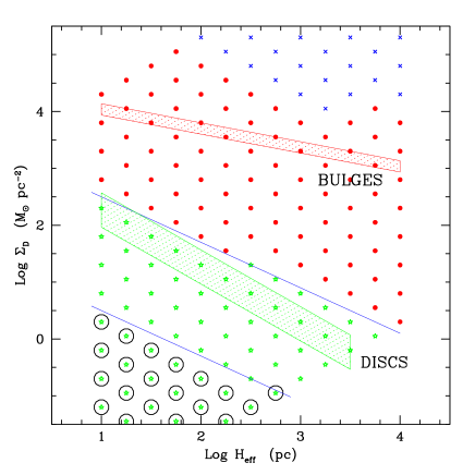
Figure 5: Feedback regimes as a function of surface mass density and vertical scale-length. Green stars denote systems in the adiabatic blow-out regimes (the encircled points highlight the unstable systems; see M04), red dots denote systems in the adiabatic confinement regime, blue crosses denote systems in the PDS confinement regime. The blue continuous lines separate the regions with different feedback regimes. The green and red shaded areas give the typical regions occupied by galaxy discs and bulges. This is an adapted version of figure 3a of M04.

In M04 it was shown that the dynamics of feedback depends mainly on the total surface density of the disc $\Sigma_{\rm D}$ and vertical scale-height $H_{\rm eff}$ of the system. In realistic systems feedback can take place in the regimes where super-bubbles blow-out or are confined in the adiabatic stage. Figure 5 shows that the adiabatic blow-out and confinement regimes take place in two different regions of the $\Sigma_{\rm D}$-$H_{\rm eff}$ space, separated by the relation:

$$\Sigma_{\rm D}=8\left(\frac{H_{\rm eff}}{1000\ {\rm pc}}\right)^{-0.8}\ \ {\rm M}_{\odot}\ {\rm pc}^{-2}$$ (51)

The numerical constants in this relation depend on the (uncertain) values of the parameters used in the model, so they are to be considered as indicative.

Galaxy discs and bulges tend to stay respectively in the adiabatic blow-out and confinement regimes, so at a basic level there is no much doubt on how to apply the feedback regimes within a galaxy formation code: discs are in the adiabatic blow-out regime, bulges are in the adiabatic confinement regime. However, the central region of a disc can be in the adiabatic confinement regime for at least two reasons: (i) it is embedded in a bulge, so that its ISM is pressurized by the bulge hot phase; (ii) its surface density is high enough to cross the limit of equation 51 for adiabatic confinement. This happens at a typical surface density of $\Sigma_{\rm D}\sim 100-300$ M_⊙ pc^-2. Point (i) has been used to justify the direct infall of gas from the halo to the bulge (section 5.4). Point (ii) has been mentioned in section 6.2 to argue for feedback-induced loss of angular momentum, and the effects of such feedback have been modeled by forcing bar formation when the surface density of cold gas is high (equation 50). We show more details and results on this mechanisms in Fontanot et al. (2006a).

To fully implement the M04 feedback recipes in morgana it is necessary to assess the role of the velocity dispersion of cold clouds, a quantity which is left as a free parameter in that paper. This is done in the following subsection. After that we explain how we implement feedback in the case of thin or thick systems.

7.1 Kinetic feedback and the velocity dispersion of cold clouds

We do not include here a full self-consistent treatment of the kinetic energy of cold clouds, but try to take into account its effect as follows. The velocity dispersion $\sigma_{\rm cold}=\sqrt{2K/M_{\rm cold}}$ of cold clouds in the ISM of a star-forming galaxy is determined as a first approximation (i.e. neglecting all mass flows) by the equilibrium between the injection of kinetic energy by SNe and the dissipation by turbulence:

$$\dot{K}=\dot{K}_{\rm SN}-\dot{K}_{\rm ds}$$ (52)

The injection of kinetic energy is:

$$\dot{K}_{\rm SN}=\epsilon_{k}\frac{\dot{M}_{\rm sf}}{M_{\rm\star,SN}}E_{\rm SN}$$ (53)

where $E_{\rm SN}$ is the energy of a SN, $M_{\rm\star,SN}$ is the mass of newly formed stars per SN and $\epsilon_{k}$ is its fraction given to the cold phase as kinetic energy. The rate of energy dissipation is observed in hydro simulation to be of the order (Mac Low 2003):

$$\dot{K}_{\rm ds}=\frac{1}{2}\frac{M_{\rm cold}\sigma_{\rm cold}^{3}}{L_{\rm drive}}$$ (54)

where $L_{\rm drive}$ is the scale at which turbulence is driven, suggested to be twice the diameter of the typical size of the super-bubble. To determine $\sigma_{\rm cold}$ we assume that an equilibrium configuration is quickly reached, so that $\dot{K}=0$. We then obtain:

$$\sigma_{\rm cold}=\sigma_{0}\,\left(\frac{t_{\star}}{1\ {\rm Gyr}}\right)^{-1/3}$$ (55)

where $\sigma_{0}=[2L_{\rm drive}\epsilon_{k}E_{\rm SN}/M_{\rm\star,SN}(1\ {\rm Gyr})]^{1/3}$ and the time-scale for star formation is $t_{\star}=M_{\rm cold}/\dot{M}_{\rm sf}$. In a thin system like the Milky Way the fraction of (thermal and kinetic) energy injected into the ISM is predicted by M04 to be about 5 per cent, so $\epsilon_{k}$ will be of order of 0.01, while the driving scale should be of order of the vertical scale-length of the system, $\sim 100$ pc. The numerical value of $\sigma_{0}$ is then:

$$\sigma_{0}=9.3\left(\frac{L_{\rm drive}}{100\ {\rm pc}}\right)^{1/3}$$

$$\times\left(\frac{\epsilon_{k}}{0.01}\right)^{1/3}E_{51}^{1/3}\left(\frac{M_{\rm\star,SN}}{120\ {\rm M}_{\odot}}\right)^{-1/3}\ {\rm km\ s}^{-1}$$

The predicted value of $\sigma_{\rm cold}$ for a Milky Way-like galaxy (with $t_{\star}\sim 2$ Gyr) is then $\sim 7$ km s^-1, in remarkable agreement with the observed value which ranges between 6 and 9 km s^-1. Much higher values of the velocity dispersion are expected in thick systems, where $\epsilon_{k}$ is much higher (all the SN energy is retained by the system) and $t_{\star}$ much lower. This is in agreement with the sparse data available (see, e.g., Dib, Bell & Burkert 2006 for local galaxies, and Genzel et al. 2006 for galaxies at $z\sim 2$). As a consequence, we neglect kinetic feedback in discs but take it into account in bulges. Given the great uncertainty in the driving scale of turbulence in mergers, the normalization constant $\sigma_{0}$ will be left as a free parameter.

We stress that equation 7.1 is valid under the assumption that turbulence is driven by SNe and not by gravitationally induced motions like differential rotation or tidal disturbances in mergers. In the case of our Galaxy, Mac Low (2003) argues from energetic arguments that SNe are the most likely drivers of turbulence, and the good agreement of the predicted value of $\sigma_{\rm cold}$ given above with the observed one suggests that they are at least a significant contributor. In thick systems, like gas-rich spheroids or mergers, gravitationally-induced turbulence will be very important. However, the most relevant consequence of a high value of $\sigma_{\rm cold}$ for our purposes is the massive removal of cold gas during episodes of strong star formation. It is clear that if a condition $\sigma_{\rm cold}>V_{\rm B}$ is reached in a gas-rich bulge, then the driver of turbulence must be star formation and not gravity, while in the case of a low value of $\sigma_{\rm cold}$ no mass is removed. So, in this case the assumption will work in the range where its results are most influential.

7.2 Discs as thin systems

In thin systems, super-bubbles blow out of the disc soon after they form and while they are still in the adiabatic stage; their porosity remains low. The fraction of the SN energy that is injected into the ISM is limited to a few per cent of the total budget, while most energy is directly injected into the halo through a tenuous, metal-rich hot wind. The ISM self-regulates to a configuration that is very similar to that of the Milky Way (M04). The star formation regulates to a level similar to that found in nearby galaxies by Schmidt (1959) and quantified more recently by Kennicutt (1998).

In M04 the resulting star-formation timescales were incorrectly scaled with the infall time and the total surface density $\Sigma_{\rm D}$ of the system. A more careful analysis reveals that, for a fixed set of parameters and at fixed $H_{\rm eff}$, $t_{\star}$ depends mostly on the cold gas surface density $\Sigma_{\rm cold,D}$. This is expected, as the star-formation timescale is determined by the intrinsic properties of the ISM, not by the rate at which mass is acquired by it or by the amount of stars present. A better fit of the results of M04 in the adiabatic blow-out regime (for the standard set of parameters defined in that paper) gives:

$$t_{\star}=6\,\left(\frac{\Sigma_{\rm cold,D}}{1\ {\rm M}_{\odot}\ {\rm pc}^{-2}}\right)^{-0.4}\left(\frac{H_{\rm eff}}{100\ {\rm pc}}\right)^{0.65}\ {\rm Gyr}$$ (57)

In the simple case of a constant value of $H_{\rm eff}$ for all galaxies, the Schmidt-Kennicutt law is recovered with a very similar normalization (however, observations refer to integrated quantities, this prediction refers to a section of the disc). But the assumption of a constant $H_{\rm eff}$ is rather artificial, as the vertical scale-length of the cold gas is determined by the vertical gravitational equilibrium as $H_{\rm eff}=\sigma_{\rm cold,D}^{2}/\pi G\Sigma_{\rm D}$, so a constant value would imply a tuned variation of $\Sigma_{\rm D}$ and $\sigma_{\rm cold,D}$. The other simple possibility is to assume a constant value for $\sigma_{\rm cold,D}$. This leads to the prediction $t_{\star}\propto\Sigma_{\rm cold,D}^{-1.05}f_{\rm cold}^{0.65}$, where $f_{\rm cold,D}$ is the fraction of cold gas in the disc. This relation is apparently steeper than the observed Schmidt law; however, $\Sigma_{\rm cold,D}$ and $f_{\rm cold,D}$ are usually correlated in galaxies, in that lower $\Sigma_{\rm cold,D}$ discs, having lower star-formation rates, retain a greater fraction of their gas. For instance, with our reference choice of parameters (section 12) we obtain $f_{\rm cold,D}\propto\Sigma_{\rm cold,D}^{0.8}$, which implies the much shallower relation $t_{\star}\propto\Sigma_{\rm cold,D}^{-0.53}$.

The dependence of the velocity dispersion on the star-formation timescale, equation 55, is then inserted, through the definition of $H_{\rm eff}$, into equation 57, and the resulting relation is normalized so as to lie on the average Schmidt-Kennicutt relation at $\Sigma_{\rm cold,D}=13$ M_⊙ pc^-2(the gas density of the Milky Way, obtained by assuming $R_{\rm D}=3.5$ kpc and $M_{\rm cold,D}=5\times 10^{9}$ M_⊙, see Cox 2000). The resulting relation for the star-formation timescale in discs is:

$$t_{\rm\star,D}=9.1\;\left(\frac{\Sigma_{\rm cold,D}}{1\ {\rm M}_{\odot}\ {\rm pc}^{-2}}\right)^{-0.73}\left(\frac{f_{\rm cold,D}}{0.1}\right)^{0.45}\ {\rm Gyr}$$ (58)

This relation is again apparently steeper than the Schmidt-Kennicutt one, but when the correlation between $\Sigma_{\rm cold,D}$ and $f_{\rm cold}$ is taken into account we obtain $t_{\rm\star,D}\propto\Sigma_{\rm cold,D}^{-0.37}$ or $\Sigma_{\rm sfr,D}\propto\Sigma_{\rm cold,D}^{1.37}$, in excellent agreement with the observed Schmidt law.

Other complications can be introduced in this picture: if the driving length $L_{\rm drive}$ is equal to twice the diameter of the blowing-out super-bubbles, it will scale with $H_{\rm eff}$. Moreover, the efficiency of feedback is known in M04 to increase slightly with $\Sigma_{\rm D}$ (and then with $\Sigma_{\rm cold,D}$). Introducing these dependences we obtain a scaling of $t_{\star}$ with $\Sigma_{\rm cold,D}$ and $f_{\rm cold,D}$ similar to equation 58, with slightly different exponents. We have verified that these somewhat different descriptions of feedback do not give significantly different results, so we keep equation 58 as a reference.

According to M04, in the adiabatic blow-out regime the mass ejection rate due to the action of super-bubbles is modest, while much gas belonging to the hot phase leaks out of the halo simply because it is too hot to be confined by the disc. This unavoidable mass flow, observed as a hot corona surrounding the star-forming discs (see, e.g., Fraternali et al. 2002), amounts to a mass ejection rate very similar to the star-formation rate. We then set the disc hot wind term $\dot{M}_{\rm hw,D}$ as equal to the star formation rate $\dot{M}_{\rm sf,D}$. This is at variance with most other galaxy formation models, where the rate of gas re-heating, equivalent to our $\dot{M}_{\rm hw,D}$, is related to the star-formation rate through a $\beta$ parameter, assumed to scale as a power of the disc velocity. Our assumption is equivalent to $\beta=1$; the higher ejection efficiency in small discs will then be due to galaxy super-winds triggered by the energy injection from the galaxy. Finally, we neglect any cold wind term, due to the results of M04 and to the predicted low level of turbulence in discs (section 7.1).

Using the instantaneous recycling approximation (see also section 8), we let a fraction $f_{\rm rest}$ of the mass of newly formed stars to be restored to the ISM. Summing up, the star-formation, restoration and wind mass flows in discs are:

$$\begin{array}[]{lll}\dot{M}_{\rm sf,D}&=&\dot{M}_{\rm cold,D}/t_{\rm\star,D}\\ \dot{M}_{\rm rs,D}&=&f_{\rm rest}\dot{M}_{\rm sf,D}\\ \dot{M}_{\rm hw,D}&=&\dot{M}_{\rm sf,D}\\ \dot{M}_{\rm cw,D}&=&0\end{array}$$ (59)

The hot wind mass flow does not carry much thermal energy: assuming a typical temperature of $10^{6}$ K (M04) and for $M_{\rm\star,SN}=120$ M_⊙ and $10^{51}$ erg per SN, the fraction of SN energy carried away by this wind is $\simeq 0.05$. However, most SN energy is blown out to the halo by the blowing-out super-bubbles, and this energy mixes with the thermal energy of the hot outflowing wind. We then assume that a fraction $f_{\rm th,D}$ of a $10^{51}$ erg SN is carried by the hot wind gas; this fraction is estimated to be $\sim 0.8$ by Monaco (2004b). However, this number is highly uncertain because (i) the loss of SN energy within the star-forming cloud could be higher, as many authors working on the physics of ISM have often claimed, (ii) the SN energy could be well in excess of $10^{51}$ erg, (iii) some energy could be lost in the interaction with the hot halo gas. Moreover, there is a degeneracy between this parameter and $M_{\rm\star,SN}$, which depends on the IMF. It is then wise to leave $f_{\rm th,D}$ as a free parameter; it is however remarkable that its best-fit value turns out to be 0.5, not far from the value suggested by Monaco (2004b).

To the energy of type II SNe we add a contribution from type Ia SNe as one per year per $10^{12}$ M_⊙ of stars. This is done in order to test the energetic effect of these SNe. In the case of thin systems with a continuous star formation, and given the uncertainty on $f_{\rm th,D}$, the contribution from type Ia SNe is almost irrelevant. As suggested for instance by Recchi et al. (2002), type Ia SNe may have a higher efficiency of energy injection, as they don’t explode in the dense molecular clouds. As a consequence, one might want to have a different efficiency $f_{\rm th,Ia}$ for the two SN types. However, given the modest importance of these objects we prefer not to add a further parameter.

The contribution of the disc to the hot wind energy term is then:

$$\left.\dot{E}_{\rm hw,H}\right|_{\rm disc}=f_{\rm th,D}E_{\rm SN}\left(\frac{\dot{M}_{\rm sf,D}}{M_{\rm\star,SN}}+1\ {\rm SN\ yr}^{-1}\frac{M_{\rm star,D}}{10^{12}\ {\rm M}_{\odot}}\right)$$ (60)

The outflowing hot gas will interact with the halo cold phase in a way that is difficult to model. In order to be able to constrain the effect of this process, we allow for a fraction of the thermal energy to be given to the halo cold phase:

$$\left.\dot{K}_{\rm w,H}\right|_{\rm disc}=f_{\rm kin}\left.\dot{E}_{\rm hw,H}\right|_{\rm disc}$$ (61)

For simplicity we do not subtract this energy from the hot wind budget. We stress that this term is not due to a contribution of cold wind but to the interaction of the hot wind with the cold halo phase.

Star formation in the external parts of galaxy discs is known to be truncated (see, e.g., Kennicutt 1989), and this is likely due to the differential rotation, even though also the thermal transition from warm to cold gas may play a crucial role, as suggested by Shaye (2004). This author also suggests that the threshold for star formation may be simply expressed in terms of a threshold for gas surface density, which scales with the disc and ISM properties and, very importantly, with the ionizing UV background. We implement this threshold $\Sigma_{\rm thr}$ for star formation simply by increasing the star-formation timescale $t_{\rm\star,D}$ by the inverse of the fraction of disc mass for which $\Sigma_{\rm cold,D}>\Sigma_{\rm thr}$. Clearly, a better but more complicated choice would be to divide the disc into three zones, corresponding to the bulge, the star-forming disc and the gas beyond the star-formation threshold; this is left to future work. We have also tried to modulate this threshold with redshift, following the increase by an order of magnitude of the ionizing background from $z=0$ to 1 (Bianchi, Cristiani & Kim 2001). However, the dependence of the threshold on the ionizing background, is so weak that this modulation does not influence the results appreciably.

7.3 Bulges as thick systems

In the model by M04 the gravitational perturbations to the ISM are neglected. This assumption is questionable for spiral discs, but the coincidental similarity between the timescale for kinetic aggregations and the disc timescale, that drives the sweeping by spiral arms, makes the kinetic aggregation mechanism a good substitute for spiral arms in creating massive clouds, at least at an order-of-magnitude level. Things change in the case of thick systems like bulges, where most energy is efficiently pumped into the hot phase so that the ISM is much more pressurized, the star-forming clouds are much smaller and denser, and kinetic aggregations are disfavored. This leads to the prediction of a lower level of star formation compared with the Schmidt-Kennicutt law (figure 7 of M04). However, tidal disturbances will be much stronger in a bulgy object, at least when it is formed through a disc instability or a merger, so that the formation of collapsing clouds will not be determined by kinetic aggregations. Moreover, in a major merger the pressurization due to the onset of the adiabatic confinement regime will cause a quick drop of the Jeans mass, and this will make most clouds present in the merging discs collapse and form stars in a short time. These transient effects have not been properly modeled by M04, so we prefer to determine the star-formation timescale directly from the Schmidt law:

$$t_{\rm\star,B}=4\;\left(\frac{\Sigma_{\rm cold,B}}{1\ {\rm M}_{\odot}\ {\rm pc}^{-2}}\right)^{-0.4}\ {\rm Gyr}$$ (62)

The resulting star-formation and restoration rates in bulges are:

$$\begin{array}[]{lll}\dot{M}_{\rm sf,B}&=&M_{\rm c,B}/t_{\rm\star,B}\\ \dot{M}_{\rm rs,B}&=&f_{\rm rest}\dot{M}_{\rm sf,B}\end{array}$$ (63)

As for the thin system case, the rate at which hot gas flows to the halo is similar to the star formation rate, so that we retain this prediction. While in thin systems most energy (though not most mass) is injected to the halo mainly by blowing-out super-bubbles, in thick systems the energy is ejected mainly through this hot wind. In the M04 model the typical temperature of the hot phase is found to be of $\sim 10^{7}$ K, higher by an order of magnitude than the thin system case; the fraction of SN energy carried away by the hot wind is then $f_{\rm th,B}\simeq 0.5$, slightly lower than the thin system case. Moreover, while a disc is unable to confine a gas phase with a temperature as high as $\sim 10^{6}$ K, a massive bulge can gravitationally confine its hot phase, whose temperature corresponds roughly to the virial temperature of a bulge with $V_{\rm B}\sim V_{\rm hot}=300$ km s^-1. We then limit the hot wind as follows:

$$\beta=\frac{\sqrt{V_{\rm hot}^{2}-V_{\rm B}^{2}}}{V_{\rm hot}}$$ (64)

where of course $\beta=0$ if $V_{\rm B}>V_{\rm hot}$. The resulting hot wind rate is:

$$\left.\dot{M}_{\rm hw,B}\right|_{\rm therm}=\beta\dot{M}_{\rm sf,B}$$ (65)

while the hot wind energy is:

$$\left.\dot{E}_{\rm hw,H}\right|_{\rm bulge}$$

$$= f_{\rm th,B}E_{\rm SN}\beta\left(\frac{\dot{M}_{\rm sf,B}}{M_{\rm\star,SN}}+1\ {\rm SN\ yr}^{-1}\frac{M_{\rm star,B}}{10^{12}\ {\rm M}_{\odot}}\right)$$

As for the thin systems, we allow some energy to accelerate the cold halo phase:

$$\left.\dot{K}_{\rm w,H}\right|_{\rm bulge,hw}=f_{\rm kin}\left.\dot{E}_{\rm hw,H}\right|_{\rm bulge}$$ (67)

Because in thick systems all the energy of SNe is injected to the ISM and star-formation timescales are much shorter (in virtue of the increased surface density), the injection of kinetic energy leads to velocity dispersions of the cold phase much larger than the $\sim$7 km s^-1 found in discs. In this case some cold clouds may get enough kinetic energy to be able to leave the potential well of the bulge. The probability that a cold cloud is unbound, i.e. it has a velocity larger than the escape velocity of the bulge, $\sqrt{2}V_{\rm B}$, is computed under the hypothesis of a Maxwellian distribution of velocities with rms $\sigma_{\rm cold,B}$:

$$P_{\rm unb}={\rm erfc}\left(\frac{V_{\rm B}}{\sigma_{\rm cold,B}}\right)+\frac{2}{\sqrt{\pi}}\frac{V_{\rm B}}{\sigma_{\rm cold,B}}\exp\left(-\frac{V_{\rm B}^{2}}{\sigma_{\rm cold,B}^{2}}\right)$$ (68)

The average velocity of the unbound clouds is:

$$v_{\rm unb}=\sigma_{\rm cold,B}\frac{4}{\sqrt{2\pi}}\frac{\left(1+\left(\frac{V_{\rm B}}{\sigma_{\rm cold,B}}\right)^{2}\right)\exp\left(-\frac{V_{\rm B}^{2}}{\sigma_{\rm cold,B}^{2}}\right)}{P_{\rm unb}}$$ (69)

The velocity of the clouds after being ejected out of the bulge will be:

$$v_{\rm out}=\sqrt{v_{\rm unb}^{2}-2V_{\rm B}^{2}}$$ (70)

This process will generate a wind flux roughly equal to the unbound mass, $P_{\rm unb}M_{\rm c,B}$, divided by the crossing time $R_{\rm B}/v_{\rm unb}$. This outflow is naturally identified with a cold wind, adding mass to the cold halo phase. The cold wind mass flow is:

$$\dot{M}_{\rm cw,B} = M_{\rm c,B}P_{\rm unb}\frac{v_{\rm unb}}{R_{\rm B}}$$ (71)

$$\left.\dot{K}_{\rm w,H}\right|_{\rm bulge,cw} = \frac{1}{2}\dot{M}_{\rm cw,B}v_{\rm out}^{2}$$ (72)

However, the fate of the cold clouds ejected by a bulge may be different. The exit from the pressurized bulge to the halo would lead to an expansion of those clouds, making them much more sensitive to the bow shock generated in their interaction with the hot halo gas and to thermal evaporation. As a result, the cold clouds ejected by the bulge could be heated and mix with the hot phase. This is analogous (though not in the details) to what happens when kinetic feedback is implemented in SPH simulations: a cold particle neighbouring a star-forming region is given some kinetic energy, but this energy is quickly thermalized by the interaction with the other particles. If this is the case, the cold and hot wind flows should be given as follows:

$$\left.\dot{M}_{\rm hw,B}\right|_{\rm kin} = M_{\rm c,B}P_{\rm unb}\frac{v_{\rm unb}}{R_{\rm B}}$$ (73)

$$\dot{M}_{\rm hw,B} = \left.\dot{M}_{\rm hw,B}\right|_{\rm therm}+\left.\dot{M}_{\rm hw,B}\right|_{\rm kin}$$ (74)

$$\dot{M}_{\rm cw,B} = 0$$ (75)

From the energetic point of view, the kinetic energy of this outflow will be typically not enough to heat the gas to a high temperature, so the heating will be done with the same energy budget of equation 7.3; in other words, no energy is added to the $\dot{E}_{\rm hw,H}$ term. We have implemented both possibilities, and the choice between the two has been left free. The results presented here are obtained giving the outflowing gas to the hot phase.

8 Metals

The evolution of metals is given by the equations reported in table 1. In this set of equations most metal flows are obtained from their related mass flow as follows:

$$\dot{M}^{Z}_{\rm flow}=\frac{M^{Z}_{\rm source}}{M_{\rm source}}\dot{M}_{\rm flow}$$ (76)

where $M_{\rm source}$ and $M^{Z}_{\rm source}$ are the gas and metal masses of the source phase. The cosmological infalling gas is assumed to have a metallicity $Z_{\rm pre}\sim 10^{-6}$ due to pre-enrichment by sources that are below the mass resolution limit (from popIII stars to very small primeval galaxies). These flows take into account the transfer of metals among phases and components, but not their production.

We assume that (i) metals are produced by newly formed stars in the instantaneous recycling approximation, i.e. their production follows instantaneously star formation; (ii) the new metals are instantaneously mixed with the ISM. Newly metals are spread into the ISM mainly by SNe, so analogously to the energy they are likely to be selectively ejected to the halo. This is clearly true in the blowing-out thin systems, but even in thick systems metals are first mixed with the hot gas that escapes the halo at a rate equal to the star-formation rate. To model this effect without using explicitly a multi-phase description of the ISM, a fraction $f_{\rm Zej}$ of the new metals is ejected directly to the halo through hot winds. In the case of bulges, this fraction is multiplied by the $\beta$ factor of equation 64, to take into account the ability of massive bulges to retain the outflowing hot gas. We have:

$$\left.\dot{M}^{Z}_{\rm hw,H}\right|_{\rm ej}=f_{\rm Zej}Y\left(\beta\dot{M}_{\rm sf,B}+\dot{M}_{\rm sf,D}\right)$$ (77)

where $Y$ is the fraction of mass in newly produced metals per generation of stars. This term is added to the $\dot{M}^{Z}_{\rm hw,H}$ metal flow; satellite galaxies will inject their metals to the halo component of the main DM halo they belong to through the satellite metal flows. The other metals will be given to the ISM of the component they belong to:

$$\dot{M}^{Z}_{\rm yi,B} = (1-\beta f_{\rm Zej})Y\dot{M}_{\rm sf,B}\,,$$

$$\dot{M}^{Z}_{\rm yi,D} = (1-f_{\rm Zej})Y\dot{M}_{\rm sf,D}\,,$$ (78)

A value of $f_{\rm Zej}=0.5$ will be used in the following.

9 AGN activity

9.1 Accretion onto black holes

The modeling of black hole accretion in morgana has already been described, though in a slightly different way, by Monaco & Fontanot (2005), and will be briefly summarized here.

A seed black hole of mass $M_{\rm seed}$ is put at the centre of each DM halo. These black holes may be generated by the collapse of the first stars (e.g., Volonteri, Haardt & Madau 2003). Seed masses should be of order of tens to hundreds M_⊙; however, they start growing very soon during the early evolution of baryons in DM halos. This happens at times and for DM halo masses that are not sampled in the typical runs used in galaxy formation. We then use a higher value for the seed mass, $M_{\rm seed}=1000$ M_⊙; the results are quite stable for reasonable variations of this parameter.

The accretion of gas onto the black holes is possible only if this gas has lost nearly all of its angular momentum. The first step in this loss is the same that leads to the formation of bulges; we then base our computation of black hole accretion on the cold bulge gas. As the amount of accreted gas is small, we do not remove the accreted mass from the matter budget. In other words, the mass in black holes does not obey a mass conservation constraint as the mass of all the other components.

The gas is assumed to lose angular momentum at a rate proportional to the star-formation rate. This is justified by the radiation drag mechanism proposed by Umemura (2001) and used by Granato et al. (2004). However, a connection between loss of angular momentum and star formation likely has a more general validity, as many mechanisms able to cause a loss of angular momentum (turbulence, kinetic aggregations etc.) are directly or indirectly driven by massive stars and SNe. The simplest way of modeling the loss of angular momentum is then:

$$\dot{M}_{\rm lowJ}=f_{\rm lowJ}\dot{M}_{\rm sf,B}$$ (79)

More generally, the accreted mass could scale as a power law of the star-formation rate; for instance, angular momentum loss driven by encounters would likely scale with the square of the driving force. This is described in detail in Fontanot et al. (2006a); we describe here only the simplest choice.

We follow Granato et al. (2004) by assuming that this gas does not flow directly onto the black hole but settles on a reservoir of low-angular momentum gas, whose mass is $M_{\rm resv}$. From this reservoir the gas accretes onto the black hole at a rate regulated by the viscous time-scale of the accretion disc, modeled by Granato et al. (2004) as:

$$\dot{M}_{\rm visc}=k_{\rm accr}\frac{\sigma_{\rm B}^{3}}{G}\left(\frac{M_{\rm res}}{M_{\rm BH}}\right)^{3/2}\left(1+\frac{M_{\rm BH}}{M_{\rm resv}}\right)^{1/2}$$ (80)

where the constant $k_{\rm accr}$ is suggested by the authors to take a value $\sim$0.001, $\sigma_{\rm B}\simeq 0.65V_{\rm B}$ is the 1D velocity dispersion of the bulge and $M_{\rm BH}$ is of course the BH mass.

Accretion is always limited by the Eddington-Salpeter rate, whose time-scale (for a radiation efficiency of 0.1) is $t_{\rm Ed}=0.04$ Gyr. The evolution of the black hole-reservoir system is then:

$$\begin{array}[]{lll}\dot{M}_{\rm BH}&=&\min\left(\dot{M}_{\rm visc}\,,\,\frac{M_{\rm BH}}{t_{\rm Ed}}\right)\\ \dot{M}_{\rm resv}&=&\dot{M}_{\rm lowJ}-\dot{M}_{\rm BH}\end{array}$$ (81)

In Monaco & Fontanot (2005), the accretion rate onto the black hole was modeled simply as $M_{\rm resv}/t_{\rm Ed}$. We prefer equation 80 in virtue of its sounder physical motivation.

9.2 Feedback from jets

Jets coming from radio-loud AGNs are though to be one of the most promising mechanisms to stop the cooling flows in galaxy clusters (McNamara et al. 2005; Voit & Donahue 2005). Besides, a successful reproduction of the high-luminosity cutoff of the luminosity function of galaxies requires a proper modeling of this kind of feedback (Benson et al. 2003; Bower et al. 2006; Croton et al. 2006). The efficiency of radiation of AGNs is known to decrease when the accretion rate in units of the Eddington rate $\dot{m}=\dot{M}_{\rm BH}t_{\rm Ed}/M_{\rm BH}$ is lower than $\sim 10^{-2}$; these slowly accreting black holes however radiate very efficiently in the radio (see the discussion in Merloni, Heinz & Di Matteo 2003). It is then reasonable to assume that the efficiency of energy emission in jets is 0.1 if $\dot{m}$ is small, and lower for higher accretion rates. As $\sim$10 per cent of bright QSOs are radio-loud, we estimate the efficiency of jet emission as 0.01 in the case of $\dot{m}>0.01$.

As suggested by Croton et al. (2006), the efficiency with which this energy heats the hot halo gas component should scale with the hot gas temperature to the power 3/2. In order to keep the expression simple and avoid possible unwanted numerical instabilities in the integration, we scale the efficiency with the circular velocity of the halo:

$$f_{\rm jet}=f_{\rm jet,0}\left(\frac{V_{c}}{1000\,{\rm km\ s}^{-1}}\right)^{3}$$ (82)

The energy injected into the halo hot gas is then:

$$\left.\dot{E}_{\rm hw,H}\right|_{\rm jets}=\left\{\begin{array}[]{lll}f_{\rm jet}0.1\,\dot{M}_{\rm BH}c^{2}&{\rm if}&\dot{m}<0.01\\ f_{\rm jet}0.01\,\dot{M}_{\rm BH}c^{2}&{\rm if}&\dot{m}>0.01\end{array}\right.$$ (83)

This mechanism benefits much by the direct infall of gas to the bulge, described in section 6.2, but, as demonstrated in appendix B, works only for particle masses not higher than $10^{9}$ M_⊙.

9.3 Quasar-triggered galaxy winds

A bright quasar shining into a star-forming bulge can inject a great amount of energy into the ISM, leading to a massive removal of cold gas. This mechanism has been described in detail by Monaco & Fontanot (2005). These winds have a modest effect on the formation of a galaxy, but influence the formation and evolution of AGNs. This is described in full detail in Fontanot et al. (2006a), where models with quasar-triggered winds are presented. We do not use these winds in the results presented in this paper, as the introduction of winds influences deeply the number of bright quasars but only modestly their host galaxies.

10 Parameters

	Name	reference	Comment	Constraint	Equation/
		model			Section
			mergers
	$f_{\rm hmm}$	0.2	major merger condition for DM halos	N-body	eq. 10
	$f_{\rm gmm}$	0.3	major merger condition for galaxies	N-body	eq. 11
	$f/c$	2.0/4.0	bulge formation in mergers/disc instabilities	N-body	eq. 49
!	$f_{\rm scatter}$	0.1	fraction of stars scattered at a galaxy major merger	N-body	sect.4.3
			halo component
!	$\gamma_{p}$	1.15	polytropic index of the hot gas	observ.	eq. 13
	$f_{\rm shock}$	1.2	shock heating factor	N-body	eqs. 20, 21
!	heat cold gas	YES	switch for heating cold halo gas at major mergers	N-body	sect. 5.2
!	$n_{\rm quench}$	1.0	no. of crossing times for quenching cooling	free	sect. 5.2
!	close hole	YES	switch for closing the cooling hole	free	eq. 29
!	infall on bulge	YES	switch for allowing infall on the bulge	free	eqs. 33, 35
!	$n_{\rm dyn}$	1.0	no. of dynamical times for infall	free	eqs. 31, 32
!	$f_{\rm wind}$	1.7	energy factor to trigger a super-wind	free	eqs. 37, 41
	$f_{\rm back}$	0.5	fraction of super-wind mass that falls back	free	sect. 5.5
			disc structure
	$\epsilon_{\rm limit}$	0.9	limit for bar instability	N-body	eq. 48
	$f_{\rm bar}$	0.5	fraction of disc that goes to bulge	free	sect. 6.2
	adiabatic contr.	NO	switch for adiabatic contraction	free	eq. 47
			stars and metals
	$M_{\rm\star,SN}$	120 M⊙	stellar mass per SN	IMF	eqs. 60, 7.3
	$f_{\rm rest}$	0.4	fraction of restored mass	IMF	eqs. 59, 63
!	$Y$	0.03	metal yield per generation	observ.	eqs. 77, 78
	$Z_{\rm pre}$	$10^{-6}$	metallicity due to pre-enrichment	free	sect. 8
!	$f_{\rm Zej}$	0.5	fraction of metals ejected to halo	free	eqs. 77, 78
			star formation and feedback
!	$f_{\rm th,D}$	0.5	thermal efficiency of feedback in thin systems	free	eq. 60
!	$f_{\rm th,B}$	0.5	thermal efficiency of feedback in thick systems	free	eq. 7.3
!	$f_{\rm kin}$	0	kinetic energy from hot winds	free	eqs. 61, 67
!	$\sigma_{0}$	60 km s-1	turbulent velocity of clouds	free	eqs. 55, 7.1
!	$\Sigma_{\rm thr}$	0 M⊙ pc-2	gas surface density threshold for star formation	observ.	section 7.2
!	$\Sigma_{\rm limit}$	$\infty$ M⊙ pc-2	critical gas surface density for discs	free	eq. 50
!	hot kin. fb	YES	switch for heating cold gas by kinetic feedback	free	eqs. 71-75
			AGN
	$M_{\rm seed}$	1000 M⊙	seed black hole mass	theory	sect. 9.1
!	$f_{\rm lowJ}$	0.003	rate of loss of angular momentum	free	eq. 79
!	$f_{\rm jet,0}$	1	efficiency of jet feedback for a 1000 km s-1 halo	N-body	eq. 82
			numerical parameters
!	$M_{\rm part}$	$10^{9}$M⊙	particle mass	—	—
	$\Delta_{t}$	0.1 Gyr	numerical interval for the integration	free	sect. 2.2

Table 4: Model parameters, with their value adopted in the reference model, brief description, available constraints (independently of the model) and reference in the text. Parameters highlighted by a mark are of primary importance. Cosmological parameters are not included.

Table 4 gives a complete list of the parameters of the model, with the value used to compute the results given in this paper. To these the cosmological parameters ($\Omega_{0}$, $\Omega_{\Lambda}$, $\Omega_{b}$, $H_{0}$ and $\sigma_{8}$; see the Introduction) should be added; these are now fixed with a good accuracy, with the exception of $\sigma_{8}$ whose value influences strongly the number of galactic DM halos at high redshift. The number of parameters is high, and this reflects both the number of physical processes that are included in the galaxy formation code and the level of uncertainty in many of these processes. Anyway, galaxy formation is a problem of complexity, and there is no way to reduce the number of parameters other than hiding them by fixing them to some value. On the other hand, the number of observables that can be used to constrain these parameters is very high, so their values can be fixed, with the exception of a few degeneracies. The most obvious one in this context is the degeneracy between the energy of a SN, the star mass per SN $M_{\rm star,SN}$ and the thermal feedback efficiencies $f_{\rm th,B}$ and $f_{\rm th,D}$ (equations 60 and 7.3). For this reason we only vary the efficiencies, leaving $M_{\rm\star,SN}$ fixed and not even including the SN energy as a parameter.

In practice, many of these parameters are fixed independently by the results of N-body simulations (like the parameters of merging) or by the knowledge of the IMF, and their variation within the known uncertainties does not influence the results strongly. The remaining parameters, labeled with a mark in the table, are then of primary importance. Their value is fixed by comparing with a set of basic data (section 12), we give here a very brief list of the observable which is most useful to fix each parameter.

$f_{\rm scatter}$: it regulates the amount of halo stars, and is fixed by requiring a fraction of at least $\sim 20$ per cent of halo stars in groups and clusters ($M_{\rm H}\ga 10^{14}$ M_⊙).

$n_{\rm quench}$ and $n_{\rm dyn}$: they regulate the star formation density, especially at high redshift; their value is fixed by reproducing the very uncertain star formation density at $z>4$. They are nearly degenerate and their value is especially sensitive to mass resolution.

$\gamma_{p}$: it regulates star formation, especially at low redshift, but its influence is modest when it is varied within the range suggested by observations.

$f_{\rm wind}$: by regulating the energy level at which a galactic super-wind is triggered, it influences the relation between stellar and DM mass.

heat cold gas: its switching on gives an effect similar to an increase of $n_{\rm quench}$ or $n_{\rm dyn}$ by 1.

close hole: when it is on, it increases cooling by a significant amount which depends on $\gamma_{p}$. All the parameters of the hot halo gas and stellar feedback should be re-tuned if this option is active.

infall on bulge: it influences mostly the jet feedback, so it should be switched on if an efficient quenching of the cooling flow is wanted.

$Y$: it regulates the amount of metals produced by stars, and is fixed by requiring a good match of galaxy metallicities.

$f_{\rm Zej}$: it regulates the fraction of metals injected in the halo component, and is fixed by requiring a good match of the metal enrichment of the hot halo gas.

$f_{\rm th,D}$: it regulates the stellar mass of small galaxies, and is fixed by requiring a good match of the power-law part of the stellar mass function.

$f_{\rm th,B}$, $f_{\rm kin}$ and hot kin. fb: they have only a modest influence on the results, so they are left to their reference values.

$\sigma_{0}$: it influences star formation in small bulges, and then the amount of downsizing of the AGN population; it is fixed as explained in Fontanot et al. (2006a).

$\Sigma_{\rm thr}$: it influences the mass of cold gas in local discs and its value is suggested by observations.

$\Sigma_{\rm limit}$: it influences the history of star formation and BH accretion in a rather subtle way; it is used in Fontanot et al. (2006a).

$f_{\rm lowJ}$: it regulates the BH–bulge relation at $z=0$, and its value depends on whether quasar-triggered winds are switched on; see Fontanot et al. (2006a) for details.

$f_{\rm jet,0}$: its value is suggested to be unity by N-body simulations, and it allows to quench cooling flows and limit the mass of elliptical galaxies.

11 Post Processing

For each tree that is analyzed, all the variables introduced in section 2.3, together with the disc and bulge radii and velocities, star formation rates and accretion rate onto black holes (at the sampling time, not averaged over the time bin), are sampled in intervals of time $\Delta_{t}$ and at the final time. All these quantities are output at the end, together with the merger histories of galaxies, constructed as specified in section 3.1.

For each time bin this information is issued for all the existing galaxies of a tree. However, this is not sufficient to reconstruct the star-formation history of a galaxy component, because disc instabilities, mergers, tidal stripping and destruction events move stars among galaxies and components; as a consequence, the sampled star formation history of stars that are formed in a galaxy component does not coincide with the star formation history of the stars eventually found in that galaxy component. To reconstruct this last quantity, all the events that transfer stellar mass from a component or a galaxy to another are recorded and output at the end. Star formation histories are then reconstructed at the post-processing stage by scrolling the sampled history of galaxies and moving stellar mass among the components. This is a very quick process, that can be done at the reading time.

The output of morgana (star formation histories and metallicities of the cold gas) is then given to the spectro-photometric code grasil (Silva et al. 1998), which is able to predict the SEDs of the predicted galaxies from the UV to the radio. This way it is possible to construct predictions for the luminosity functions at a fixed redshift or in redshift intervals, galaxy number counts and galaxy backgrounds. The grasil code has been tested against many local and distant galaxies and is widely used by the community; however, it introduces further uncertainties and parameters, so we prefer in this paper to discuss only the prediction of morgana before its interfacing with grasil. All the details of this interfacing will be given in Fontanot et al. (2006b).

The star formation rates are then reconstructed in time bins of width $\Delta_{t}$, which is set to 0.1 Gyr. This sampling is fine but for the last bin considered, as the last formed stars, that dominate the UV, B and FIR spectra, live for less than the sampling bin. To overcome this difficulty, we sample also the value of bulge and disc star-formation rates evaluated at the end of each time bin. Then, for each galaxy component, the time bin corresponding to the time at which the SED is computed is split into two parts, of widths 0.09 and 0.01 Gyr. To the second part we assign a star-formation rate equal to the punctual value at the end of the bin, while to the first part we assign a star-formation rate such as the integral over the bin gives the total amount of stars. As grasil re-samples the star-formation histories on a much finer time grid, this procedure is accurate as long as the star formation rate does not vary strongly on timescales smaller than 10 Myr, which is the case for most galaxies. The accuracy of this procedure with respect to the use of the complete star-formation rate produced by morgana during the integration will be shown in Fontanot et al. (2006b).

To compute the AGN activity of galaxies, a sampling in a time grid is not sufficient, due to the low duty cycle of AGNs. To optimize the statistical sampling of AGNs without inflating the output files, we save all significant accretion events at each integration time-step; this is done whenever the punctual value of the accretion rate is larger than a minimal value of $1.76\times 10^{-3}$ M_⊙ yr^-1, corresponding to a bolometric luminosity of $10^{43}$ erg s^-1. This very detailed output adds only $\sim$10 per cent to the total disc space needed by a run. For the computation of the luminosity function of AGNs, each of these events is treated as an independent event of duration equal to the integration interval of time. This procedure is explained in detail in Fontanot et al. (2006a).

12 Results

As already mentioned in the Introduction, this paper is devoted to a detailed description of the morgana code, so in this section we present only some of the main results, obtained with the set of parameters given in table 4 unless otherwise stated. For sake of simplicity we restrict ourselves to predictions that do not require the use of a spectrophotometric code. In this way all the uncertainties involved in the generation of SEDs for the model galaxies are bypassed.

All the results are based on a single $512^{3}$ pinocchio run of a 150 Mpc box ($h=0.7$) with the standard cosmology given in the Introduction. The particle mass is $1.0\times 10^{9}$ M_⊙; then the smallest considered halo contains 50 particles, for a mass of $5.1\times 10^{10}$ M_⊙, while the mass of the smallest progenitor is $1.0\times 10^{10}$ M_⊙. As a comparison, the much bigger Millennium Simulation (Springel et al. 2005) has a slightly higher particle mass, $1.2\times 10^{9}$ M_⊙ for our Hubble constant, and its merger histories are reconstructed starting from 20 particles, corresponding to a smallest progenitor of $2.5\times 10^{10}$. To test the stability of the results, two more boxes have been produced with the same number of particles and sizes of 200 and 100 Mpc, for particle masses a factor of 2.4 worse (higher) and 3.4 better (lower). The results of the stability tests are briefly shown in appendix B; we will highlight in the following which results are more sensitive to mass resolution.

The morgana runs have been performed on simple PCs. A 150 Mpc run with nearly 2000 trees needs about 20 hours on a 3GHz PC, the generated output is about 3 Gb. The bottleneck of the computation is grasil, which requires about five minutes per galaxy, so the computation of 10000 galaxies in a mock pencil beam survey requires about one month of CPU.

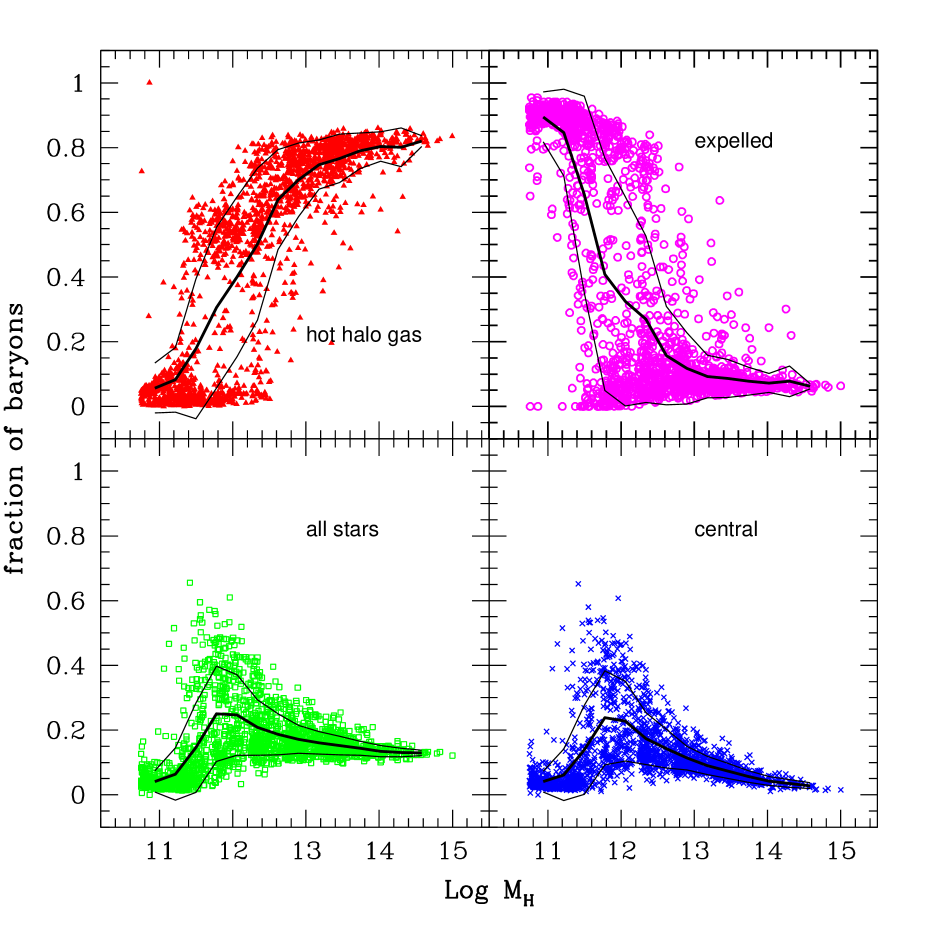
Figure 6: DM halos at $z=0$: fraction of baryons in hot halo gas (red triangles, upper left panel), expelled by winds (magenta circles, upper right panel), in stars in all galaxies (green open squares, lower left panel), in stars in the central galaxy (blue crosses, lower right panel). Averages and rms of the points are shown in all panels.

We find that the stellar mass of the typical central galaxy contained in the smallest DM halos at $z=0$ is $3\times 10^{8}$ M_⊙, so the stellar mass function is severely incomplete below this limit.

To limit the size of the output and the computing time, the mass function of DM halos is sampled by picking no more than 300 halos per mass bin of 0.5 dex (or all halos in the bin if they are less than 300). The statistical distributions of galaxies are then computed by weighting each galaxy by $w_{\rm tree}$, the inverse of the fraction of the host DM halos picked up in the mass bin. For each DM halo all galaxies and satellites are computed, so that for a given stellar mass the satellites of large DM halos are oversampled with respect to the central galaxies, which are numerically dominant at all masses. This feature shows up when galaxy properties are reported for samples of model galaxies, like in the Tully-Fisher relation: at fixed stellar mass, satellite galaxies with a low weight $w_{\rm tree}$ are more numerous in the plot than central galaxies with a high $w_{\rm tree}$. We then further sparse-sample the satellites as follows: we compute the average stellar mass of central galaxies as a function of the DM halo mass, then assign to each satellite a weight $w_{\rm gal}$ equal to the ratio between the $w_{\rm tree}$ of the average DM halo hosting a central galaxy with the same stellar mass and the $w_{\rm tree}$ of the host DM halo. We then select the satellite with a probability equal to $1/w_{\rm gal}$. In this way we obtain a roughly constant number of galaxies per logarithmic interval of stellar mass.

Figure 6 gives, for each selected DM halo evolved to $z=0$, the fraction of baryons that are found in hot halo gas, in stars of all galaxies (but not in the halo), in stars of the central galaxy, and the fraction of baryons ejected by winds and not fallen back. These clearly do not exhaust the list of baryonic components (halo stars and cold gas components are excluded here), so these fractions do not add up to one. However, this figure helps in showing a number of important features. There is a clear transition at a DM halo mass range of $10^{12}-10^{13}$ M_⊙: smaller halos lose most of their baryons by ejecting them to the IGM and their stellar content is dominated by the central galaxy, while larger halos retain most of their baryons as hot gas and have a small fraction of stars ($\sim 20$ per cent) in the central galaxy. In both cases the fraction of stars (both total and in the central galaxy) declines quickly with increasing or decreasing mass, while a maximum is reached at $10^{12}$ M_⊙. All these features reproduce nicely the trends suggested in the seminal papers of galaxy formation (see, for instance, White & Rees 1978 or Dekel & Silk 1986): small halos are evacuated by winds driven by SNe, while in large halos the large cooling time (aided by AGN feedback) prevents most gas from cooling. As a further element, it is worth noting the presence of many Milky Way-sized halos with almost no hot gas, in nice agreement with the lack of X-ray emitting around our Galaxy.

The trends of decreasing efficiency of star formation in smaller and larger halos than $10^{12}$ M_⊙ are needed to produce the observed low-luminosity slope and high-luminosity cutoff of the galaxy LFs. Figure 7 shows the predicted stellar mass function of galaxies, compared with the data by the 2dF$+$2MASS (Cole et al. 2001) and SDSS (Bell et al. 2003) surveys. The low-mass slope is nicely reproduced (though the result is sensitive to resolution, see appendix B) , even in the slight steepening below $10^{10}$ M_⊙. The high-mass cutoff is not strong enough, and the biggest ellipticals are too massive by at most a factor of two; however, this excess may be connected, as proposed by Monaco et al. (2006), to the construction of the diffuse stellar component of galaxy clusters, and would be fixed by a proper modeling of the scattering of stars during mergers (section 4.3); this work is in progress. We also report in the figure the resulting mass function without AGN feedback, to show that the quenching of the cooling flow by AGN jets decreases significantly the discrepancy with observations.

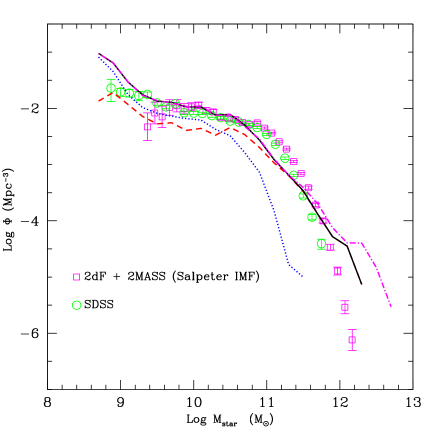
Figure 7: Stellar mass function of galaxies at $z=0$ (continuous black line), compared with the results of 2dF$+$2MASS (Cole et al. 2001) and SDSS (Bell et al. 2003). The dashed red and dotted blue lines give respectively bulge-dominated and disc-dominated galaxies, while the dot-dashed magenta line refers to a model without quenching of the cooling flows by AGN jets ($f_{\rm jet,0}=0$).

Figure 7 shows also the stellar mass function of bulge- and disc-dominated galaxies (these are very similar to the mass functions of bulges and discs). In line with what is observed, bulges dominate at large masses, while discs are more abundant at small masses. However, as noticed also by Croton et al. (2006), the mass function of bulges does not have a broad peak at $\sim 10^{10}-10^{11}$ M_⊙, as shown by the luminosity function of ellipticals; there is a definite excess of small bulges. This is likely connected to the excess in the predicted number density of $10^{10}$ M_⊙ galaxies at $z\sim 1$ reported by Fontana et al. (2006), a problem shared by many galaxy formation models. This point will be deepened in Fontanot et al. (2006b).

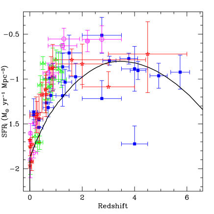
Figure 8: Star formation rate density as a function of redshift, compared with the data compiled and homogenized by Hopkins (2004). Points denote star formation estimates based on rest-frame UV (blue squares), $[{\rm O}II]$ (green triangles), H$\alpha$ and H$\beta$ (magenta circles), X-ray, FIR and sub-mm (red stars).

Figure 8 shows the prediction of the star formation rate density as a function of redshift. The data have been collected and homogenized by Hopkins (2004). The prediction is consistent with the data, with some possible underestimate at $z\sim 1$. In particular, a very broad peak of star formation is predicted to be present at $z\sim 3$, in agreement with the estimates based on sub-mm counts. The level of star formation is still high at $z\sim 6$, only a factor of 2 lower than the peak value; however, this prediction depends sensitively on the mass resolution. Most of this star formation takes place in discs, triggered by the strong cooling flows at high redshift, while mergers dominate the strongest starbursts; this will be deepened in Fontanot et al. (2006b).

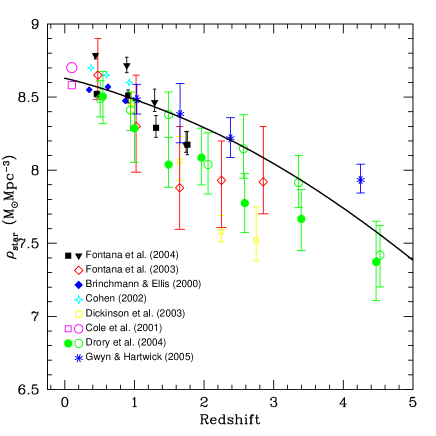
Figure 9: Stellar mass density as a function of redshift, compared with the data by Brinchmann & Ellis (2000), Cole et al. (2001), Cohen (2002), Dickinson et al. (2003), Fontana et al. (2003; 2004), Drory et al. (2004), Gwinn & Hartwick (2005). The data are not homogenized for the different sample completeness.

Figure 9 shows the cosmic stellar mass density as a function of redshift. Though this quantity is related to the cosmic star formation rate (it is simply its integral in time), it is compared with a completely different set of data (Brinchmann & Ellis 2000; Cole et al. 2001; Cohen 2002; Dickinson et al. 2003; Fontana et al. 2003, 2004; Drory et al. 2004; Gwinn & Hartwick 2005). The data in this figure are not homogenized for the different mass limits, so each point should be considered as a lower limit. The agreement with data is again good from $z\sim 4$ to 0. A more refined analysis of the build-up of the stellar mass is reported in Fontana et al. (2006) and Fontanot et al. (2006b).

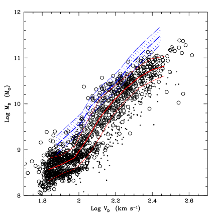
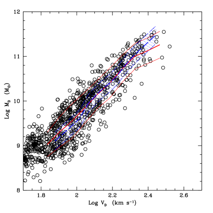
Figure 10: Baryonic Tully-Fisher relation for disc-dominated galaxies at $z=0$, compared with the relation obtained from the Universal Rotation Curve (Persic, Salucci & Stel 1996; Yegorova & Salucci 2006), shown as a shaded area. Dots and circles correspond respectively to discs with a gas fraction smaller and higher than 1 per cent. Continuous lines give the average (thick line) and average$\,\pm\,$rms (thin lines) of the circles. Left panel: standard model; right panel: model with concentration scaled to $c_{\rm nfw}=4$ for $10^{12}$ M_⊙ DM halos at $z=0$.

Figure 10 (left panel) shows the baryonic Tully-Fisher relation for the disc-dominated galaxies, where disc velocities $V_{\rm D}$ are computed at the optical radius (3.2$R_{\rm D}$) and $M_{\rm D}$ is the total disc mass. This relation is compared with that obtained from the universal rotation curve (Persic, Salucci & Stel 1996, updated by Yegorova & Salucci 2006); the intrinsic scatter around this relation is reported by the authors to be $\sim$0.2 dex. As a first point, there is a tail of rapidly spinning discs that are not seen in the data. These discs are formed at high redshift (when DM halos were denser and discs more compact), then become satellites so that no further infall on the disc takes place. Consequently, they are compact and gas-poor, and thus can hardly be classified as spirals. This is demonstrated in the figure, where all objects with a gas fraction lower than 1 per cent are denoted as small dots; most if not all outliers are then removed by applying this selection. As a second point, the gas-rich discs follow a Tully-Fisher relation parallel to the observed one but with a higher velocity by 0.1 dex, or 25 per cent, in $V_{\rm D}$. (Notably, galaxies follow the same Tully-Fisher relation independently of their surface brightness.) We have verified that no realistic combination of feedback parameters leads to a better zero-point of the relation. This disagreement is more likely related to the shape of the halo; for instance, Mo & Mao (2000) suggest that a concentration as low as $c_{\rm nfw}=4$ is required to fit the Tully-Fisher relation. To test this hypothesis we then scaled all concentrations by a constant factor so as to take a value of 4 for a $10^{12}$ M_⊙ halo at $z=0$. The resulting relation (figure 10, right panel) shows a much better agreement with the observed one (this change does not affect much the other galaxy properties, but ellipticals result larger and less dense as well). We then conclude that the disagreement in the zero-point of the baryonic Tully-Fisher relation is likely due to the inner profile of the DM halo more than to feedback. As a third and final point, the scatter around the Tully-Fisher relation is found to be $\sim$0.25 dex, possibly higher than what is suggested by data.

It must be stressed that this model was run without the computation of adiabatic contraction of the halo (section 6.1). We have verified that this further process, besides slowing down the computation significantly, makes the discs slightly more compact, without influencing drastically the other results; in fact, taking into account the presence of a bulge leads to a significant contraction in many discs, so that the adiabatic contraction of the halo does add much to this effect.

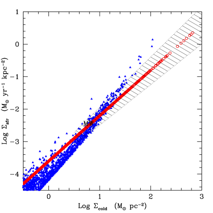
Figure 11: Schmidt-Kennicutt law for the disc (blue triangles) and bulge (red circles) components. The shaded area gives the observed relation reported by Kennicutt (1998).

Figure 11 shows the surface densities of cold gas versus star formation rate for discs and bulges, compared with the Schmidt-Kennicutt law (Kennicutt 1998). By construction, bulges stay exactly on the average relation, while discs follow the star-formation timescale of equation 58, which, as anticipated, gives a relation compatible with the observed one in virtue of the correlation between cold gas fraction and surface density. The agreement is very good both in terms of zero-point (apart from a marginal underestimate that could be easily fixed by a better tuning) and in terms of scatter.

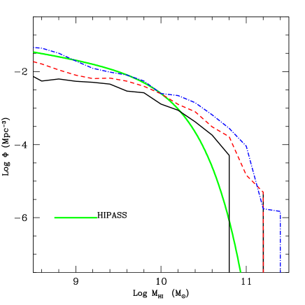
Figure 12: Mass function of HI gas (black continuous line), compared with the analytic fit of the results of the HIPASS sample (Zwaan et al. 2003; green thick line), assuming that the correction for helium and molecular gas amounts to a factor of 2. The statistical error of the observed mass function is very small. The dashed red and dot-dashed blue lines give the results of models with a threshold for star formation ($\Sigma_{\rm thr}=10$ M_⊙ pc^-2); in the blue dot-dashed model DM halo concentrations $c_{\rm nfw}$ are scaled so as to assume a value of 4 for a $10^{12}$ M_⊙ halo at $z=0$.

Figure 12 shows the prediction of the mass function of HI at $z=0$, compared with that obtained from the HIPASS sample (Zwaan et al. 2003). The statistical error of the observational mass function (well fit by a Schechter function) is so small for this sample that we do not even report it in the figure; conversely, the transformation from HI to total cold gas mass is rather uncertain. Following Fukugita & Peebles (2004), the HI and molecular gas densities at $z=0$ amount to $\Omega_{HI}=(3.5\pm 0.8)\times 10^{-4}$ (Zwaan et al. 2003) and $\Omega_{H_{2}}=(1.6\pm 0.4)\times 10^{-4}$ (Keres, Yun & Young 2003), so that, taking into account the abundance of helium (another 1.38 factor) the fraction of cold gas results a factor of two higher than that of HI; this is the conversion factor used in figure 12. With the standard choice of parameters morgana does not reproduce this mass function either at small or at large masses. In appendix B we show that the cutoff of this function is remarkably sensitive to mass resolution and decreases with decreasing particle mass, so that at this stage we decide not to give credit to the discrepancy at large masses. At smaller masses, we find that the amount of gas is sensitive both to the threshold for star formation $\Sigma_{\rm thr}$ introduced in section 7.2 and to the assumed star-formation law. Given the good reproduction of the Schmidt-Kennicutt law (even with a marginal underestimate of the star-formation rate, which would imply an increase of gas masses), the discrepancy in the amount of cold gas cannot be due to an error in the star-formation time-scale at a given $\Sigma_{\rm cold,D}$, but can be due to an error in the size of discs, which influences the value of $\Sigma_{\rm cold,D}$ and then of $t_{\star\rm,D}$. Such an error is also suggested by the discrepancy, reported above, in the zero-point of the baryonic Tully-Fisher. We then show two more models in figure 12, both with $\Sigma_{\rm thr}=5$ M_⊙ pc^-2, the second one with concentrations scaled to take a value $c_{\rm nfw}=4$ for a $10^{12}$ DM halo at $z=0$. Clearly, adding a threshold for star formation helps in increasing the amount of cold gas (under the assumption that the correction for the HI gas given above applies also beyond the threshold for star formation) but cannot solve the discrepancy, while the $c_{\rm nfw}=4$ case leads even to a satisfactory prediction of the low-end of the gas mass function. We conclude that the mass function of cold gas gives a very important fine constraint to the model, and that it gives further support to the idea that the NFW profile of DM halos leads to too compact discs. However, the uncertainty in the relation between HI and cold gas must be better taken into account before reaching strong conclusions.

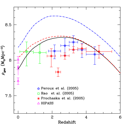
Figure 13: Evolution of the cold gas density, compared with the HIPASS point at $z=0$ (with and without the correction for helium and molecular gas) and to estimates of HI gas density from DLAs, obtained by Péroux et al. (2005), Rao et al. (2005) and Prochaska, et al. (2005). Model lines are as in figure 12.

Figure 13 shows the evolution of the cold gas density, compared with the HIPASS point (shown with and without the correction for molecular gas and helium) and the data from DLA systems (Péroux et al. 2005; Rao et al. 2005; Prochaska, Herbert-Fort & Wolfe 2005), to which no correction has been applied. The same three models as in figure 12 are shown. All the models show the same trend of a broad peak at $z\sim 2-4$ and a decrease by a factor of $\sim 5$ at $z<2$; the $c_{\rm nfw}=4$ model gives a remarkably high normalization. The data themselves are characterized by large errorbars and by a discrepancy between the Prochaska et al (2005) and Péroux et al. (2005) datapoints at $z\sim 2.5$. No strong conclusion can then be drawn from this figure, apart from a rough qualitative agreement.

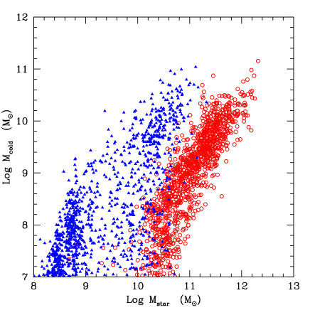
Figure 14: Gas content of disc-dominated (blue triangles) and bulge-dominated (red triangles) galaxies as a function of stellar mass.

Figure 14 shows, for the standard model, how cold gas is distributed in disc-dominated or bulge-dominated galaxies. Regarding the latters, while small ellipticals have a low gas content, the most massive objects have a significant gas load; at variance with what appears in the plot, they do not dominate the high end of gas mass function because they are hosted with the rare but well sampled massive DM halos. This excess of cold gas does not contribute much in terms of mass, but makes these galaxies too blue, thus highlighting that our quenching of the cooling flow by AGN feedback is not strong enough. This point will be addressed in more detail in a forthcoming paper.

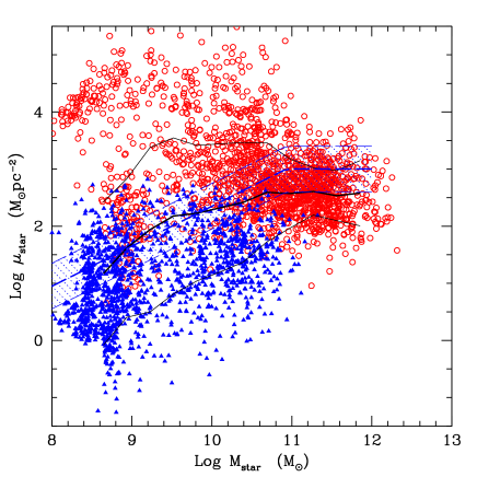
Figure 15: Stellar mass versus stellar surface density for disc-dominated (blue triangles) and bulge-dominated (red circles) galaxies in the model. The thick and thin continuous lines give the average and average$\,\pm\,$rms of the galaxies. The shaded area reports the observational result of Kauffmann et al. (2003).

Figure 15 shows the galaxies in the stellar mass–surface density plane. Spiral discs and bulges tend to occupy different regions of the plane; the scatter is however so strong that, as observed, no clear bimodality emerges from the distribution of these galaxies. The region occupied by SDSS galaxies in this plot (Kauffmann et al. 2003) is highlighted in the figure. A decrease of the surface brightness at masses $<10^{10}$ M_⊙ is obtained, in good agreement with the SDSS data; however, model galaxies are much more scattered.

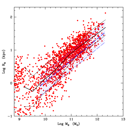
Figure 16: Half-mass radii of elliptical galaxies as a function of stellar mass. Points with errorbars give the average and rms in bins of the model galaxies. The lines give the the average and rms values of the data obtained from Marconi & Hunt (2003).

Figure 16 shows the bulge-dominated galaxies in the stellar mass–$R_{\rm B}$ plane, compared with the observed relation obtained from the data of Marconi & Hunt (2003), $R_{\rm B}=4.9(M_{\rm B}/10^{11}\ {\rm M}_{\odot})^{0.65}$ kpc (see also Monaco & Fontanot 2005), with a scatter of 0.3 dex. The data lie nicely within the observed range, with some flattening at small masses which is consistent with the findings of Graham et al. (2006). We do not show a prediction of the fundamental plane at this stage, because the virial theorem is implicit in our relation between mass, radius and velocity dispersion, and the computation of ${\cal M/L}$ ratios need a spectro-photometric code to be computed.

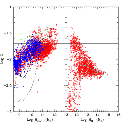
Figure 17: Left panel: metallicity of bulge-dominated (red points) and disc-dominated (blue triangles) galaxies, compared to the average and rms range of data of SDSS galaxies (Gallazzi et al. 2005, black dashed lines) and of the NOAO survey cluster ellipticals (Nelan et al. 2005, green dotted lines). Right panel: predicted metallicity of the hot halo component; in this panel, the continuous thick and thin cyan lines give the average and rms of the points.

Figure 17 shows the predicted metallicity of bulges, discs and hot halo gas. Elliptical galaxies show a mass-metallicity relation that steepens at masses smaller than $11^{10}$ M_⊙, spirals show a similar though weaker trend. These metallicities are compared with the results of Nelan et al. (2005), relative to the cluster elliptical galaxies of the NOAO fundamental plane survey, and Gallazzi et al. (2005), relative to SDSS galaxies. Both datasets suggest an increase of metallicity with stellar mass, which confirms our qualitative prediction, but they differ remarkably in the normalization. This reflects the intrinsic difficulties in estimating ages and metallicities in large samples of galaxies. Taking this into account, we notice that the region of masses lower than $\sim 3\times 10^{10}$ M_⊙ and metallicities lower than 0.005 is populated by SDSS galaxies (presumably by disc-dominated objects) but not by our model. Taking this result at face value, these data suggest that there may be a need of feedback in small-mass discs. In Figure 17 we also show the predicted metallicity of hot halo gas, which is enriched to a level of roughly $Z_{\odot}/3$ in clusters, which raises in galaxy groups and then is dominated by scatter at smaller DM halo masses (which are also almost devoid of hot gas). This is in qualitative agreement with the observed trend (Baumgartner et al. 2005) of an increase of metallicity from galaxy clusters to groups of 2-3 keV ($\sim 10^{14}$ M_⊙), possibly followed by a decrease at smaller masses.

13 Discussion and conclusions

We have presented and described in detail the code morgana for the formation and evolution of galaxies and AGNs. The most relevant features of morgana have been mentioned in the Introduction: it attempts, through its original modeling of cooling, star formation, feedback, galactic winds and super-winds, AGN activity and AGN feedback, to move from a phenomenological description of galaxy formation, based on simple scalings with the properties of the host DM halo, toward a fully physically motivated one. The numerical integration of the mass, energy and metal flows allows a wide set of physical processes to be straighforwardly implemented, and the multi-phase description of the inter-stellar and intra-cluster media, although used only in a limited way, is a step forward towards a more realistic description of the complex physics involved.

Despite many significant technical differences, the predictions of morgana at $z=0$ are in line with that of the other semi-analytical or N-body models: most of the figures shown in section 12, will be no real surprise for most experts of galaxy formation. Besides, a qualitative comparison of our results with the N-body ones of Tornatore et al. (2003) has shown in many cases the same trends, as for instance the formation of too massive ellipticals in clusters or the inability of stripping to produce a sufficient number of halo stars (see also Monaco et al. 2006). Similarly, the hidden dependence of the results on mass resolution and the lack of a proper convergence is shared by the two methods. This implies that the field is reaching an interesting level of maturity, so that an increase in the level of sophistication in these models is justified.

In the Introduction we stated that we do not regard this model as a “theory of everything” for galaxies, but simply as a powerful tool to understand the complex nature of galaxies and to bridge in a realistic way the physical processes in play with the observations that can constrain them. It is then important to focus on the discrepancies with observations found in this paper, and to the insights on the physical processes that they provide.

The exponential cutoff of the luminosity function is only roughly reproduced, which implies that the quenching of the cooling flow by the AGN is not well modeled; a stronger indication is given by the excess of cold gas in large ellipticals. This is no surprise given the poor level of understanding of this process. Our quenching is performed by allowing gas to cool, form stars and accrete onto the BH, at variance with the choice of switching cooling off whenever some fiducial criterion is satisfied, like e.g. in Hatton et al (2003), Bower et al. (2006) or Croton et al. (2006), a choice that leads to better fits to the luminosity functions and correct red colours for the most massive galaxies. Besides, if the build-up of massive galaxies by consecutive mergers is slowed down by the creation of the diffuse stellar component in galaxy clusters, as proposed by Monaco et al. (2006), then the high end of the stellar mass function (but not galaxy colours) may be determined by gravitational processes more than by AGN feedback. This suggests that the longly known cutoff of the stellar mass function may still give surprises in the future.

Another well-known discrepancy arises in reproducing the zero-point of the baryonic Tully-Fisher relation. Our results support strongly the idea that this problem is not due to an unsuitable modeling of feedback but to the shape of the inner density profile of DM halos; the cusped NFW halos produce discs that are too compact (with $V_{\rm D}$ values higher by 25 per cent), while by scaling the halo concentration so as to assume the low value $c_{\rm nfw}=4$ for a $10^{12}$ M_⊙ DM halo at $z=0$, as suggested by Mo & Mao (2000), it is possible to recover the zero-point of the Tully-Fisher relation. Besides, the formation of galaxy discs is based on the (reasonable but still not fully demonstrated) assumptions of conservation of angular momentum and formation of exponential discs, and our model neglects important problems related to the distribution of angular momentum within the DM halos. Given the complexity of this topic, it is remarkable that the observed Tully-Fisher relation is wrong by only 0.1 dex under the simplest assumptions.

The discrepancy in disc sizes is reflected also in the mass function of cold gas; model disc galaxies have correct stellar masses and stay on the correct Schmidt-Kennicutt law, but show a deficit of cold gas mass. This lack is partially fixed by inserting a threshold for star formation, but only the formation of less compact discs (hosted in flatter DM halos) can solve the discrepancy. Our analysis also shows the potentiality of using the mass function of cold gas in galaxies to test galaxy formation models, although the uncertainty in the relation between HI and total cold gas hampers strong conclusions.

Another point of disagreement with data is given by the excess of small bulges at $z=0$. This is related to the excess of $10^{10}$ M_⊙ galaxies at $z\ga 1$ (Fontana et al. 2006), and to the intrinsic difficulty of “downsizing” the AGN population (Fontanot et al. 2006a). The lack of low-metallicity discs may add to this evidence. These connected problems point to some missing feedback sources that acts in disc-dominated galaxies at high redshift (those that later merge to form bulges).

All these discrepancies point to the need of a deeper understanding of the complex process of galaxy formation, that will necessarily need a focus on the details of the various processes involved. In this regard, observations of larger and larger samples of galaxies will need to be complemented by detailed observations of objects where feedback is at work. To bridge together the two sets of evidences it will be necessary to use galaxy formation models that, on the one hand, are able to generate predictions for large samples of objects and, on the other hand, contain a sophisticated enough treatment of gas dynamics to make predictions on the detailed properties of galaxies. morgana is a contribution in this direction.

Appendix A Merging and destruction times for galaxies

The merging and destruction times are computed using the physically motivated analytic fits (accurate to $\sim 15$ per cent) of Taffoni et al. (2003) to the merging and destruction times found using N-body simulations and analytical models. We use here a version of the analytic fits that differs slightly from the one proposed in that paper in the values of the fitting parameters:

Let the merging halos have mass, circular velocities, virial radii and concentrations respectively $M_{\rm H}$, $V_{\rm H}$, $r_{\rm H}$, $c_{\rm H}$ (main halo) and $M_{\rm S}$, $V_{\rm S}$, $r_{\rm S}$, $c_{\rm S}$ (satellite). Let $f_{\rm sat}=M_{\rm S,0}/M_{\rm H}$ be the ratio between the initial mass of the satellite and the halo mass (we recall that the halo mass includes the satellite), and let $\epsilon$ and $x_{c}$ be the orbital parameters of the satellite (see section 4.1). In the case of a rigid satellite that suffers no mass loss, the dynamical friction time (the time required by an orbit to decay) is:

$$\tau_{\rm rigid}=0.46\frac{r_{\rm H}^{2}V_{\rm H}}{GM_{\rm S,0}}\left(1.7265+0.0416c_{\rm H}\right)\frac{x_{c}^{1.5}}{\ln\left(1+1/f_{\rm sat}\right)}$$ (84)

while for a live satellite, i.e. a satellite that suffers significant mass loss by tidal stripping, the dynamical friction time is:

$$\tau_{\rm live} = \frac{r_{\rm H}^{2}V_{\rm H}}{GM_{\rm S,0}}\times\left[{\cal B}f_{\rm sat}^{0.12}+{\cal C}f_{\rm sat}^{2}\right]$$

$$\times\left[0.25\left(c_{\rm H}/c_{\rm S}\right)^{6}-0.07(c_{\rm S}/c_{\rm H})+1.123\right]$$

$$\times\left[0.4+\left(\epsilon-0.2\right){\cal Q}\right]$$

where

$${\cal B} = -0.0504+0.3355x_{c}+0.3281x_{c}^{2}$$ (86)

$${\cal C} = 2.151-14.176x_{c}+27.383x_{c}^{2}$$ (87)

$${\cal Q} = 0.9+10^{8}\left(f_{\rm sat}-0.0077/(1-1.08x_{c})-0.0362\right)^{6}$$ (88)

$$\left(12.84+3.04x_{c}-23.4x_{c}^{2}\right)$$

The general expression for the dynamical friction time is obtained by interpolating between the two expressions: for $f_{\rm sat}>0.1$:

$$\tau_{\rm df}=\tau_{\rm rigid}\,;$$ (89)

for $0.08<f_{\rm sat}\leq 0.1$:

$$\tau_{\rm df}=\tau_{\rm rigid}\left(\frac{f_{\rm sat}-0.08}{0.02}\right)+\tau_{\rm live}\left(1-\frac{f_{\rm sat}-0.08}{0.02}\right)\,;$$ (90)

for $0.007<f_{\rm sat}\leq 0.08$:

$$\tau_{\rm df}=\tau_{\rm live}\,;$$ (91)

for $f_{\rm sat}\leq 0.007$:

$$\tau_{\rm df}=\max\left(2.1\tau_{\rm rigid}\epsilon^{0.475(1-\tanh(10.3f_{\rm sat}^{0.33}-7.5x_{c}))},\tau_{\rm live}\right)\,.$$ (92)

For the destruction times we follow closely Appendix B of Taffoni et al. (2003).

Appendix B Numerical stability

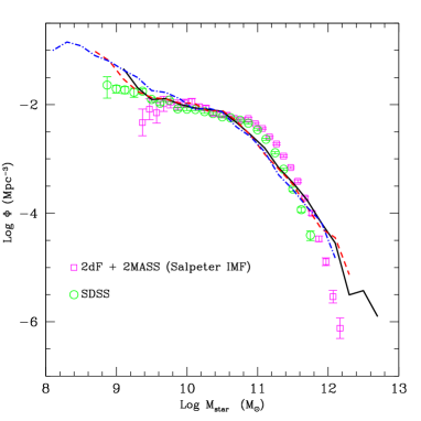
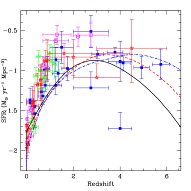
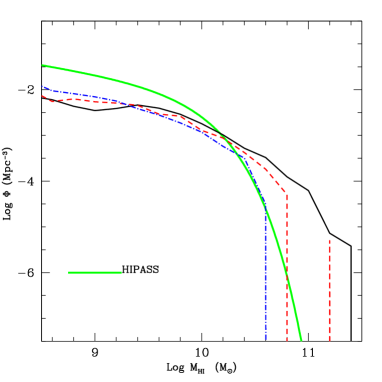
Figure 18: Stellar mass function (upper panel; see figure 7), star formation density (mid panel; see figure 8) and cold gas mass function (lower panel; see figure 12) for galaxies in the three runs with particle mass $3.0\times 10^{8}$ M_⊙ (blue dot-dashed lines), $1.0\times 10^{9}$ M_⊙ (red dashed line) and $2.4\times 10^{9}$ M_⊙ (black continuous line).

In this Appendix we show how some results are sensitive to the mass resolution of the merger trees. This is not to be considered as a complete convergence study, but only as a first test of the robustness of the results. Figure 18 gives the stellar mass function, star formation density and cold gas mass function for the three boxes introduced in section 12 and for the same set of parameters given in table 4.

The following conclusions can be drawn:

(i) the model roughly converges in predicting the stellar content of bright galaxies, but does not for small galaxies. In particular, at increasing resolution (decreasing particle mass) the stellar mass function gets steeper at the low-mass end and, as a consequence, lowers at the knee.

(ii) The star-formation density apparently converges at lower redshift, but gets increasingly large at $z\ga 2$. The main reason for the low-redshift convergence is that, to mimic the effect of reionization (following Benson et al. 2002; see section 2.6) cooling is quenched in halos with circular velocity larger than 50 km s^-1. The smallest sampled progenitor overtakes this limit at redshifts higher than 1, 2.8 and 7.5 for the three runs, in order of decreasing particle mass. This means that each box is missing star-forming halos at redshift higher than that limit, and explains why convergence in the star formation density is not visible in the figure.

(iii) From the stellar mass function and star-formation rate, it is clear that the excess of small-mass galaxies noticeable for the highest resolution run is connected to the excess of star formation at high redshift, so that the exceeding dwarf galaxies will be very old objects. This unwanted feature is clearly connected to the excess of galaxies with stellar mass $\la 10^{10}$ M_⊙ at $z\sim 1$ found by Fontana et al. (2006) by comparing models (including morgana) to the results of the GOODS-MUSIC survey, and to the excess of small bulges visible in figure 7. Clearly, a source of feedback, which would limit the formation of dwarf galaxies at $z>1$, is missing, and this lack is more and more evident when the particle mass decreases.

(iv) With the low-$V_{c}$ cutoff, convergence is reached in the star-formation rate at $z<1$, because only the run with the largest particle mass shows higher star formation density and a tail of galaxies more massive than $3\times 10^{12}$ M_⊙. This is related to the efficiency of the quenching of the late cooling flows by radio-loud AGNs. This demonstrates that our self-consistent quenching needs a particle mass not larger than $10^{9}$ M_⊙. In case of poor mass resolution it is possible to apply a procedure similar to Croton et al. (2006) and Bower et al. (2006) to force the quenching of the cooling flow. In this case, whenever a cooling flow is present it is assumed that a fraction of that flow would immediately accrete onto the BH (subject to the Eddington rate) and release energy to the hot halo phase. Whenever this “fiducial” energy is higher than that lost by cooling, quenching is switched off. This “forced cooling” procedure is clearly less physical than that described in section 9.2, and for a sufficiently small particle mass it gives a slightly stronger quenching of the cooling flows, but it can be considered as a rough numerical trick to achieve a good level of quenching when mass resolution is poor. This forced quenching procedure is used in Fontanot et al. (2006a).

(v) The high-mass cutoff of the cold gas mass function is the most sensitive prediction to mass resolution. We don’t find any hint of convergence for this quantity at $z=0$, despite the star content of the same galaxies is convergent. On the other hand, the low-mass tail of the same distribution is rather stable.

We can then conclude that the model does not really converge with the resolution, and that convergence at large masses is obtained by using Benson et al.’s motivated recipe. Some relevant ingredient, able to hamper star formation in small-mass (but relatively high circular velocity) galaxies at high redshift, is still missing.

References

- (1) Arnaboldi, M., Freeman, K.C., Okamura, S., et al., 2003, AJ, 125,514
- (2) Balland, C., Devriendt, J.E.G., Silk, J., 2003, MNRAS, 343, 107
- (3) Baugh, C.M., Lacey, C.G., Frenk, C.S., Granato, G.L., Silva, L., Bressan, A., Benson, A.J., Cole, S., 2005, MNRAS, 356, 1191
- (4) Baumgartner, W.H., Loewenstein, M., Horner, D.J., Mushotzky, R.F., 2005, ApJ, 620, 680
- (5) Bell, E.F., McIntosh, D.H., Katz, N., Weinberg, M.D., 2003, ApJS, 149, 289
- (6) Benson, A.J., Bower, R.G., Frenk, C.S., Lacey, C.G., Baugh, C.M., Cole, S., 2003, ApJ, 599, 38
- (7) Benson, A.J., Lacey, C.G., Baugh, C.M., Cole, S., Frenk, C.S., 2002, MNRAS, 333, 156
- (8) Bianchi, S., Cristiani, S., Kim, T.-S., 2001, A&A, 376, 1
- (9) Bond J.R., Cole S., Efstathiou G., Kaiser N., 1991, ApJ, 379, 440
- (10) Bower, R.G., Benson, A.J., Malbon, R., Helly, J.C., Frenk, C.S., Baugh, C.M., Cole, S., Lacey, C.G., 2006, submitted to MNRAS (astro-ph/0511338)
- (11) Brinchmann, J., Ellis, R.S., 2000, ApJL, 536, L77
- (12) Bullock, J.S., Dekel, A., Kolatt, T.S., Kravtsov, A.V., Klypin, A.A., Porciani, C., Primack, J.R., 2001, ApJ, 555, 240
- (13) Buchert T., Ehlers J., 1993, MNRAS, 264, 375
- (14) Cattaneo, A., Dekel, A., Devriendt, J., Guiderdoni, B., Blaizot, J., 2006, submitted to MNRAS (astro-ph/0601295)
- (15) Cavaliere, A., Vittorini, V., 2000, ApJ, 543, 599
- (16) Christodoulou, D.M., Shlosmann, I., Tohline J.E., 1995, ApJ, 443, 551
- (17) Cimatti, A.; Pozzetti, L.; Mignoli, M., et al., 2002, A&A, 391, L1
- (18) Cohen, J., 2002, ApJ, 567, 672
- (19) Cole, S., Lacey, C.G., Baugh, C.M., Frenk, C.S., 2000, MNRAS, 319, 168
- (20) Cole, S., Norberg, P., Baugh, C.M., et al., 2001, MNRAS, 326, 255
- (21) Cox, A.N., 2000, Allen’s astrophysical quantities, 4th ed. (New York: AIP Press). Pag. 572
- (22) Croton, D.J., Springel, V., White, S.D.M., et al., 2006, MNRAS, 365, 11
- (23) Dekel, A., Birnboim, Y., 2006, MNRAS, 368, 2
- (24) Dekel, A., Silk, J., 1986, ApJ, 303, 39
- (25) De Grandi, S., Molendi, S., 2002, ApJ, 567, 163
- (26) De Lucia, G., Springel, V., White, S.D.M., Croton, D., Kauffmann, G., 2006, MNRAS, 366, 499
- (27) Dickinson, M., Papovich, C., Ferguson, H.C., Budavári, T., 2003, ApJ, 587, 25
- (28) Dib, S., Bell, E., Burkert, A., 2006, ApJ, 638, 797
- (29) Di Matteo, T., Croft, R.A.C., Springel, V., Hernquist, L., 2003, ApJ, 593, 56
- (30) D’Onghia, E., Burkert, A., Murante, G., Khochfar, S., 2006, submitted to MNRAS (astro-ph/0602005)
- (31) Drory, N., Bender, R., Feulner, G., Hopp, U., Maraston, C., Snigula, J., Hill, G.J., 2004, ApJ, 608, 742
- (32) Efstathiou, G., Lake, G., Negroponte, J., 1982, MNRAS, 199, 1069
- (33) Eisenstein, D.J., Zehavi, I., Hogg, D.W., et al., 2005, ApJ, 633, 560
- (34) Eke, V.R., Navarro, J.F., Steinmetz, M., 2001, ApJ, 554, 114
- (35) Feldmeier, J.J., Ciardullo, R., Jacoby, G.H., Durrell, P.R., 2003, ApJS, 145, 65
- (36) Fontana, A., Donnarumma, I., Vanzella, E., et al., 2003, ApJL, 594, L9
- (37) Fontana, A., Pozzetti, L., Donnarumma, I., et al., 2004, A&A, 424, 23
- (38) Fontana, A., Salimbeni, S.,Grazian, A., et al., 2006, A&A, in press (astro-ph/0609068)
- (39) Fontanot, F., Monaco, P., Cristiani, S., Tozzi, P., 2006a, MNRAS, in press (astro-ph/0609823)
- (40) Fontanot, F., Monaco, P., Silva, L., et al., 2006b, in preparation
- (41) Genzel, R., Tacconi, L., Eisenhauer, F, et al., 2006, Nature, 442, 786
- (42) Fraternali, F., Cappi, M., Sancisi, R., Oosterloo, T., 2002, ApJ, 578, 109
- (43) Fukugita, M., Peebles, P.J.E., 2004, ApJ, 616, 643
- (44) Gallazzi, A., Charlot, S., Brinchmann, J., White, S.D.M., Tremonti, C.A., 2005, MNRAS, 362, 41
- (45) Gal-Yam, A., Maoz, D., Guhathakurta, P., Filippenko, A.V., 2003, AJ, 125, 1087
- (46) Governato, F., Mayer, L, Wadsley, J., Gardner J.P., Willman, B., Hayashi, E., Quinn, T., Stadel, J., Lake, G., 2004, ApJ, 607, 688
- (47) Governato, F., Willman, B., Mayer, L., Brooks, A., Stinson, Valenzuela, O., Wadsley, J., Quinn, T., 2006, submitted to MNRAS (astro-ph/0602351)
- (48) Graham, A.W., Merritt, D., Moore, B., Diemand, J., Terzic, B., 2006, AJ, in press (astro-ph/0608614)
- (49) Granato G.L., De Zotti G., Silva L., Bressan A., Danese L., 2004, ApJ, 600, 580
- (50) Granato G.L., Silva L., Monaco P., Panuzzo P., Salucci P., De Zotti G., Danese L., 2001, MNRAS, 324, 757
- (51) Gwyn, S.D.J., Hartwick, F.D.A., 2005, AJ, 130, 1337
- (52) Hatton S., Devriendt J.E.G., Ninin S., Bouchet F.R., Guiderdoni B., Vibert D., 2003, MNRAS, 343, 75
- (53) Hopkins, A.M., 2004, ApJ, 615, 209
- (54) Kang, X., Jing, Y.P., Mo, H.J., Börner, G., 2005, ApJ, 631 21
- (55) Kauffmann, G., Colberg, J.M., Diaferio, A., White, S.D.M., 1999, MNRAS, 303, 188
- (56) Kauffmann, G., Heckman, T.M., White, S.D.M., et al., 2003, MNRAS, 341, 54
- (57) Kazantzidis, S., Mayer, L., Colpi, M., Madau, P., Debattista, V.P., Wadsley, J., Stadel, J., Quinn, T., Moore, B., ApJ, 623, L67
- (58) Kennicutt, R.C.Jr., 1989, ApJ, 344, 685
- (59) Kennicutt, R.C.Jr., 1998, ApJ, 498, 541
- (60) Keres, D., Katz, N., Weinberg, D.H., Davé, R., 2005, MNRAS, 363, 2
- (61) Keres, D., Yun, M.S., Young, J.S., 2003, ApJ, 582, 659
- (62) Knop, R.A., Aldering, G., Amanullah, R., et al., 2003, ApJ, 598, 102
- (63) Kravtsov, A.V., 2003, ApJ, 590, L1
- (64) Lacey C., Cole S., 1993, MNRAS, 262, 627
- (65) Li, Yun, Mo, H.J., van den Bosch, F.C., 2005, submitted to MNRAS (astro-ph/0510372)
- (66) Lia, C., Portinari, L., Carraro, G., 2002, MNRAS, 330, 821
- (67) Mac Low, M.-M., 2003, in “Simulations of magnetohydrodynamic turbulence in astrophysics”, eds. E. Falgarone & T. Passot, Springer. pag. 182
- (68) Maller, A.H., Bullock, J.S., 2004, MNRAS, 355, 694
- (69) Marconi A., Hunt L.K., 2003, ApJ, 589, 21
- (70) Mathis, H., Lemson, G., Springel, V., Kauffmann, G., White, S.D.M., Eldar, A., Dekel, A., 2002, MNRAS, 333, 739
- (71) Menci, N., Cavaliere, A., Fontana, A., Giallongo, E., Poli, F., Vittorini, V., 2004, ApJ, 604, 12
- (72) Merloni, A., Heinz, S., Di Matteo, T., 2003, MNRAS, 345, 1057
- (73) McNamara, B.R., Nulsen, P.E.J., Wise, M.W., Rafferty, D.A., Carilli, C., Sarazin, C.L., Blanton, E.L., 2005, Nature, 433, 45
- (74) Mo, H.J., Mao, S., White, S.D.M., 1998, MNRAS, 295, 319
- (75) Mo, H.J., Mao, S., 2000, MNRAS, 318, 163
- (76) Monaco, P., 2004a, MNRAS, 352, 181 (M04)
- (77) Monaco, P., 2004b, MNRAS, 354, 151
- (78) Monaco, P., Fontanot, F., 2005, MNRAS, 359, 283
- (79) Monaco, P., Murante, G., Borgani, S., Fontanot, F., 2006, ApJ Letters, in press (astro-ph/0610045)
- (80) Monaco P., Salucci P., Danese L., 2000, MNRAS, 311, 279
- (81) Monaco, P., Theuns, T., Taffoni, G., Governato, F., Quinn, T., Stadel, J., 2002a, ApJ, 564, 8
- (82) Monaco P., Theuns T., Taffoni G., 2002b, MNRAS, 331, 587
- (83) Moore, B., Katz, N., Lake, G., Dressler, A., Oemler, A.Jr., 1996, Nature, 379, 613
- (84) Moutarde F.,Alimi J. M. ,Bouchet F. R.,Pellat R., Ramani A., 1991, ApJ, 382, 377
- (85) Murante, G., Arnaboldi, M., Gerhard, O., et al., 2004, ApJ, 607, L83
- (86) Nagashima, M., Lacey, C.G., Okamoto, T., Baugh, C.M., Frenk, C.S.; Cole, S., 2005, MNRAS, 363, L31s
- (87) Nagashima, M., Yahagi, H., Enoki, M., Yoshii, Y., Gouda, N., 2005, ApJ, 634, 26
- (88) Navarro J.F., Frenk C.S., White S.D.M., 1995, MNRAS, 275, 720
- (89) Nelan, J.E., Smith, R.J., Hudson, M.J., Wegner, G.A., Lucey, J.R., Moore, S.A.W., Quinney, S.J., Suntzeff, N.B., ApJ, 2005, 632 137
- (90) Ostriker, J.P., Bode, P., Babul, A., 2005, ApJ, 634 964
- (91) Pearce, F. R., Jenkins, A., Frenk, C.S., White, S.D.M., Thomas, P.A., Couchman, H.M.P., Peacock, J.A., Efstathiou, G., 2001, MNRAS, 326, 649
- (92) Percival W.J., Sutherland W.J., Peacock J.A., et al., 2002, MNRAS, 337, 1068
- (93) Perlmutter, S., Aldering, G., Goldhaber, G., et al. 1999, ApJ, 517, 565
- (94) P/’eroux, C., Dessauges-Zavadsky, M., D’Odorico, S., Kim, T.S., McMahon, R.G., 2005, MNRAS, 363, 479
- (95) Persic, M., Salucci, P., Stel, F., 1996, MNRAS, 281, 27
- (96) Press, W.H., Teukolsky, S.A., Vetterling, W.T., Flannery, B.P., 1992, Numerical recipes in FORTRAN, Cambridge: University Press
- (97) Prochaska, J., Herbert-Fort, S., Wolfe, A., 2005, ApJ, 635, 123
- (98) Rao, S.M., Prochaska, J.X., Howk, J.C., Wolfe, A.M., 2005, AJ, 129, 9
- (99) Recchi, S., Matteucci, F., D’Ercole, A., Tosi, M., 2002, A&A, 384, 799
- (100) Refregier, A., 2003, ARA&A, 41, 645
- (101) Rosati, P., Borgani, S., Norman, C., 2002, ARA&A, 40, 539
- (102) Schaye, J., 2004, ApJ, 609, 667
- (103) Schmidt M., 1959, ApJ, 129, 243
- (104) Silva, L., Granato, G.L., Bressan, A., Danese, L., 1998, ApJ, 509, 103
- (105) Somerville, R., Primack, J.R., 1999, MNRAS, 310, 1087
- (106) Spergel, D.N., Bean, R., Doré, O., et al., 2006, submitted to ApJ (astro-ph/0603449)
- (107) Spergel, D.N., Verde, L., Peiris, H. V., et al., 2003, ApJS, 148, 175
- (108) Springel, V., Hernquist, 2003, MNRAS 339, 289
- (109) Springel, V., White, S.D.M., Jenkins, A., et al., 2005, Nature, 435, 629
- (110) Steinmetz, M., Navarro, J.F., 2002, NewA, 7, 155
- (111) Sutherland R., Dopita M., 1993, ApJS, 88, 253
- (112) Suto, Y., Sasaki, S., Makino, N., 1998, ApJ, 509, 544
- (113) Taffoni G., Mayer L., Colpi M., Governato F., 2003, MNRAS, 341, 434
- (114) Taffoni G., Monaco P., Theuns T., 2002, MNRAS, 333, 623
- (115) Thomas D., Maraston, C., Bender, R., de Oliveira, C.M., 2005, ApJ, 621, 673
- (116) Toft, S., Rasmussen, J., Sommer-Larsen, J., Pedersen, K., 2002, MNRAS, 335, 799
- (117) Tormen, G., 1997, MNRAS, 290, 411
- (118) Tornatore, L., Borgani, S., Springel, V., Matteucci, F., Menci, N., Murante, G., 2003, MNRAS 342, 1025
- (119) Umemura M., 2001, ApJ, 560, L29
- (120) Viel, M., Haehnelt, M.G., Springel, V., 2004, MNRAS, 354, 684
- (121) Voit, G.M., Donahue, M., 2005, ApJ, 634, 955
- (122) Volonteri, M., Haardt, F., Madau, P., 2003, ApJ, 582, 559
- (123) Warren, M.S., Quinn, P.J., Salmon, J.K., Zurek, W.H., 1992, ApJ, 399, 405
- (124) Weinberg D.H., Hernquist L., Katz N., 2002, ApJ, 571, 15
- (125) White, S.D.M., Frenk, C.S., 1991, ApJ, 379, 52
- (126) White, S.D.M., Rees, M.J., 1978, MNRAS, 183, 341
- (127) Wu, K.K.S., Fabian, A.C., Nulsen, P.E.J., 2000, MNRAS, 318, 889
- (128) Yegorova, Y., Salucci, P., 2006, in preparation
- (129) Young, P.J., 1976, AJ, 81, 807
- (130) Zhao, D.H., Jing, Y.P., Mo, H.J., Börner, G., 2003, ApJ, 597, L9
- (131) Zibetti, S., White, S.D.M., Schneider, D.P., Brinkmann, J., 2005, MNRAS, 358, 949
- (132) Zwaan, M.A., Staveley-Smith, L., Koribalski, B.S., et al., 2003, AJ, 125, 2842