Can cellular convection in a rotating spherical shell maintain both global and local magnetic fields?

Abstract

A convection-driven MHD dynamo in a rotating spherical shell, with clearly defined structural elements in the flow and magnetic field, is simulated numerically. Such dynamos can be called deterministic, in contrast to those explicitly dependent on the assumed properties of turbulence. The cases most interesting from the standpoint of studying the nature of stellar magnetism demonstrate the following features. On a global scale, the convective flows can maintain a “general” magnetic field with a sign-alternating dipolar component. Local (in many cases, bipolar) magnetic structures are associated with convection cells. Disintegrating local structures change into background fields, which drift toward the poles. From time to time, reversals of the magnetic fields in the polar regions occur, as “new” background fields expel the “old” fields.

1 Introduction

The original motivation of this study was suggested by the problems of solar physics. Although the results obtained at this stage cannot be interpreted to represent the specifically solar dynamo process, we should give a brief exposition of the previous investigation that led us to the formulation of the problem considered here.

Observations of the solar magnetic fields reveal a bewildering variety of structures and activities. It is remarkable that solar processes vary in scale from sizes comparable to the solar radius to the limit of present resolution and in duration from tens of years to minutes (see, for instance, Schrijver and Zwaan [2000]).

Mean-field electrodynamics [Moffatt, 1978; Krause and Rädler, 1980] has clarified many issues concerning the generation of the global magnetic fields of cosmic bodies. However, such problems as the formation of local magnetic fields and their relationship to the global fields fall completely beyond the scope of mean-field theories. Meanwhile, the phenomenon of solar and stellar magnetism could be adequately understood only if the dynamics of the interplay between structures in the velocity field and magnetic field is comprehensively studied over a wide range of spatial scales. Dynamo models that are aimed at a unified description of the global and local processes and that deal with local, instantaneous quantities rather than averaged ones can naturally be referred to as “deterministic” models. They describe the structural elements present in the flow and in the magnetic field instead of considering the averaged parameters of the turbulent flow (in particular, the statistical predominance of one sign of the velocity-field helicity or another).

The idea that convection cells in the solar subphotospheric zone could be a connecting link between global and local magnetic fields traces back to the mid-1960s. Tverskoy [1966] represented the convection cell by a toroidal eddy and demonstrated, in the framework of a kinematic approach, that such a model convection cell can amplify the magnetic field and produce characteristic bipolar magnetic configurations. This approach was also used by Getling and Tverskoy [1971] to construct a kinematic model of the global dynamo in which toroidal eddies distributed over a spherical shell, acting jointly with the differential rotation of the shell, maintain a sign-alternating global magnetic field. If a poloidal magnetic field is present, the differential rotation produces a toroidal component of the global magnetic field. If the local magnetic configuration produced by an eddy interacting with the large-scale toroidal field is rotated through some angle about the axis of the eddy, this configuration contributes to the regeneration of the poloidal component of the global magnetic field. Thus, a cell locally interacting with the magnetic field serves in this model as a building block of the global dynamo, and the latter can in this case be called the “cellular” dynamo. The rotation of the local magnetic-field pattern can be expected if the system rotates as a whole and the flow is affected by the Coriolis force.

In recent years, after the advent of suitable computing facilities, some steps have been made to verify these ideas by means of numerical simulation. Getling [2001] and Getling and Ovchinnikov [2002] obtained numerical solutions to the three-dimensional nonlinear problem of magnetoconvection in a plane horizontal layer of incompressible fluid, heated from below, and found that hexagonal convection cells interacting with a weak initial (“seed”), horizontal magnetic field can produce various structures of the strongly amplified magnetic field, with a predominant bipolar component. Dobler and Getling [2004] extended this numerical analysis to compressible fluids and obtained similar results.

Modern computing resources make it possible to approach the development of numerical cellular-dynamo models that could provide a parallel description of both the global and local magnetic fields. However, even today, numerical schemes can hardly be used to simulate flows and magnetic fields over scale ranges covering two or more orders of magnitude. Only the largest convection cells — of sizes comparable to the depth of the convection zone (such as solar “giant” cells, for which little observational evidence exists) — can be simulated in the framework of global models. If we assume that the principal features of the process should be similar for convection on different scales, such global models would help us to verify our qualitative notion and provide guidelines for the elaboration of a more detailed description.

Here, we use numerical simulations to investigate the properties of cellular dynamos in rotating spherical shells, which could operate in stars under certain conditions. Although there are reasons to believe that the solar dynamo is also of the cellular type, we do not directly associate the presently obtained results with solar processes, since the computed patterns of magnetic-filed evolution bear only limited similarity to the pattern observed on the Sun. We merely note some remarkable features of the cellular dynamos, which may be of interest from the standpoint of stellar magnetohydrodynamics.

2 Formulation of the problem and numerical technique

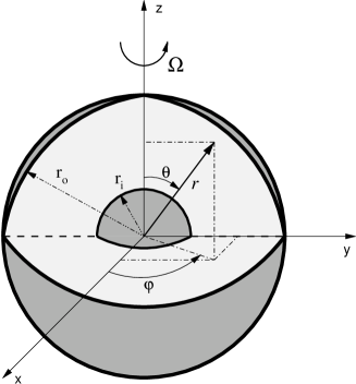
Figure 1: Geometrical configuration of the problem. The two spherical surfaces with radii $r_{\mathrm{i}}$ and $r_{\mathrm{o}}$ are dark-shaded. A part of the outer surface is removed to expose the interior of the shell (light-shaded) where the conducting fluid is confined.

In order to model the process of magnetic-field generation in a stellar convection zone, we consider a spherical shell of thickness $d=r_{\mathrm{o}}-r_{\mathrm{i}}$ (where $r_{\mathrm{o}}$ and $r_{\mathrm{i}}$ are the outer and inner radii of the shell), full of electrically conducting fluid and rotating with a constant angular velocity $\mathbf{\Omega}$ about a fixed axis $\hat{\mathbf{e}}_{z}$, as shown in Figure 1.

We follow the standard formulation used in earlier work by Tilgner and Busse [1997], Busse et al. [1998], Grote et al. [1999, 2000], and Simitev and Busse [2002, 2005], but we assume a more general form of the static temperature distribution,

$$T_{\mathrm{S}}=T_{0}-\frac{\beta}{2}d^{\,2}r^{2}+\frac{\beta_{1}}{d}\frac{1}{r},$$ (1)

$$\beta=\frac{q}{3\chi c_{p}},\quad\beta_{1}=\frac{\eta d\Delta T}{(1-\eta)^{2}},$$

where the radial coordinate $r$ is measured in units of $d$, $\chi$ is the thermal diffusivity, $c_{p}$ is the specific heat at constant pressure, $q$ is the mass density of uniformly distributed heat sources, $\eta\equiv r_{\mathrm{i}}/r_{\mathrm{o}}$ is the inner-to-outer radius ratio of the shell, and $T_{0}$ is a constant. The quantity $\Delta T$ is related to the difference between the constant temperatures of the inner and outer spherical boundaries, $T_{\mathrm{i}}$ and $T_{\mathrm{o}}$, as

$$\Delta T=T_{\mathrm{i}}-T_{\mathrm{o}}-\frac{1}{2}\beta d^{\,2}\frac{1+\eta}{1-\eta}$$ (2)

and reduces to $T_{\mathrm{i}}-T_{\mathrm{o}}$ in the case of $q=0$ (also dealt with in some simulations). The shell is self-gravitating, and the gravitational acceleration averaged over a spherical surface $r=\mathop{\mathrm{const}}\nolimits$ can be written as $\mathbf{g}=-\gamma d\cdot\mathbf{r}$, where $\mathbf{r}$ is the position vector with respect to the centre of the sphere; as specified above, its length $r$ is measured in units of $d$. In addition to $d$, the time $d^{2}/\nu$, the temperature $\nu^{2}/\gamma\alpha d^{4}$ (where $\alpha$ is the volumetric coefficient of thermal expansion), and the magnetic induction $\nu(\mu\rho)^{1/2}/d$ are used as scales for the dimensionless description of the problem; here, $\nu$ denotes the kinematic viscosity of the fluid, $\rho$ is its density, and $\mu$ is its magnetic permeability (we set $\mu=1$).

We use the Boussinesq approximation in that we assume $\rho$ to be constant except in the gravity term, where, in addition to the standard linear dependence $\rho(T)$ [according to which $\rho^{-1}(d\rho/dT)=-\alpha=\mathop{\mathrm{const}}\nolimits$], we introduce a small quadratic term in most cases. Once a cellular pattern has developed, the presence of this term and of the volumetric heat sources should not radically modify the properties of the dynamo; however, both these factors favour the development of polygonal convection cells [Busse, 2004] similar to the cells observed on the Sun, rather than meridionally stretched, banana-like convection rolls. Without these essential modifications, polygonal cells could only be obtained at much smaller rotational velocities; in this case, the process would develop very slowly, and the computations would be extremely time-consuming.

Thus, the equations of motion for the velocity vector $\mathbf{u}$, the heat equation for the deviation $\Theta$ from the static temperature distribution, and the equation of induction for the magnetic field $\mathbf{B}$ are

$$\nabla\cdot\mathbf{u}=0,$$ (3a)

$$(\partial_{t}+\mathbf{u}\cdot\nabla)\mathbf{u}=-\nabla\pi+\tau\mathbf{u}\times\hat{\mathbf{e}}_{z}+(\Theta+\epsilon\,\Theta^{2})\mathbf{r}$$

$$\hskip 71.13188pt+\nabla^{2}\mathbf{u}+(\nabla\times\mathbf{B})\times\mathbf{B},$$ (3b)

$$P\left(\partial_{t}+\mathbf{u}\cdot\nabla\right)\Theta=\nabla^{2}\Theta+\left(r_{\mathrm{i}}+R_{e}\frac{\eta}{(1-\eta)^{2}}\frac{1}{r^{3}}\right)\mathbf{r}\cdot\mathbf{u},$$ (3c)

$$\nabla\cdot\mathbf{B}=0,$$ (3d)

$$\partial_{t}\mathbf{B}=\nabla\times\left(\mathbf{u}\times\mathbf{B}\right)+P_{m}^{-1}\nabla^{2}\mathbf{B},$$ (3e)

where $\pi$ is an effective pressure.

Six nondimensional physical parameters of the problem appear in our formulation. The Rayleigh numbers measure the energy input into the system,

$$R_{\mathrm{i}}=\frac{\alpha\gamma\beta d^{\,6}}{\nu\chi},\qquad R_{\mathrm{e}}=\frac{\alpha\gamma\Delta Td^{\,4}}{\nu\chi},$$ (4)

and are associated with the internally distributed heat sources $q$ and the externally specified temperature difference $T_{\mathrm{i}}-T_{\mathrm{o}}$ [see equation (2)], respectively. The Coriolis number $\tau$, the Prandtl number $P$, and the magnetic Prandtl number $P_{\mathrm{m}}$ describe ratios between various time scales in the system,

$$\tau=\frac{2\Omega d^{\,2}}{\nu},\quad P=\frac{\nu}{\chi},\quad P_{\mathrm{m}}=\frac{\nu}{\nu_{\mathrm{m}}}$$ (5)

($\nu_{\mathrm{m}}$ is the magnetic viscosity, or magnetic diffusivity). Finally, $\epsilon$ is the small constant that specifies the magnitude of the quadratic term in the temperature dependence of density [see equation (3)].

Figure 2: Static profiles of the temperature and temperature gradient in the case of internal heating.

Since the velocity field $\mathbf{u}$ and the magnetic induction $\mathbf{B}$ are solenoidal vector fields, the general representation in terms of poloidal and toroidal components can be used,

$$\mathbf{u}=\nabla\times(\nabla v\times\mathbf{r})+\nabla w\times\mathbf{r},$$ (6a)

$$\mathbf{B}=\nabla\times(\nabla h\times\mathbf{r})+\nabla g\times\mathbf{r}.$$ (6b)

By multiplying the (curl)² and the curl of the Navier–Stokes equation (3) in the rotating system by $\mathbf{r}$, we obtain two equations for $v$ and $w$,

$$[(\nabla^{2}-\partial_{t}){\cal L}_{2}+\tau\partial_{\varphi}]\nabla^{2}v+\tau{\cal Q}w-{\cal L}_{2}(\Theta+\epsilon\,\Theta^{2})$$

$$\hskip 71.13188pt=-\mathbf{r}\cdot\nabla\times[\nabla\times(\mathbf{u}\cdot\nabla\mathbf{u}-\mathbf{B}\cdot\nabla\mathbf{B})]$$ (7a)

$$[(\nabla^{2}-\partial_{t}){\cal L}_{2}+\tau\partial_{\varphi}]w-\tau{\cal Q}v=\mathbf{r}\cdot\nabla\times(\mathbf{u}\cdot\nabla\mathbf{u}-\mathbf{B}\cdot\nabla\mathbf{B}),$$ (7b)

where $\varphi$ denotes the azimuthal angle (“longitude”) in the spherical system of coordinates $r,\theta,\varphi$, and the operators ${\cal L}_{2}$ and ${\cal Q}$ are defined by

$${\cal L}_{2}\equiv-r^{2}\nabla^{2}+\partial_{r}(r^{2}\partial_{r})\\$$

$${\cal Q}\equiv r\cos\theta\nabla^{2}-({\cal L}_{2}+r\partial_{r})(\cos\theta\partial_{r}-r^{-1}\sin\theta\partial_{\theta}).$$

The heat equation (3c) can be rewritten in the form

$$\nabla^{2}\Theta+\left[r_{\mathrm{i}}+R_{e}\eta r^{-3}(1-\eta)^{-2}\right]{\cal L}_{2}v=P(\partial_{t}+\mathbf{u}\cdot\nabla)\Theta.$$ (8)

Equations for $h$ and $g$ can be obtained multiplying the equation of magnetic induction (3e) and its curl by $\mathbf{r}$,

$$\nabla^{2}{\cal L}_{2}h=P_{m}[\partial_{t}{\cal L}_{2}h-\mathbf{r}\cdot\nabla\times(\mathbf{u}\times\mathbf{B})],$$ (9a)

$$\nabla^{2}{\cal L}_{2}g=P_{m}[\partial_{t}{\cal L}_{2}g-\mathbf{r}\cdot\nabla\times(\ \times(\mathbf{u}\times\mathbf{B}))].$$ (9b)

We assume stress-free boundaries with fixed temperatures,

$$v=\partial^{2}_{rr}v=\partial_{r}(w/r)=\Theta=0\mbox{ at }r=r_{\mathrm{i}}\mbox{ and }r=r_{\mathrm{o}}.$$ (10)

For the magnetic field, we use electrically insulating boundaries such that the poloidal function $h$ must be matched to the function $h^{(\mathrm{e})}$ that describes the potential fields outside the fluid shell

$$g=h-h^{(\mathrm{e})}=\partial_{r}(h-h^{(\mathrm{e})})=0\mbox{ at }r=r_{\mathrm{i}}\mbox{ and }r=r_{\mathrm{o}}.$$ (11)

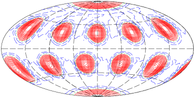
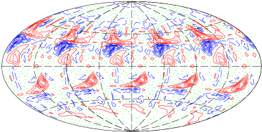
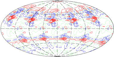
Figure 3: Contours of the radial velocity component on the sphere $r=r_{\mathrm{i}}+0.5$ at $t=98.73$ (top) and of the radial component of the magnetic field on the sphere $r=r_{\mathrm{o}}$ at $t=98.73$ (middle) and 101.73 (bottom) in the case of internal heating at $\eta=0.6$, $R_{\mathrm{i}}=3000$, $R_{\mathrm{e}}=-6000$, $\tau=10$, $P=1$, $P_{\mathrm{m}}=30$, and $m_{0}=5$. Solid (red) curves: positive values; dotted (green) curves: zero values; dashed curves (blue): negative values.

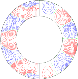
Figure 4: Contours of the axisymmetric azimuthal velocity (left-hand section) and streamlines of the meridional circulation, or contours of the stream function of the axisymmetric meridional flow (right-hand section) in the same case with internal heating ($P_{\mathrm{m}}=30$) at $t=98.73$. The curves have the same meaning as in Figure 3.

The numerical integration of equations (7)–(11) proceeds with a pseudospectral method developed by Tilgner and Busse [1997] and Tilgner [1998], which is based on an expansion of all dependent variables in spherical harmonics for the $\theta$ and $\varphi$ dependences; in particular, for the magnetic scalars,

$$g=\frac{1}{r}\sum_{l=0}^{\infty}\sum_{m=-l}^{l}G_{l}^{m}(r,t)P_{l}^{m}(\theta)\exp\{im\varphi\},$$ (12a)

$$h=\frac{1}{r}\sum_{l=0}^{\infty}\sum_{m=-l}^{l}H_{l}^{m}(r,t)P_{l}^{m}(\theta)\exp\{im\varphi\}$$ (12b)

(with truncating the series at an appropriate maximum $l$), where $P_{l}^{m}$ denotes the associated Legendre functions. For the $r$ dependences, truncated expansions in Chebyshev polynomials are used. The equations are time-stepped by treating all nonlinear terms explicitly with a second-order Adams–Bashforth scheme whereas all linear terms are included in an implicit Crank–Nicolson step.

For the computations to be reported here, a minimum of 33 collocation points in the radial direction and spherical harmonics up to the order 96 have been used. In addition to the geometric parameter $\eta$ and the above-mentioned physical parameters, we specified a computational parameter, viz., the fundamental (lowest nonzero) azimuthal number $m_{0}$. Thus, only the following azimuthal harmonics were really considered:

$$1,\ \mathrm{e}^{\pm\mathrm{i}m_{0}\varphi},\ \mathrm{e}^{\pm 2\mathrm{i}m_{0}\varphi},\ \mathrm{e}^{\pm 3\mathrm{i}m_{0}\varphi}\ldots\,.$$

In other words, we imposed an $m_{0}$-fold symmetry in the $\varphi$ direction. If $m_{0}\neq 1$, this reduces the computation time.

3 Results

3.1 Internal heating

For the cases of internal heating, we varied $P_{\mathrm{m}}$ and assumed $\eta=0.6$, $R_{\mathrm{i}}=3000$, $R_{\mathrm{e}}=-6000$, $\tau=10$, $P=1$, and $m_{0}=5$. As can be seen from checking computations with $m_{0}=1$ (not presented here), removing the artificially imposed fivefold azimuthal symmetry does not substantially modify the character of the convection pattern. The quadratic term was present in the temperature dependence of density, with a control parameter of $\epsilon=0.005$.

The distributions of the temperature $T_{\mathrm{S}}(r)$ and its gradient $\mathrm{d}T_{\mathrm{S}}/\mathrm{d}r$ for the corresponding static-equilibrium state are shown in Figure 2. Obviously, the outer part of the shell is convectively unstable and the inner part is stable.

3.1.1 The case of $\boldsymbol{P_{\mathrm{m}}=30}$.

At this $P_{\mathrm{m}}$ value, the computations covered a time interval of about 100 in units of the time of thermal diffusion across the shell. Over most part of this period, a very stable pattern of convection cells with a dodecahedral symmetry can be observed (Figure 3, top). These cells have a normal appearance typical of cellular convection, without substantial distortions due to the rotation of the shell. The entire pattern drifts in the retrograde direction, in agreement with theoretical predictions [Busse, 2004].

Figure 5: Variation in the amplitude of the dipolar harmonic of the poloidal magnetic field, $H_{1}^{0}(r,t)$, at $r=r_{\mathrm{i}}+0.5$ in the same case with internal heating ($P_{\mathrm{m}}=30$).

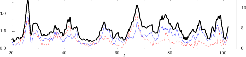
Figure 6: Density of magnetic energy and its particular fractions in the same case with internal heating ($P_{\mathrm{m}}=30$). Solid (heavy black) curve and right-hand vertical scale: total density of the magnetic energy; dashed (red) curve and left-hand vertical scale: energy density associated with the axisymmetric part of the magnetic-field component that has a dipole symmetry; dotted (blue) curve and left-hand scale: energy density associated with the nonaxisymmetric part of the same magnetic-field component.

The axisymmetric component of the azimuthal velocity (Figure 4) in a well-established flow pattern is nearly symmetric with respect to the equatorial plane. Specifically, a prograde rotation of the equatorial zone (in the frame of reference rotating together with the entire body) is present along with a retrograde rotation of the midlatitudes, and pairs of “secondary” prograde- and retrograde-rotation zones can also be noted in the polar regions. In a nonrotating frame of reference, the equatorial zone rotates more rapidly and the midlatitudinal zones more slowly than the shell as a whole does. Three pairs of meridional-circulation vortices fill the entire meridional section of the shell, from one pole to another.

The pattern of magnetic field is less regular than the pattern of flow (Figure 3, middle and bottom). Some remarkable features or the simulated dynamo process can be summarized as follows.

   

   

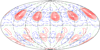
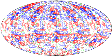
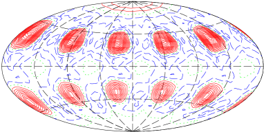
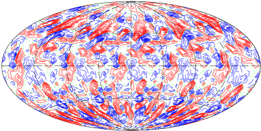
Figure 7: Contours of the radial component of the velocity on the sphere $r=r_{\mathrm{i}}+0.5$ (left) and of the magnetic field on the sphere $r=r_{\mathrm{o}}$ (right) at $t=200$ (top) and $t=327.2$ (bottom) in the case of internal heating at $P_{\textrm{m}}=200$, while the other parameters are as in the preceding case: $\eta=0.6$, $R_{\mathrm{i}}=3000$, $R_{\mathrm{e}}=-6000$, $\tau=10$, $P=1$, and $m_{0}=5$. The curves have the same meaning as in Figure 3.

Figure 8: Variation in amplitude of the dipolar harmonic of the poloidal magnetic field, $H_{1}^{0}(r,t)$, at $r=r_{\mathrm{i}}+0.5$ for the same case with internal heating as illustrated by Figure 7 ($P_{\mathrm{m}}=200$).

First, local magnetic structures associated with convection cells emerge repeatedly as compact magnetic regions (see Fig. 3). In their subsequent evolution, these regions change their configuration and finally dissipate into much weaker remnant fields.

Second, the dipolar component of the global magnetic field exhibits polarity reversals [see Figure 5 for a graph of the amplitude of the dipole component, $H_{1}^{0}(t)$]. The background fields — remnants of the decaying local magnetic structures — drift toward the poles and “expel” the “old” background fields present in the polar regions. As a result, the old magnetic polarity is replaced with the new one due to the poleward drift of the latter. The polarity reversals of the global magnetic field can also be seen from the variation in the amplitude of the dipolar harmonic of the poloidal field, $H_{1}^{0}(t)$ (Figure 5). The two maps of the magnetic field shown in Figure 3 correspond to two situations in which the global magnetic dipole has opposite orientations (the polarity reversal between these two times corresponds to the rightmost intersection of the curve in Figure 5 with the horizontal zero line).

Third, an interesting intermittent behaviour is exhibited by the magnetic energy of the system. Let us compare the full energy and two particular fractions of the energy associated with the magnetic-field component that has a dipolar-type symmetry (i.e., is antisymmetric with respect to the equatorial plane). Specifically, we are interested in the behaviour of the energy of the axisymmetric and the nonaxisymmetric part of this component. The axisymmetric part is represented by the spherical harmonics with $l$ odd and $m=0$ [see (12)], and the nonaxisymmetric part by other harmonics with $l+m$ odd. As can be seen from Figure 6 (in which the total energy and its particular fractions are divided by the volume of the shell), the main peaks in the graph of the total energy are alternately associated with increases in the energies of the axisymmetric and the nonaxisymmetric part of the component with a dipolar symmetry. In particular, the peak located near $t=42$ is fed by the symmetric field; near $t=55$, by the asymmetric field; near $t=68$, by both but with some predominance of the symmetric part; and near $t=78$, again by the asymmetric part.

3.1.2 The same case of $\boldsymbol{P_{\mathrm{m}}=30}$ but with special initial conditions.

In our attempts to find conditions for the realization of magnetic-field dynamics similar to the generally imagined pattern of a hypothetical dynamo process with differential rotation as its essential part (known since the qualitative model suggested by Babcock [1961] and Leighton [1964, 1969]), we made an additional computational run. We specified all parameters to be the same as in the above-described case. However, the initial conditions were chosen in such a way that, initially, the system would more likely find itself within the attraction basin of the expected dynamo regime in state space. To this end, we superposed the nonaxisymmetric components of the velocity field and magnetic field obtained in the above-described run onto a pattern of differential rotation with the equatorial belt accelerated compared to higher latitudes and with an appropriate distribution of the axisymmetric azimuthal magnetic field that has different signs on the two sides of the equator.

The computations have demonstrated that the system nevertheless approaches virtually the same regime that was observed without using such special initial conditions. Thus, a closer similarity between the numerical solution and the properties of the hypothetical dynamos of the Babcock–Leighton type does not seem to be achievable in the framework of this very simple model.

3.1.3 The case of $\boldsymbol{P_{\mathrm{m}}=200}$.

As the magnetic Prandtl number $P_{\mathrm{m}}$ is varied (under otherwise fixed conditions), the convection pattern varies little over a fairly wide $P_{\mathrm{m}}$ range. However, the greater this parameter, the higher the mean strength of the magnetic field (and, accordingly, the total magnetic energy). The kinetic energy of convection decreases with the increase of $P_{\mathrm{m}}$ and convection becomes more sensitive to time variations in the magnetic field. The increase of $P_{\mathrm{m}}$ is also manifest in the fact that local magnetic fields become more patchy and less ordered. Individual areas filled with the magnetic field of a given sign are smaller in size and more numerous, and bipolar structures are not so well pronounced (see Figure 7, which refers to $P_{\mathrm{m}}=200$). As in the case of $P_{\mathrm{m}}=30$, we can observe the penetration of background fields into the polar regions and sign reversals of the polar background fields.

Our computation for $P_{\mathrm{m}}=200$ cover a time interval almost five times as long as for $P_{\mathrm{m}}=30$ (Figure 8). The two velocity maps and two magnetic-field maps shown in Figure 7 nearly correspond to the times of one negative and one positive extremum of the amplitude $H_{1}^{0}(t)$ (see Figure 8). It is remarkable that the polar background fields have different polarities at these two times. At $t=200.0$, the background magnetic field is negative in the “northern” and positive in the “southern” polar region; an opposite situation takes place at $t=327.2$. The $H_{1}^{0}(t)$ curve demonstrates numerous sign reversals, although fine details of this dependence only reflect the irregular, fluctuational aspect of the process. It is nevertheless clear that, even if we smooth this curve, it will exhibit quite pronounced cyclic, although nonperiodic, polarity reversals of the dipolar component of the “general” magnetic field.

It should be noted that the distribution of the axisymmetric component of the azimuthal velocity (the pattern of differential rotation, not shown here) in this case is much more complex and variable than at $P_{\mathrm{m}}=30$. This effect also can be due to the stronger influence of the magnetic field on the fluid motion.

3.1.4 Internal heating without a $\boldsymbol{\Theta^{2}}$ term (nonmagnetic case).

To form an idea of the role played by the quadratic term in the $\rho(T)$ dependence, we computed a purely hydrodynamic (with $\mathbf{B}=0$) scenario under conditions that differed from the conditions of the above-described simulation by the absence of the $\Theta^{2}$ term ($\epsilon=0$) and by the Coriolis number ($\tau=1$); in addition, we assumed $m_{0}=1$ in this case.

The principal result of these computations is the finding that, in the absence of the quadratic term, convection unaffected by the magnetic field forms patterns of well-localized, three-dimensional cells, which typically appear as shown in Figure 9. A downwelling is observed in the centre of each cell, in contrast to the above-described cases, in which central upwellings typically developed. The issue of the direction of circulation in a convection cell is a fairly subtle matter (see, e.g., Getling [1999] for a survey of some situations related to convection in horizontal layers), so that agreement or disagreement between our model and any really observed pattern can in no way be an indication for the factors responsible for the observed direction of convective motions. Our primary interest in the cases where an upwelling is present in the central part of a cell is merely dictated by our intention of constructing a dynamo model reproducing the solar phenomena as closely as possible.

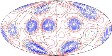
Figure 9: Contours of radial velocity on the surface $r=r_{\mathrm{i}}+0.5$ in the nonmagnetic case with internal heating, $\tau=1$; no quadratic term is present in the $\rho(T)$ dependence ($\epsilon=0$). The other parameters are $\eta=0.6$, $R_{\mathrm{i}}=3000$, $R_{\mathrm{e}}=-6000$, $P=1$ (as in the preceding cases), and $m_{0}=1$. The curves have the same meaning as in Figure 3.

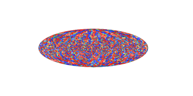
Figure 10: Map of the radial velocity component on the sphere $r=r_{\mathrm{i}}+0.5$ in the nonmagnetic case with heating through the inner boundary at $\eta=0.9$, $P=1$, $\tau=0.1$, $R_{\mathrm{e}}=5000$, and $m_{0}=2$. The contours merge into hatching: moderately light (red) for positive values, light (green) for zero values, and dark (blue) for negative values.

3.2 Heating “from outside” (through the inner surface)

In addition, we undertook a search for regimes in which convection preserves its “three-dimensional” structure in the absence of internal heat sources. In other words, some computations were done at $R_{\mathrm{i}}=0$. The quadratic term was also missing from the temperature dependence of density ($\epsilon=0$) in these runs.

Note that, in the limiting case of a nonrotating shell, convection cells are not stretched in any direction. Therefore, a cellular pattern of convective motion can obviously be maintained even without such favourable factors as a specific form of stratification and a quadratic term, but at smaller rotational velocities.

In shells without internal heat sources ($q=0$), convection regimes similar to those observed at $q\neq 0$ should be expected, under otherwise identical conditions, at smaller $\eta$. This is because a stratification similar to that shown in Figure 2 confines the development of convective motion to the outer part of the shell.

We illustrate here the case of $q=0$ only by a tentative computational run for convection without a magnetic field, at $\eta=0.9$, $P=1$, $\tau=0.1$, $R_{\mathrm{e}}=5000$, and $m_{0}=2$ (see Figure 10 for a velocity field typical of this case). Although the convection pattern is complex in this case, a tendency toward the formation of meridionally elongated cells can nevertheless be noted.

Computations with the magnetic field included (e.g., for $\eta=0.8$, $P=1$, $R_{\mathrm{e}}=5000$, $\tau=0.1$, $P_{\mathrm{m}}=5$) demonstrate the development of magnetic features with a very small spatial scale, close to the resolution limit of the computational scheme. This is a signature for an insufficient spatial resolution, so that the simulation results are not quite reliable.

The qualitative aspects of the results suggest that the Coriolis number proves again to be insufficiently small for the stability of “three-dimensional” convection cells, and the cells ultimately become substantially stretched, although not in a strictly meridional direction.

On the whole, the last two scenarios of flow and magnetic-field evolution indicate that regimes of “cellular” dynamo in a shell without internal heating and without a quadratic term in the $\rho(T)$ dependence should be sought in the range of smaller $\Omega$ (and $\tau$).

4 Conclusion

We have constructed relatively simple numerical models that describe a self-sustained process of generation of interacting global and local magnetic fields. As in most hypothetical astrophysical dynamos, the generation is driven by thermal convection in combination with differential rotation. We did not introduce any kinematic elements in our model, so that the entire velocity field appeared as the solution of the full system of MHD equations.

The most remarkable features revealed in the computed dynamo regimes can be summarized as follows. The process of magnetic-field generation is cyclic, although rather irregular. It includes the repeated generation of local, in many cases bipolar, magnetic structures. These structures dissipate giving rise to chaotic background fields. They may drift in the poleward direction, replacing the already existing, “old” background fields. In some cases, a correspondence can be noted between such polarity reversals in the polar regions and sign reversals of the axisymmetric bipolar component of the global magnetic field.

One of the computed scenarios demonstrates a remarkable intermittency in the behaviour of some fractions of magnetic energy: the axisymmetric and the nonaxisymmetric part of the magnetic-field component with a dipolar symmetry alternate in making larger contributions to the total-energy peaks.

Mean-field dynamo models, which have been most popular in astrophysics over a few past decades, attribute the generation of the global magnetic fields of stars to the $\alpha$ effect – the statistical predominance of one sign of the velocity-field helicity over another. It is quite plausible that the $\alpha$ effect, in one form or another, is a fairly general property of various velocity fields capable of maintaining undamped regular magnetic fields. However, this property must not necessarily be associated with turbulent motion. In particular, the model velocity field in the toroidal eddies used by Getling and Tverskoy [1971] to construct a global dynamo included an azimuthal (with respect to the axis of the eddy) velocity component, so that the trajectories of the fluid particles were spirals deformed in a certain way. A similar property may also be inherent in the convective flow that develops in our model, although checking this possibility requires a special investigation.

At this stage, the “deterministic” cellular dynamo described here is oversimplified to be regarded as a model of the solar or any other specific stellar dynamo. However, it demonstrates that the dynamics of the well-structured local magnetic fields and of the global magnetic field may be ingredients of one complex process.

The work of A.V.G. was supported by the Deutscher Akademischer Austauschdienst, European Graduate College “Non-Equilibrium Phenomena and Phase Transitions in Complex Systems,” and Russian Foundation for Basic Research (project code 04-02-16580).

References

Babcock, H. W. (1961), The topology of the sun’s magnetic field and the 22-year cycle, Astrophys. J., 133, 572.

Busse, F. H. (2002), Convective flows in rapidly rotating spheres and their dynamo action, Phys. Fluids, 14, 1301.

Busse, F. H. (2004), On thermal convection in slowly rotating systems, Chaos, 14, 803.

Busse, F. H., E. Grote, and A. Tilgner (1998), On convection driven dynamos in rotating spherical shells, Stud. Geophys. Geod., 42, 211.

Dobler, W., and A. V. Getling (2004), Compressible magnetoconvection as the local producer of solar-type magnetic structures, in Multi-Wavelength Investigations of Solar Activity, Proc. IAU Symp. No. 223, St. Petersburg, Russia, 2004, eds A. V. Stepanov, E. E. Benevolenskaya, A. G. Kosovichev. Cambridge Univ. Press, p. 239.

Getling, A. V. (1998), Rayleigh–Bénard Convection: Structures and Dynamics, World Scientific, Singapore [Russian version: URSS, Moscow, 1999].

Getling, A. V. (2001), Convective mechanism for the formation of photospheric magnetic fields, Astron. Zh., 78, 661 (Engl. transl: Astron. Rep., 45, 569, 2001).

Getling, A. V., and I. L. Ovchinnikov (2002), Solar convection as the producer of magnetic bipoles, in The 10th European Solar Physics Meeting “Solar Variability: From Core to Outer Frontiers,” Prague, Czech Republic, 2002 (ESA SP-506), vol. 2, p. 819.

Getling, A. V., and B. A. Tverskoy (1971), A model of the oscillatory hydromagnetic dynamo: I, II, Geomagn. Aeron., 11, 211, 389.

Grote, E., F. H. Busse, and A. Tilgner (1999), Convection-driven quadrupolar dynamos in rotating spherical shells, Phys. Rev. E, 60 , R5025.

Grote, E., F. H. Busse, and A. Tilgner (2000), Regular and chaotic spherical dynamos, Phys. Earth Planet. Inter., 117, 259.

Krause, F., and K.-H. Rädler (1980), Mean-Field Electrodynamics and Dynamo Theory, Akademie-Verlag, Berlin.

Leighton, R. B. (1964), Transport of magnetic fields on the sun, Astrophys. J., 140, 1547.

Leighton, R. B. (1969), A magneto-kinematic model of the solar cycle, Astrophys. J., 156, 1.

Moffatt, H. K. (1978), Magnetic Field Generation in Electrically Conducting Fluids, Cambridge Univ. Press, Cambridge.

Schrijver, C. J., and C. Zwaan (2000), Solar and Stellar Magnetic Activity, Cambridge Univ. Press, Cambridge.

Simitev, R., and F. H. Busse (2002), Parameter dependences in convection driven spherical dynamos, in High Performance Computing in Science and Engineering’02, eds E. Krause, W. Jäger, Springer, Heidelberg, p. 15.

Simitev, R., and F. H. Busse (2005), Prandtl number dependence of convection driven dynamos in rotating spherical fluid shells, J. Fluid Mech., 532, 365, .

Tilgner, A. (1999), Spectral methods for the simulation of incompressible flows in spherical shells, Int. J. Num. Meth. in Fluids, 30, 713, .

Tilgner, A., and F. H. Busse (1997), Finite–amplitude convection in rotating spherical fluid shells, J. Fluid Mech., 332, 359.

Tverskoy, B. A. (1966), Anent the theory of hydrodynamic self-excitation of regular magnetic fields, Geomagn. Aeron., 6, 11.

(Received 00.00.00; revised 00.00.00;

accepted 00.00.00)