Triple correlations in local helioseismology

Abstract

A central step in time-distance local helioseismology techniques is to obtain travel times of packets of wave signals between points or sets of points on the visible surface. Standard ways of determining group or phase travel times involve cross-correlating the signal between locations at the solar photosphere and determining the shift of the envelope of this cross correlation function, or a zero crossing, using a standard wavelet or a reference wave packet. Here a novel method is described which makes use of triple correlations, i.e. cross-correlating signal between three locations. By using an average triple correlation as reference, differential travel times can be extracted in a straightforward manner.

1 Introduction

Since the first realisation of the usefulness of time-distance helioseismology ([Duvall et al. 1993]) the technique has seen considerable application and has developed also in terms of the tools used to interpret the relationship between the time delays measured for wave packets travelling a specified horizontal distance and the perturbations in temperature and velocity fields below the visible surface. A recent review describing the current state of the subject is [Gizon & Birch 2005].

Time-distance helioseismic processing starts with the raw visible surface velocity data in the form of Dopplergrams and ends with performing the inverse problem to obtain tomographic images of sub-surface structures. An essential intermediate step is to carry out cross-correlation of velocity time series between locations where the relevant spectral line is formed, separated by one or more specified horizontal distances. Normally the cross-correlation is carried out between patches of pixels. e.g. centre-annulus or arc-to-arc cross-correlation, in order to improve the signal-to-noise ratio. Also, the signal is often pre-filtered, to let through only signals travelling at horizontal phase speeds confined within a small band.

The cross-correlation function typically takes the form of a wavelet centered at a certain delay time away from $0$, which is superposed on noise. Therefore one can fit e.g. a Morlet wavelet to this in order to extract the time of the maximum of the envelope, which is a proxy for the group travel time, or the time of a selected zero-crossing which is a proxy forn the phase travel time. These travel times are then the input for the inverse problem. Recently, an improvement of this technique has been proposed ([Gizon & Birch 2004]) where instead of a Morlet wavelet, a reference wavelet is used, for instance obtained from quiet Sun data, or computed from a reference solar model. The details of the fitting and time-delay extraction can be found in [Gizon & Birch 2004]. This technique is more robust in the sense that it continues to function at lower signal-to-noise ratios. Nevertheless it is still somewhat cumbersome and there is scope for alternative estimators for travel times. In this paper one possible alternative is discussed, which is based on triple correlations. In some sense the technique is carried over from for instance speckle masking interferometry where it has been applied succesfully for compensating for atmospheric seeing to achieve aperture-limited high spatial resolution imaging in a variety of settings (cf. [Lohmann, Weigelt & Wirnitzer 1983], [Bartelt, Lohmann & Wirnitzer 1984]).

2 Technique

The triple correlation of three time series $f_{1}$ $f_{2}$ and $f_{3}$ is defined as :

$$c(\tau_{1},\tau_{2})\equiv\int{\mathrm{d}}t\ f_{1}(t)f_{2}(t+\tau_{1})f_{3}(t+\tau_{2})\ .$$ (1)

This is most conveniently calculated in the Fourier domain where the Fourier transform $C$ of the correlation function $c$ is related to the Fourier transforms $F_{1}$, $F_{2}$ and $F_{3}$ of the three time series by taking their product as follows :

$$C(\omega_{1},\omega_{2})=F_{1}(\omega_{1})F_{2}(\omega_{2})F_{3}^{*}(\omega_{1}+\omega_{2})\ .$$ (2)

Although it is possible to calculate these triple products directly from the Fourier transform of single pixel time series, in the first instance the pre-processing is retained from the standard two-point cross correlations, using averaging masks to improve the signal-to-noise ratio and a phase speed filter to isolate a wave packet. This is done in order to compare the results of the two methods, and also in order to assess the sensitivity of the results to noise propagation, by adjusting the parameters of the masks and filters.

Figure 1: The weights in the averaging masks for the triple correlation shown as a linear color scale with red the smallest and white the largest relative weight. Note that the masks are all slightly displaced outward from the origin to bring out the structure more clearly.

A GONG (Global Oscillations Network Group) datacube, tracked at the solar rotation rate, and re-sampled onto a common spatial grid is used for testing purposes. This cube is Fourier transformed in the two spatial directions and in the time direction. The mask averaging is done conveniently in the Fourier domain, because of efficiency. If one needs to mask and average data using a mask with a fixed shape which is shifted around to sample the entire domain available, this can be expressed as a convolution. In the (spatial) Fourier domain the convolution becomes a simple multiplication of the spatial Fourier transform of the data and the Fourier transform of the mask. In this way all necessary averages are obtained at once. Also, the volume of data that is needed for subsequent steps is reduced drastically since it is now significantly oversampled in the spatial directions so that a lot of redundant data can be dropped from the subsequent steps in the analysis.

Similarly the application of the phase speed filter to the data is done by Fourier transforming the phase speed filter and multiplying through with the Fourier transformed data-cube. The phase speed filter $H$ used is Gaussian in shape :

$$H({\bf k},\omega)=\frac{2}{\Delta_{v}}\sqrt{\frac{\ln 2}{\pi}}\exp\left[-\frac{4\ln 2}{\Delta_{v}^{2}}\left(\frac{\omega}{|k|}-v_{\rm cen}\right)^{2}\right]\ .$$ (3)

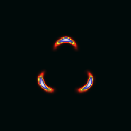
With this definition $\Delta_{v}$ corresponds to the full-width at half maximum (FWHM). The masks chosen for the three point correlation function are arcs. The centres of the three arcs are placed on an equilateral triangle at a distance corresponding to $29\ {\mathrm{Mm}}$. For the purposes of these feasibility tests only a single distance is used. For full tomographic inversions, a range of distances would be used, and the properties of the phase speed filter and mask would be adjusted accordingly. The weighting is not uniform over the arcs : the profile of the arc in the radial direction as well as in the azimuth angle is Gaussian, with a FWHM of $10\ {\mathrm{Mm}}$ and $90^{o}$ respectively. The masks are illustrated in Fig. 1 which shows as a color scale the averaging weight for the three arcs. Each arc is normalised to have a unit sum over the pixel weights. The parameters of the phase speed filter are set to :

$$v_{\rm cen} =44\ {\mathrm{km/s}}$$

$$\Delta_{v} =17.6\ {\mathrm{km/s}}\ .$$ (4)

Figure 2: In the Fourier domain a triple correlation fills a hexagonal area, bounded by the Nyquist frequency in $\omega_{1}$ $\omega_{2}$ and $\omega_{1}+\omega_{2}$, shown in the figure. Since the time series are real there is redundancy and only two quadrants need be manipulated. The arrows indicate which points are complex conjugate pairs.

Before discussing the results of the triple correlations it is useful to consider what one would expect. The time series are sampled at a finite rate, which implies that there is no information in the Fourier domain for frequencies that are in absolute value above the Nyquist frequency. In the domain of the two Fourier frequencies $\omega_{1},\omega_{2}$ (see Fig. 2) one can therefore restrict the analysis to a square region centered on the origin. Two triangles are further ‘cut away’ because these fall outside the Nyquist range for $\omega_{1}+\omega_{2}$. This hexagonal area contains the complex valued Fourier transform of the triple correlation function. Since the original time series, and therefore also their triple correlation, is real valued, points in this diagram that are mirror images with respect to the origin (see the arrows in Fig. 2) are complex conjugates.

$$C(-\omega_{1},-\omega_{2})\equiv C^{*}(\omega_{1},\omega_{2})$$ (5)

There is therefore no need to retain all 4 quadrants : two suffice and here the choice is made to retain quadrants 1 and 4. In speckle interferometry there are further symmetries in the quantities that are being correlated, with the consequence that the domain necessary to fully specify the information can be cut down further. That is not the case here ; the time series are not invariant under time reversal for instance, and therefore no further reduction is possible.

In the time domain, two-point correlation functions tend to have a wavelet shape superposed on noise. In the Fourier domain, two-point correlation functions are normally also structured with multiple peaks, and three point correlation functions therefore are as well. Most commonly in time-distance helioseismology, the shape of the wavelet is not used. The only parameter that is extracted is a time delay, either from a zero crossing or from the location of the maximum of an envelope. It is consistent with this to assume that to lowest order the shape of the triple correlation i.e. its complex modulus, does not change over a field of triple correlations. To this order, the only quantity of interest is the relative displacement of this wavelet to larger or smaller delays, which in the Fourier domain corresponds to a shift in the complex phase. In other words the triple correlation wavelet $w(\tau_{1},\tau_{2})$ in the time domain is presumed to be related to an (ensemble) average $\langle w\rangle(\tau_{1},\tau_{2})$ as :

$$w(\tau_{1},\tau_{2})=\int{\rm d}\tau^{\prime}_{1}\int{\rm d}\tau^{\prime}_{2} \langle w\rangle(\tau^{\prime}_{1},\tau^{\prime}_{2})\times$$ (6)

$$\,\delta(\tau^{\prime}_{1}-\tau_{1})\delta(\tau^{\prime}_{2}-\tau_{2})\ ,$$

in which the $\delta$ are Dirac delta functions. This describes a convolution and therefore can be expressed as a simple multiplication in the Fourier domain. This suggests an approach such as Wiener filtering, in which the Fourier transform of the triple correlation $W$ is divided by the Fourier transform of the ensemble averaged triple correlation $\langle W\rangle$. Then what one retains is the Fourier transforms of the two $\delta$-functions i.e. a function of the form $e^{i\phi}$ in which the complex phase $\phi$ is :

$$\phi=\omega_{1}\Delta_{1}+\omega_{2}\Delta_{2}\ .$$ (7)

The $\Delta_{1}$ and $\Delta_{2}$ are differences in travel time between and individual triple correlation and the average, as represented by the average triple correlation $\langle w\rangle$.

Figure 3: The modulus of the complex valued Fourier transform of the triple correlation in quadrants 1 and 4, when averaged over the entire $8\times 8$ field of triple correlations. The color scale is logarithmic covering 20 powers of 10 ; black and red representing smallest and blue and white largest values.

Figure 4: The complex phase of the Fourier transform of the triple correlation in quadrants 1 and 4, when averaged over the entire $8\times 8$ field of triple correlations. The color scale is linear : yellow is zero phase, red and black is negative phase, blue and white is positive phase.

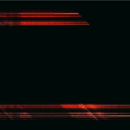
In Figs. 3 and 4 the complex modulus and phase are shown of the average triple correlation in the Fourier domain $\langle W\rangle$ obtained by averaging the Fourier amplitudes and phases over all of the $8\times 8$ triple correlations over the field covered by the data-cube. The phase is set to $0$ where the modulus is below a certain threshold. By construction the distances between the three points being correlated is the same and therefore one would expect the maximum correlation to occur for $\tau_{1}=\tau_{2}$ in the average correlation $\langle w\rangle$. In the Fourier domain this corresponds to structures aligned along $\omega_{1}+\omega_{2}=\mathrm{const.}$. For the same reason the individual cross correlations and the ratios $W/\langle W\rangle$ should show the same structure. This is particularly clear in Fig. 4. In Fig. 3 the modulus is high only in very localised regions so that such a structure is lost.

In calculating the ratio of triple correlations there is evidently a problem in large regions of the domain where the average $\langle W\rangle=0$. This is not an uncommon problem in inversions, and one expression of the need for regularisation in inverse problems. In this case the most straightforward regularisation is similar to what is done in singular value decomposition. Rather than using $W/\langle W\rangle$ one uses :

$$\Phi(\omega_{1},\omega_{2})=\frac{W(\omega_{1},\omega_{2})}{\langle W(\omega_{1},\omega_{2})\rangle+\epsilon}$$ (8)

where $\epsilon$ is a suitably small number which needs to be adjusted to the problem at hand. Here $\epsilon=10^{-13}$, which is small compared to the maximum value in the average triple correlation $\langle W\rangle_{\mathrm{max}}\sim 10^{16}$.

Figure 5: The modulus of the complex valued Fourier transform of the triple correlation ratio $\Phi$ in quadrants 1 and 4, at a location near the centre of the field. The color scale is logarithmic covering 5 powers of 10 with color coding as in Fig. 3.

Figure 6: The complex phase of the Fourier transform of the triple correlation ratio $\Phi$ in quadrants 1 and 4, at a location near the centre of the field. The color scale is linear : yellow is zero phase, red and black is negative phase, blue and white is positive phase.

Figure 7: The modulus of the complex valued Fourier transform of the triple correlation ratio $\Phi$ in quadrants 1 and 4, at the same location as Fig. 5 but without any filtering. The color scale is logarithmic covering 5 powers of 10 with color coding as in Fig. 3.

Figure 8: The modulus of the complex valued Fourier transform of the triple correlation ratio $\Phi$ in quadrants 1 and 4, at the same location as Fig. 5 but with a more localised mask. The color scale is logarithmic covering 5 powers of 10 with color coding as in Fig. 3.

If the shape of the wavelet were indeed constant over the field, and only displaced to larger or smaller relative time delays, the maps of the complex modulus of $\Phi$ would be featureless : equal to $1$ everywhere. The complex phase of $\Phi$ would show tructures aligned along $\omega_{1}+\omega_{2}=\mathrm{const.}$ as mentioned above. However, the group and phase travel time of waves both change over the field, but not necessarily by the same value, due to the fact that the dispersion relation is complex. Only if the sub-photospheric region of the Sun were to satisfy :

$$\frac{|\bf k|}{\omega}\frac{\partial\omega}{\partial|\bf k|}=\mathrm{const.}$$ (9)

would $\Phi$ show this behaviour. Since this is not the case, the modulus of $\Phi$ also shows structure, as does its phase.

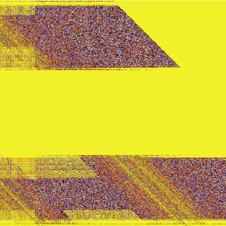
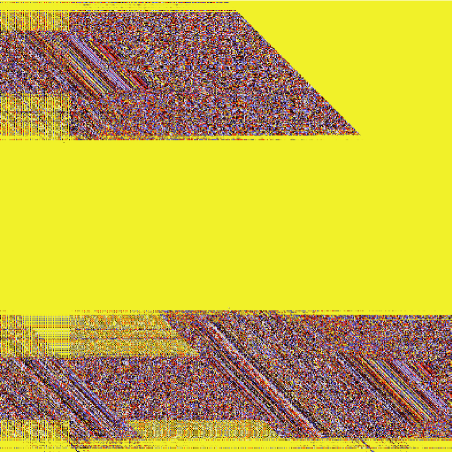
In Figs. 5 and 6 the triple correlation ratio in the Fourier domain $\Phi$ is shown for a single location near the centre of the field. Fig. 5 shows the logarithm of the modulus and Fig. 6 shows the phase. There are two clear ridges present as expected, both in the modulus and in the phase diagrams, from which a time-delay can be extracted. It is clear that along rdiges of $\omega_{1}+\omega_{2}=\mathrm{const.}$ there is little variation other than what is created because of the regularisation process. One can therefore integrate along the ridges and reduce the time-delay extraction to determining a single mean value $\tau_{1}=\tau_{2}=\tau_{\mathrm{m}}$ from the remaining 1-D Fourier transform.

3 Discussion & Conclusions

The triple correlation technique to extract relative time delays is demonstrated to function on a data-set obtained from GONG. The tests discussed in this paper are done on real data for an active region, with standard filtering and averaging applied and therefore it is evident that noise does not pose a significant problem in extracting time delays. However, further work is necessary to establish the relationship between the relative time delays recovered in this way, and the perturbations in sub-photospheric layers. As has been pointed out in [Gizon & Birch 2002] and in [Jensen & Pijpers 2003] it is possible to express this relationship in terms of a linear inverse problem with known kernels, as long as perturbations from a known equilibrium are small. However, the precise form that these kernels take does depend on the processing in terms of averaging and filtering. Although the differences with existing kernels are unlikely to be substantial, appropriate kernels for the triple correlation processing are still to be derived.

A point to note is that the time delays extracted are measured relative to the mean solar sub-photosphere over the time period covered by the data. This mean is not necessarily identical to a standard solar model. In order to be able to interpret the time delays with the appropriate kernels calculated from a standard model one should also extract the differential time delay of the average with respect to the standard solar model. This can be done by calculating the triple correlation $W_{\mathrm{mod}}$ as it would be for the model and extracting the delay from the (regularised) ratio $\langle W\rangle/(W_{\mathrm{mod}}+\epsilon)$. The reason to proceed in this way is that the average triple correlation $\langle W\rangle$ is a horizontal average for the region, for which a comparison with a (horizontally invariant) standard solar model is more straightforward to interpret. The horizontal perturbations measured by individual triple correlations are more likely to be linear when compared with a horizontal average, than they are when compared with a standard solar model.

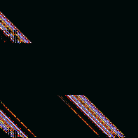
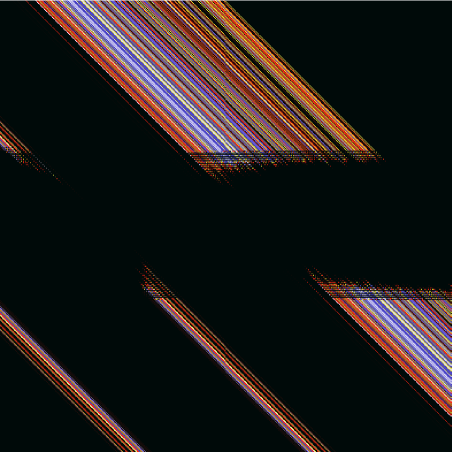
In order to illustrate the sensitivity to the filtering of the triple correlations, the same data-cube was processed but without using any filtering at all. The equivalent of Fig. 5 is shown in Fig. 7. It is clear that qualitatively similar structure is present in both images so that even for unfiltered data it would be possible to extract a relative time delay. However in the unfiltered processing the relative delays would be quite different from those recovered from filtered data. This is due to the fact that without the filtering there is a mixture of wave modes with very different depths of penetration into the sub-surface layers. The relative delays with respect to the mean appear to be much larger here, which suggests that these data are dominated by modes that remain in shallow layers, such as f modes. The influence of noise, either measurement noise or intrinsic solar noise, appears to be minimal.

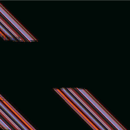
A separate test is to retain the filtering, but to reduce the extent of the averaging mask. In Fig. 8 both the radial extent and the azimuthal extent (FWHM) of the arcs is reduced by a factor of $\sqrt{2}$. This figure shows essentially the same structure as Fig. 5 although perhaps more of the expected periodic structure is present in the form of a third ridge, which implies that the time delay is somewhat better constrained for the smaller mask. Further optimisation of the combination of filtering and spatial averaging is in progress.

The computational burden of processing this data cube of 512 slices of 128x128 pixels is $12\ \mathrm{min}$ on an 8 processor machine. This is very similar to the standard two point correlation processing, with a more direct and robust access to the time delays. The preliminary tests with filtering and averaging indicate that perhaps less averaging is necessary compared to standard two-point correlation functions, which would be beneficial for subsequent tomography.