The Keck $+$ Magellan Survey for Lyman Limit Absorption I: The Frequency Distribution of Super Lyman Limit Systems

Abstract

We present the results of a survey for super Lyman limit systems (SLLS; defined to be absorbers with $19.0\leq$$\log N_{HI}$ $\leq 20.3$ cm^-2) from a large sample of high resolution spectra acquired using the Keck and Magellan telescopes. Specifically, we present 47 new SLLS from 113 QSO sightlines. We focus on the neutral hydrogen frequency distribution $f_{\rm{HI}}(N,X)$ of the SLLS and its moments, and compare these results with the Lyman–$\alpha$ forest and the damped Lyman alpha systems (DLA; absorbers with $\log N_{HI}$$\geq 20.3$ cm^-2). We find that that $f_{\rm{HI}}(N,X)$ of the SLLS can be reasonably described with a power-law of index $\alpha=-1.43^{+0.15}_{-0.16}$ or $\alpha=-1.19^{+0.20}_{-0.21}$ depending on whether we set the lower $N_{\rm HI}$ bound for the analysis at $10^{19.0}$cm^-2 or $10^{19.3}$cm^-2, respectively. The results indicate a flattening in the slope of $f_{\rm{HI}}(N,X)$ between the SLLS and DLA. We find little evidence for redshift evolution in the shape of $f_{\rm{HI}}(N,X)$ for the SLLS over the redshift range of the sample $1.68<z<4.47$ and only tentative evidence for evolution in the zeroth moment of $f_{\rm{HI}}(N,X)$, the line density $\ell_{\rm{SLLS}}(X)$. We introduce the observable distribution function ${\mathcal{O}}(N,X)$ and its moment, which elucidates comparisons of H I absorbers from the Lyman–$\alpha$ forest through to the DLA. We find that a simple three parameter function can fit ${\mathcal{O}}(N,X)$ over the range $17.0\leq$$\log N_{HI}$$\leq 22.0$. We use these results to predict that $f_{\rm{HI}}(N,X)$ must show two additional inflections below the SLLS regime to match the observed $f_{\rm{HI}}(N,X)$ distribution of the Lyman–$\alpha$ forest. Finally, we demonstrate that SLLS contribute a minor fraction $(\approx 15\%$) of the universe’s hydrogen atoms and, therefore, an even smaller fraction of the mass in predominantly neutral gas.

Accepted to ApJ; Revised October 30 2006

1 Introduction

For nearly three decades, the study of absorption line systems towards distant quasars has addressed a wide range of astrophysical and cosmological issues. These systems are typically classified according to their neutral hydrogen content: the Ly$\alpha$ forest absorbers with $\log N_{HI}$$\leq 17.2$ cm^-2, the Lyman limit systems (LLS) with $17.2\leq$$\log N_{HI}$$\leq 20.3$ cm^-2, and the damped Lyman alpha systems (DLA) with $\log N_{HI}$$\geq 20.3$ cm^-2. Both the Ly$\alpha$ forest and DLA absorbers have received considerable attention. The Ly$\alpha$ forest can be used to constrain cosmological parameters through a number of methods, such as through studies of the flux power spectrum (Croft et al., 2002; McDonald et al., 2005), the mean flux decrement (Tytler et al., 2004), or the distribution in column density and velocity width of the absorbers (e.g. Kirkman & Tytler, 1997; Kim et al., 2002). The DLA trace the bulk of the neutral gas at high redshift and are believed to be the progenitors of modern day galaxies (Wolfe, Gawiser & Prochaska, 2005). Large statistical samples of both the Ly$\alpha$ forest and the DLA are readily observed because their $N_{\rm HI}$ is easily determined. For the Ly$\alpha$ forest, the $N_{\rm HI}$ is determined directly from Voigt profile fits to the Ly$\alpha$ line which is dominated by the Maxwellian profile, or from higher order Lyman transitions when Ly$\alpha$ is saturated. For the DLA, the Lorentzian component of the Voigt profile gives pronounced damping wings, allowing for accurate $N_{\rm HI}$ determinations from spectra even at low signal to noise or resolution.

Recently, Prochaska, Herbert-Fort, & Wolfe (2005, hereafter PHW2005) analyzed the thousands of spectra from the Sloan Digital Sky Survey (SDSS) Data Release 3, and determined the $N_{\rm HI}$ frequency distribution for over 500 DLA systems. In contrast, there exists comparatively little study of the LLS. Surveys for LLS absorption (Tytler, 1982; Sargent, Steidel & Boksenberg, 1989; Lanzetta, 1991; Storrie-Lombardi et al., 1994; Stengler-Larrea et al., 1995) have concentrated primarily on the frequency of absorption with redshift (frequently expressed as $dn/dz$ or $dN/dz$, but we adopt the notation $\ell(z)$ for the line density which was introduced by PHW2005), but not on the $N_{\rm HI}$ value of the LLS. These surveys generally included the full range of H I column density of $\log N_{HI}\geq 17.2$ cm^-2 in $\ell(z)$. As such, the surveys also contained the $\ell(z)$ of DLA systems.

Our ignorance of LLS largely stems from the fact that accurate determinations of $N_{\rm HI}$ for the LLS are difficult compared to the Ly$\alpha$ forest and the DLA. In part, this is because the LLS systems represent the flat portion of the curve of growth for the Ly$\alpha$ transition and a precise $N_{\rm HI}$ measurement requires high resolution observations (e.g. Steidel, 1990). For most LLS, the $N_{\rm HI}$ is determined by using the information from the Lyman limit, either by looking at the differential flux level above and below the limit, or by the spacing of the lines as they approach the Lyman limit, or both (e.g. Burles & Tytler, 1998). The differential flux method requires a detailed understanding of the continuum flux level which is difficult to obtain in high redshift QSOs, and the line spacing technique requires a precise model for the hydrogen velocity structure, which can generally only be inferred from the metal lines associated with the LLS (e.g. Kirkman et al., 2003). These challenges are particularly acute for low-resolution observations where the Lyman series is poorly resolved.

Because the frequency of intersecting a LLS is observed to be of order one per sightline at redshifts $z>2.5$ (Storrie-Lombardi et al., 1994), a relatively large QSO sample is required in comparison with Ly$\alpha$ forest studies. At redshifts $z>3.25$, the SDSS provides just such a sample (Adelman-McCarthy et al., 2006), offering many thousands of sightlines suitable for analysis of LLS. Unfortunately, the SDSS spectra are of too poor a resolution to provide useful constraints on the $N_{\rm HI}$ for the LLS which are optically thick, i.e. $\log N_{HI}$$\geq 17.5$ cm^-2. To address this nearly three decade gap in $N_{\rm HI}$, we have pursued a high-resolution survey for LLS using telescopes in both the northern and southern hemisphere. The goal of this survey is to obtain high–resolution, high–SNR spectra of at least 100 LLS, with full coverage over the LLS $N_{\rm HI}$ range. In this paper, we discuss a sub–sample of this survey, namely the LLS with $\log N_{HI}$$\geq 19.0$ cm^-2. The lower bound on $N_{\rm HI}$ is chosen such that systems with this column density can be easily identified and analyzed in moderate to high resolution data (FWHM $<50$ km s^-1; Dessauges-Zavadsky et al., 2003). The $N_{\rm HI}$ values for these LLS are determined from the damping wings present in the Ly$\alpha$ line, in a fashion analogous with DLA analysis in lower resolution spectra. Previous work on this subset of the LLS population referred to the absorption systems as ‘sub-DLAs’. Because the majority of these absorbers are likely to be predominantly ionized (e.g. Viegas, 1995; Prochaska, 1999), we adopt the nomenclature of Prochaska & Herbert-Fort (2004) for those LLS exhibiting $\log N_{HI}$$\geq 19.0$ cm^-2: the ‘super Lyman limit’ or SLLS absorbers.

The fundamental measure of a class of QAL systems is the H I column density frequency distribution $f_{\rm{HI}}(N,X)$, defined to be the number of absorbers in the column density interval $(N,N+dN)$ identified along the cosmological distance interval $(X,X+dX)$ with $dX\equiv\frac{H_{0}}{H(z)}(1+z)^{2}dz$. This quantity, the absorption distance, is generally evaluated across a redshift interval $\Delta z$. The $f_{\rm{HI}}(N,X)$ distribution for QAL systems is analogous to the luminosity function of galaxy surveys. Moments of $f_{\rm{HI}}(N,X)$ give important quantities such as the line density of absorption systems, and the mass density of H I atoms. The $f_{\rm{HI}}(N,X)$ distribution is the starting point for assessing the baryonic mass density of these absorbers as well as their cosmological metal budget. The frequency distribution of LLS is of particular interest because the $N_{\rm HI}=10^{17}-10^{20}\,{\rm cm^{-2}}$ interval is expected to include the $N_{\rm HI}$ value where QAL systems transition from primarily neutral gas to predominantly ionized gas (e.g. Zheng & Miralda-Escudé, 2002, ; PHW05). Furthermore, Prochaska et al. (2006) have argued that the LLS can constitute a considerable fraction of the metals in the young universe (see also Péroux et al., 2006). At $z\simeq 2$, a census for metals which includes the DLA, stars in high–$z$ galaxies, and the IGM falls short by up to 70% of the total predicted metal mass density (e.g. Bouché, Lehnert & Péroux, 2006).

The primary goal for this study of the SLLS is to extend the statistics we use to describe the Lyman–$\alpha$ forest and the DLA into regions of H I column density which are currently poorly constrained (see also Péroux et al., 2003, 2005). By doing so, we hope to place the SLLS within the larger framework of high redshift QSO absorption line systems, and to explore their cosmological significance. Future papers will examine the ionization state, chemical abundances, and other physical properties of these absorbers. Throughout the paper, we adopt values of the cosmological parameters consistent with the latest Wilkinson Microwave Anisotropy Probe (WMAP) results (Bennett et al., 2003): $\Omega_{\Lambda}$$=0.7$, $\Omega_{m}$$=0.3$, and $H_{0}=70$ km s^-1 Mpc^-1.

Table 1: MIKE QUASAR SAMPLE

Name	RA (J2000)	DEC (J2000)	$z_{em}$	$z_{start}$	$z_{end}$	$z_{mask}^{a}$
Q0001-2340	00:03:45.00	$-$23:23:46.5	2.262	1.780	2.228	2.187
Q0101-304	01:03:55.30	$-$30:09:46.0	3.137	1.941	3.095
SDSS0106+0048	01:06:19.24	$+$00:48:23.3	4.433	2.997	4.378
SDSS0124+0044	01:24:14.80	$+$00:45:36.2	3.807	2.292	3.758
SDSS0147-1014	01:45:16.59	$-$09:45:17.3	2.138	1.797	2.106
SDSS0209-0005	02:09:50.70	$-$00:05:06.4	2.856	1.879	2.816	2.523
SDSS0244-0816	02:44:47.78	$-$08:16:06.1	4.047	2.829	3.996
HE0340-2612	03:42:27.80	$-$26:02:43.0	3.082	2.016	3.040
SDSS0912+0547	09:12:10.35	$+$05:47:42.0	3.248	2.146	3.205
SDSS0942+0422	09:42:02.04	$+$04:22:44.6	3.273	1.896	3.229
HE0940-1050	09:42:53.40	$-$11:04:25.0	3.067	1.944	3.025
SDSS0949+0355	09:49:32.27	$+$03:35:31.7	4.097	2.636	4.045
SDSS1025+0452	10:25:09.64	$+$04:52:46.7	3.236	2.108	3.193
SDSS1032+0541	10:32:49.88	$+$05:41:18.3	2.843	1.826	2.804
CTS0291	10:33:59.90	$-$25:14:26.7	2.552	1.747	2.515
SDSS1034+0358	10:34:56.31	$+$03:58:59.3	3.367	2.208	3.322
Q1100-264	11:03:25.60	$-$26:45:06.1	2.140	1.747	2.108
HS1104+0452	11:07:08.40	$+$04:36:18.0	2.660	1.747	2.622
SDSS1110+0244	11:10:08.61	$+$02:44:58.1	4.149	3.367	4.097
SDSS1155+0530	11:55:38.60	$+$05:30:50.5	3.464	2.282	3.418
SDSS1201+0116	12:01:44.36	$+$01:16:11.5	3.215	2.002	3.172
LB1213+0922	12:15:39.60	$+$09:06:08.0	2.713	1.796	2.675
Q1224-0812	12:26:37.50	$-$08:29:29.0	2.142	1.747	2.110
SDSS1249-0159	12:49:57.24	$-$01:59:28.8	3.662	2.406	3.614
SDSS1307+0422	13:07:56.73	$+$04:22:15.5	3.026	1.821	2.985
LBQS1334-0033	13:36:46.80	$-$00:48:54.2	2.809	1.829	2.770
SDSS1336-0048	13:36:47.14	$-$00:48:57.2	2.806	1.796	2.767
SDSS1339+0548	13:39:41.95	$+$05:48:22.1	2.969	1.969	2.928
HE1347-2457	13:50:38.90	$-$25:12:17.0	2.599	1.749	2.562
Q1358+1154	14:00:39.10	$+$11:20:22.3	2.578	1.747	2.541
SDSS1402+0146	14:02:48.07	$+$01:46:34.1	4.187	2.618	4.134
SDSS1429-0145	14:29:03.03	$-$01:45:19.3	3.416	2.331	3.371
Q1456-1938	14:56:49.83	$-$19:38:52.0	3.163	1.879	3.120
SDSS1503+0419	15:03:28.88	$+$04:19:49.0	3.666	3.126	3.618
SDSS1521-0048	15:21:19.68	$-$00:48:18.6	2.935	2.178	2.895
SDSS1558-0031	15:58:10.15	$-$00:31:20.0	2.831	1.784	2.792
Q1559+0853	16:02:22.60	$+$08:45:36.3	2.267	1.747	2.218	1.842,2.251
SDSS1621-0042	16:21:16.92	$-$00:42:50.8	3.704	2.142	3.656
Q1720+2501	17:22:52.90	$+$24:58:34.7	2.250	1.961	2.217
PKS2000-330	20:03:24.10	$-$32:51:44.0	3.776	2.422	3.727
Q2044-1650	20:47:19.70	$-$16:39:05.8	1.939	1.747	1.909
Q2053-3546	20:53:44.60	$-$35:46:52.4	3.484	2.154	3.438
SDSS2100-0641	21:00:25.03	$-$06:41:46.0	3.118	2.093	3.076
SDSS2123-0050	21:23:29.46	$-$00:50:52.9	2.278	1.837	2.244	2.059
Q2126-158	21:29:12.20	$-$15:38:41.0	3.278	1.943	3.234
Q2147-0825	21:49:48.20	$-$08:11:16.2	2.127	1.879	2.095
SDSS2159-0021	21:59:54.45	$-$00:21:50.1	1.963	1.797	1.932
HE2156-4020	21:59:54.70	$-$40:05:50.0	2.530	1.747	2.494
HE2215-6206	22:18:51.00	$-$61:50:43.0	3.317	1.720	3.273
Q2249-5037	22:52:44.00	$-$50:21:37.0	2.870	1.788	2.830
SDSS2303-0939	23:03:01.45	$-$09:39:30.7	3.453	2.241	3.407
HE2314-3405	23:16:43.20	$-$33:49:12.0	2.944	1.684	2.904
SDSS2346-0016	23:46:25.67	$-$00:16:00.4	3.467	2.166	3.421
HE2348-1444	23:51:29.80	$-$14:27:57.0	2.933	1.837	2.893	2.279
HE2355-5457	23:58:33.40	$-$54:40:42.0	2.931	1.854	2.891

2 Spectroscopic Sample

The quasar sample in this paper includes spectra from two instruments, the Magellan Inamori Kyocera Echelle (MIKE; Bernstein et al., 2003) high resolution spectrograph on the Magellan 6.5m telescope at Las Campanas Observatory in Chile, and the Echellete Spectrograph and Imager (ESI; Sheinis et al., 2002) on the Keck-II 10m telescope in Hawaii. MIKE is a double echelle spectrograph, with a dichroic optical element splitting the beam into blue and red arms, each with their own CCD. MIKE provides full wavelength coverage, without spectral gaps from 3350–9500 Å in the default configuration. When a $1.0^{\prime\prime}$ slit is used, MIKE has $R=28,000$ and $R=22,000$ for the blue and red sides, respectively. ESI is a spectrograph and imager, which provides continuous wavelength coverage from 3900–10900 Å in echellette mode. When a $0.5^{\prime\prime}$ slit is used, ESI provides $R\approx 9,000$.

In table 1, we list the 57 QSOs in the current MIKE sample. For each QSO in the sample, the data was reduced using the MIKE reduction pipeline (Burles, Bernstein & Prochaska, 2006). The pipeline flat-fields, optimally extracts, flux calibrates, and combines exposures to produce a single spectrum for the red and blue CCDs of MIKE. In Table 2, we list the 56 QSOs in the ESI sample. The bulk of these spectra come from the survey for DLA absorption presented by Prochaska et al. (2003) but supplemented by a new sample of SDSS spectra. All of the ESI data were reduced with the ESIRedux pipeline (Prochaska et al., 2003). The difference in native resolution of the two data-sets will have implications for the $N_{\rm HI}$ completeness limit of each survey. This is discussed in greater detail in the following sections.

Table 2: ESI QUASAR SAMPLE

Name	RA (J2000)	DEC (J2000)	$z_{em}$	$z_{start}$	$z_{end}$	$z_{mask}^{a}$
SDSS0013+1358	00:13:28.21	$+$13:58:27.0	3.565	2.747	3.518	3.281
PX0034+16	00:34:54.80	$+$16:39:20.0	4.290	3.031	4.207	4.260
SDSS0058+0115	00:58:14.31	$+$01:15:30.3	2.535	2.373	2.499
SDSS0127-00	01:27:00.70	$-$00:45:59.0	4.066	2.907	4.014	3.727
PSS0134+3307	01:34:21.60	$+$33:07:56.0	4.525	3.154	4.469	3.761
SDSS0139-0824	01:39:01.40	$-$08:24:43.0	3.008	2.373	2.967	2.677
SDSS0142+0023	01:42:14.74	$+$00:23:24.0	3.363	2.356	3.303	3.347
SDSS0225+0054	02:25:54.85	$+$00:54:51.0	2.963	2.331	2.922	2.714
SDSS0316+0040	03:16:09.84	$+$00:40:43.2	2.907	2.331	2.866
BRJ0426-2202	04:26:10.30	$-$22:02:17.0	4.328	3.039	4.274	2.980
FJ0747+2739	07:47:11.10	$+$27:39:04.0	4.119	2.767	4.066	3.900,3.423
PSS0808+52	08:08:49.40	$+$52:15:15.0	4.440	3.155	4.385	3.113,2.942
SDSS0810+4603	08:10:54.90	$+$46:03:58.0	4.072	3.442	4.020	2.955
FJ0812+32	08:12:40.70	$+$32:08:09.0	2.700	2.290	2.662	2.626
SDSS0816+4823	08:16:18.99	$+$48:23:28.4	3.578	2.784	3.531	3.437
Q0821+31	08:21:07.60	$+$31:07:35.0	2.610	2.348	2.573	2.535
SDSS0826+5152	08:26:38.59	$+$51:52:33.2	2.930	2.331	2.795	2.834,2.862
SDSS0844+5153	08:44:07.29	$+$51:53:11.0	3.193	2.373	3.150	2.775
SDSS0912+5621	09:12:47.59	$-$00:47:17.4	2.967	2.373	2.851	2.890
Q0930+28	09:33:37.30	$+$28:45:32.0	3.436	2.529	3.391	3.246
PC0953+47	09:56:25.20	$+$47:34:42.0	4.463	3.154	4.407	4.245,3.889,3.403
PSS0957+33	09:57:44.50	$+$33:08:23.0	4.212	2.981	4.124	4.177,3.280
SDSS1004+0018	10:04:28.43	$+$00:18:25.6	3.042	2.422	3.001	2.540
BQ1021+30	10:21:56.50	$+$30:01:41.0	3.119	2.290	3.076	2.949
CTQ460	10:39:09.50	$-$23:13:26.0	3.134	2.290	3.091	2.778
HS1132+22	11:35:08.10	$+$22:27:15.0	2.879	2.290	2.839	2.783
BRI1144-07	11:46:35.60	$-$07:40:05.0	4.153	2.916	4.101
PSS1159+13	11:59:06.48	$+$13:37:37.7	4.071	2.751	4.019	3.724
Q1209+09	12:11:34.90	$+$09:02:21.0	3.271	2.743	3.227	2.586
PSS1248+31	12:48:20.20	$+$31:10:43.0	4.308	3.031	4.254	3.698
PSS1253-02	12:53:36.30	$-$02:28:08.0	3.999	2.948	3.948	2.782
SDSS1257-0111	12:57:59.22	$-$01:11:30.2	4.100	2.414	3.972	4.022
Q1337+11	13:40:02.60	$+$11:06:30.0	2.915	2.373	2.875	2.796
PSS1432+39	14:32:24.80	$+$39:40:24.0	4.276	3.014	4.222	3.272
HS1437+30	14:39:12.30	$+$29:54:49.0	2.991	2.290	2.950	2.874
SDSS1447+5824	14:47:52.47	$+$58:24:20.2	2.971	2.389	2.930	2.818
SDSS1453+0023	14:53:29.53	$+$00:23:57.5	2.531	2.373	2.495	2.444
SDSS1610+4724	16:10:09.42	$+$47:24:44.5	3.201	2.373	3.158	2.508
PSS1723+2243	17:23:23.20	$+$22:43:58.0	4.515	3.006	4.459	3.695
SDSS2036-0553	20:36:42.29	$-$05:52:60.0	2.575	2.414	2.538	2.280
FJ2129+00	21:29:16.60	$+$00:37:56.6	2.954	2.290	2.913	2.735
SDSS2151-0707	21:51:17.00	$-$07:07:53.0	2.516	2.406	2.480	2.327
SDSS2222-0946	22:22:56.11	$-$09:46:36.2	2.882	2.784	2.842	2.354
Q2223+20	22:25:36.90	$+$20:40:15.0	3.574	2.344	3.527	3.119
SDSS2238+0016	22:38:43.56	$+$00:16:47.0	3.425	2.455	3.321	3.365
PSS2241+1352	22:41:47.70	$+$13:52:03.0	4.441	3.483	4.385	4.283
SDSS2315+1456	23:15:43.56	$+$14:56:06.0	3.370	2.373	3.326	3.273
PSS2323+2758	23:23:40.90	$+$27:57:60.0	4.131	2.907	4.078	3.684
FJ2334-09	23:34:46.40	$-$09:08:12.0	3.326	2.307	3.282	3.057
SDSS2343+1410	23:43:52.62	$+$14:10:14.0	2.907	2.373	2.867	2.677
Q2342+34	23:44:51.20	$+$34:33:49.0	3.030	2.735	2.989	2.908
SDSS2350-00	23:50:57.87	$-$00:52:09.9	3.010	2.866	2.969	2.615

2.1 UVES Sample

In addition to the MIKE and ESI data, we include the results of the surveys by Péroux et al. (2003, 2005), which we will refer to as the “UVES sample”. All of these data were drawn from a heterogeneous sample of high resolution observations using the UVES spectrometer (Dekker et al., 2000) on the VLT-2 telescope. In five cases, there is an overlap in quasars observed between our sample and the UVES sample. In these cases, we remove those quasars which contribute the smaller redshift path to the total sample.

2.2 Redshift Path

For each quasar in our sample, we define a redshift interval $\Delta z=z_{end}-z_{start}$ to construct the redshift path in a manner similar to that presented by PHW2005. The starting redshift $z_{start}$ is given by the lowest redshift at which we could identify strong Ly$\alpha$ features. For the majority of sightlines, this is set by the starting wavelength of the spectrum $\lambda_{0}$: $z_{start}=\lambda_{0}/1215.67{\rm\AA}-1$. Higher values for $z_{start}$ were adopted for a sightline when there was either intervening LLS absorption which completely removes the QSO flux, or when the SNR of the QSO became so low as to significantly impact the likelihood of detecting a strong Ly$\alpha$ feature. The ending redshift $z_{end}$ is given by $z_{end}=0.99z_{em}-0.01$, where $z_{em}$ corresponds to the QSO redshift. Thus, $z_{end}$ is defined to be located $\approx 3000$ km s^-1 blueward of the QSO Ly$\alpha$ emission line. This offset was chosen to remove those LLS which could be associated with the QSO. Tables 1 and 2 list $z_{start}$ and $z_{end}$ for each QSO in our sample. Also given in Tables 1 and 2 are the redshifts, $z_{DLA}$, of any DLA known to be present in the data prior to the observations. It is our expectation that SLLS are strongly clustered with DLA (e.g. Prochaska & Wolfe, 1999) and we wish to avoid biasing the sample (because these systems frequently motivated the observations). We mask out regions 1500 km s^-1 on either side of the DLA redshifts from the redshift path (corresponding to $\approx$15 comoving Mpc $h^{-1}$ at $z=3$) to prevent SLLS clustering with DLA from biasing the sample. In this fashion we construct a sensitivity function $g_{i}(z)$ which has unit value at redshifts where SLLS could be detected and zero otherwise. The combined redshift path of our sample is $\Delta z=124.4$.

The H I frequency distribution function $f_{\rm{HI}}(N,X)$ for the SLLS describes the number of SLLS in a range of column densities $(N,N+dN)$, and a range of absorption distances $(X,X+dX)$,

$$f_{\rm{HI}}(N,X)dNdX,$$ (1)

where the absorption distance (Bahcall & Peebles, 1969) is given by

$$\Delta X=\int dX=\int\frac{H_{0}}{H(z)}(1+z)^{2}dz.$$ (2)

By considering $dX$ instead of $dz$, $f_{\rm{HI}}(N,X)$ is defined over a constant, comoving pathlength but we have introduced our assumed cosmology into the analysis (e.g. Lanzetta, 1993). The cosmological term in $f_{\rm{HI}}(N,X)$ is still relatively obscure, but can be made less so when we consider that for $z>2$, $\frac{dX}{dz}\approx\sqrt{(1+z)/\Omega_{m}}$ for a standard $\Lambda$CDM model. By way of example, consider a sightline with $\Delta z=1$ pathlength at the average redshift for our survey $\bar{z}=3.1$ corresponding to $\Delta X\approx 3.7$.

To characterize the survey size, we construct the total redshift sensitivity function, $g(z)=\Sigma_{i}g_{i}(z)$. Figure 1 shows the $g(z)$ curves for the MIKE, ESI and UVES samples, and the combined $g(z)$ for all three samples. We find that the total sample presented here increases $g(z)$ by factors of 2 to 8 over the redshift range $2\leq z\leq 4$ when compared to the previous survey of Péroux et al. (2005) when we consider the column density range 19.3 cm^-2$\leq$$\log N_{HI}$ $\leq 20.2$ cm^-2. In Figure 1, there is a sharp feature in $g(z)$ at a redshift of $z\simeq 2.7$. This feature is due to a gap in the ESI data at $\lambda\simeq 4500$Å which appears in every ESI spectrum in the sample. At the redshifts surveyed, the resolution of the data is sufficiently high that sky lines do not effect our ability to detect LLS in the data.

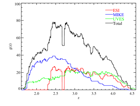
Figure 1: Redshift sensitivity function $g(z)$ for the samples. The sharp feature at $z\simeq 2.7$ is caused by a gap in the ESI data. The upper (black) curve represents the full sample $g(z)$subject to the added constraint that it apply to the data where a SLLS with $N_{\rm HI}$ $>19.3$ cm^-2could be found, with the other curves (blue, red, green) representing the $g(z)$ for the MIKE, ESI, and UVES data samples which comprise the full sample.

3 $N_{\rm HI}$ Analysis

With the survey size defined, we now turn to the SLLS in the survey and discuss the measurement of the $N_{\rm HI}$ for the SLLS, and an estimate of the completeness of the sample.

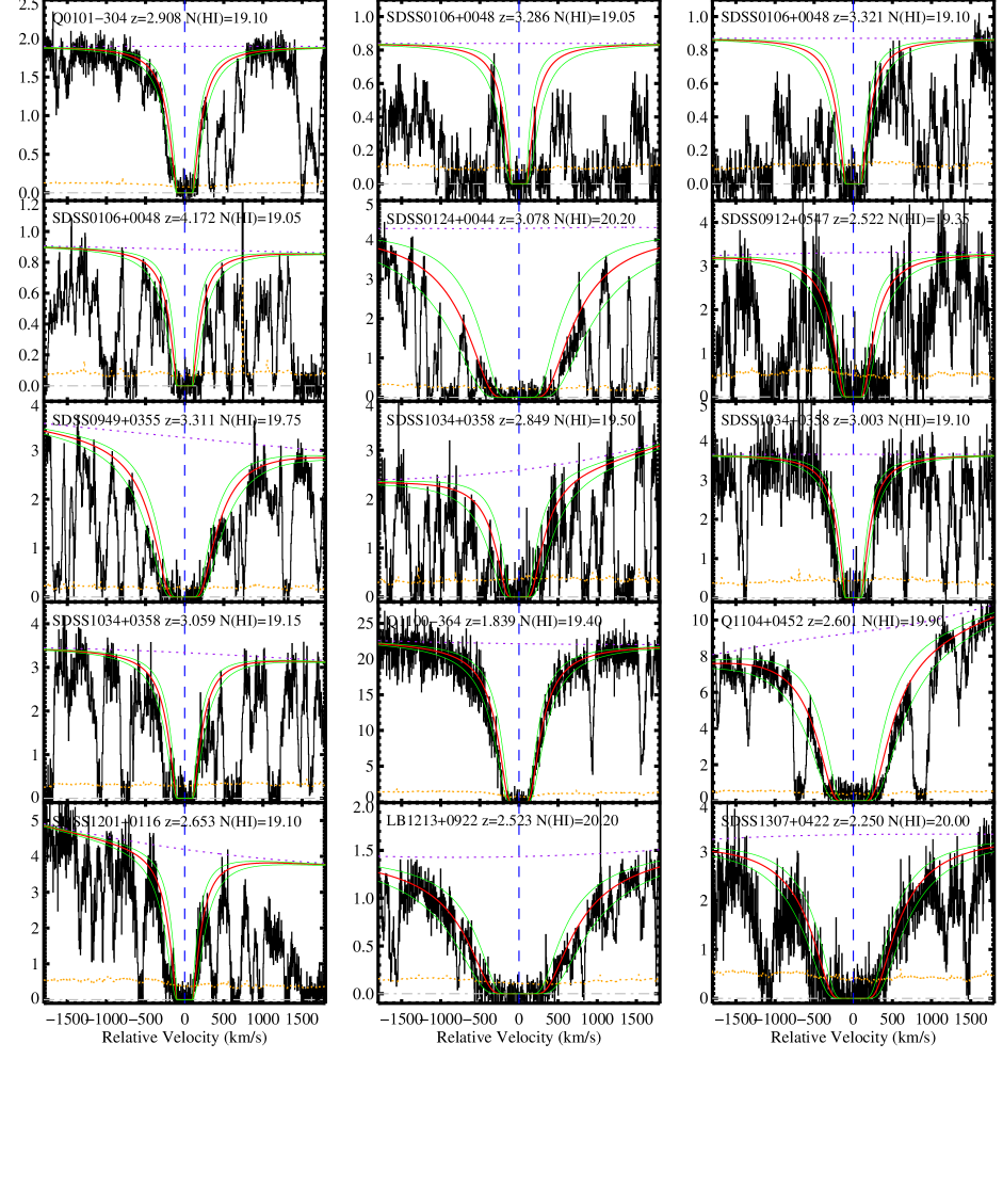
Figure 2: H I Lyman–$\alpha$ transitions for the SLLS in the MIKE sample. The velocity zeropoint is determined from low ionization metal lines whenever possible. Overlaid (in red) are the single component Voigt profile models for the absorption along with the $\pm 1\sigma$ error estimates (in green) on the $N_{\rm HI}$. The horizontal dashed line represents the local continuum level. The vertical dashed line highlights the velocity zeropoint. For each absorber , the QSO name, absorption redshift, and $N_{\rm HI}$ estimate are listed at the top of each panel. In the case of blended SLLS where the individual Ly$\alpha$ lines are separated by more than 300 km s^-1, we show the individual fits (e.g. the SLLS in PKS2000-330).

Fig. 2 – continued

3.1 Identifying SLLS and Measuring $N_{\rm HI}$

To identify the SLLS in our survey, every spectrum from the ESI and MIKE samples was visually inspected for strong absorption in H I Ly$\alpha$. When a candidate SLLS absorber is identified, we first assign a local continuum level to regions approximately 2000 km s^-1 on either side of the absorption. We do not first continuum normalize the data, opting instead to model the absorption and continuum simultaneously. This is done because the damping wings of the Ly$\alpha$ profile may depress the continuum for several tens of Angstroms. It is also necessary to vary the continuum level along with a model to estimate the errors on the $N_{\rm HI}$ values. When the absorption occurs near the QSO emission line features and/or when the redshift of the absorption is high, the assignment of the continuum level is often the dominant source of error. In this work, we assign a minimum value of the error on the $\log N_{HI}$ to be 0.05 dex from continuum level errors alone.

Next, we compared a Voigt profile with $\log N_{HI}$ $=19.0$ cm^-2 at the center of the absorption to determine if it was consistent with at least this amount of atomic hydrogen gas. If metal-line transitions were identified, we use the redshift of the metals to more accurately assign a redshift for the gas. We do not, however, require that metal line absorption be present, because this would introduce an undesirable bias. For most of the absorption systems in our sample, the data cover a wide variety of metal line transitions for each absorber. Common transitions include those of C II, C IV, O I, Si II, Si IV, Al II, and Fe II. In the cases where both low and high ionization metal line transitions are present, we choose to use the redshift given by the low-ion absorption, because these ions more likely trace the atomic hydrogen gas. Finally, for those absorbers meeting our minimum $N_{\rm HI}$ condition, we fit the absorption by stepping through values of $N_{\rm HI}$ until the absorption is well modeled. The Ly$\alpha$ line profile and continuum level were modeled using custom software (the x_fitdla tool within the XIDL package). In the cases when two or more SLLS occur within $\delta v\leq 300$ km s^-1 of each other, the total $N_{\rm HI}$ is reported instead of individual $N_{\rm HI}$ measurements. This is because the individual $N_{\rm HI}$ measurements are highly degenerate and because the gas may physically bound to a single virialized halo.

For each absorber, a number of effects contribute to the error in the $N_{\rm HI}$ value. As mentioned above, we believe that errors in the continuum level contribute at least 0.05 dex to the error. The continuum level error tends to increase with redshift because the amount of absorption from Lyman–$\alpha$ forest increases and one is less certain to identify regions free of absorption. The increase in Lyman–$\alpha$ forest lines also affects the $N_{\rm HI}$ measurement in the damping wings and line core regions of the Ly$\alpha$ line because of enhanced line-blending. Redshift uncertainties were only a minor source of error for each absorber, since nearly every absorption system showed at least one metal-line transition. Finally, the Poisson noise of the data adds additional uncertainty to the fitted value.

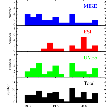
Figure 4: Histograms showing the number of systems detected as a function of $\log N_{HI}$ for the various samples. The upper two panels represent the MIKE and ESI data, which are presented for the first time in this paper. The third panel shows the data from Péroux et al. (2005). The bottom panel shows the full $N_{\rm HI}$ histogram when we combine the three data sets.

In Figures 2 and 3, we show the profile fits and the $\pm 1\sigma$ fits for each LLS in our sample. The values for the $z$, $N_{\rm HI}$, and $\sigma(N_{\rm HI})$ are given in Tables 3 and 4. The LLS listed in these tables do not represent every LLS present in our data. In a number of cases, we removed an SLLS from the sample because the QSO was specifically targeted to study this SLLS. For those SLLS removed, we also remove 1500 km s^-1 of pathlength on either side of the SLLS in the same manner as for the DLA. In total, we have a homogeneous sample of 47 SLLS, of which 17 come from the ESI sample and 30 come from the MIKE sample. Including the UVES sample, there are now a total of 78 SLLS. In Figure 4, we show a histogram of the $N_{\rm HI}$ values for the individual and complete samples.

Table 3: LLS FROM THE MIKE SAMPLE

Name	$z_{abs}$	$\log N_{\rm HI}$	$\sigma(N_{\rm HI})$
Q0101-304	2.908	19.10	0.15
SDSS0106+0048	3.286	19.05	0.25
SDSS0106+0048	3.321	19.10	0.20
SDSS0106+0048	4.172	19.05	0.20
SDSS0124+0044	3.078	20.20	0.20
SDSS0912+0547	2.522	19.35	0.20
SDSS0949+0355	3.311	19.75	0.15
SDSS1034+0358	2.849	19.50	0.25
SDSS1034+0358	3.059	19.15	0.15
SDSS1034+0358	3.003	19.10	0.15
Q1100-264	1.839	19.40	0.15
HS1104+0452	2.601	19.90	0.20
LB1213+0922	2.523	20.20	0.20
SDSS1307+0422	2.250	20.00	0.15
SDSS1402+0146	3.456	19.20	0.30
Q1456-1938	2.351	19.55	0.15
Q1456-1938	2.169	19.75	0.20
SDSS1558-0031	2.630	19.50	0.20
SDSS1621-0042	3.104	19.70	0.20
PKS2000-330	3.188	19.80	0.25
PKS2000-330	3.172	19.80	0.15
PKS2000-330	3.192	19.20	0.25
Q2053-3546	2.350	19.60	0.25
Q2053-3546	2.989	20.10	0.15
Q2053-3546	3.094	19.00	0.15
Q2053-3546	2.333	19.30	0.25
Q2126-158	2.638	19.25	0.15
Q2126-158	2.769	19.20	0.15
HE2314-3405	2.386	19.00	0.20

Table 4: LLS FROM THE ESI SAMPLE

Name	$z_{abs}$	$\log N_{\rm HI}$	$\sigma(N_{\rm HI})$
PX0034+16	3.754	20.05	0.20
SDSS0127-00	2.944	19.80	0.15
PSS0808+52	3.524	19.40	0.20
SDSS0810+4603	3.472	19.90	0.20
SDSS0826+5152	2.862	20.00	0.15
SDSS1004+0018	2.746	19.80	0.20
PSS1248+31	4.075	19.95	0.15
PSS1253-02	3.603	19.50	0.15
SDSS1257-0111	2.918	19.95	0.15
Q1337+11	2.508	20.15	0.15
PSS1432+39	3.994	19.60	0.25
FJ2129+00	2.735	20.10	0.20
PSS2241+1352	3.654	20.20	0.20
SDSS2315+1456	3.135	19.95	0.15
SDSS2315+1456	2.943	19.35	0.20
PSS2323+2758	3.267	19.40	0.20
PSS2323+2758	3.565	19.30	0.20

3.2 Completeness

To gauge the completeness of our $N_{\rm HI}$ analysis we performed a number of tests. Our primary completeness concern is with the detection efficiency at the low H I column density limit of the ESI sample, where the data has lower spectral resolution. At lower resolution, the effects of line blending and continuum level placement tend to wash out the damping wings of $\log N_{HI}$$\simeq 19.0$ Ly$\alpha$ lines. As the column density increases, the equivalent width of the Ly$\alpha$ line also increases and one generally derives a more reliable $N_{\rm HI}$ measurement. Because the MIKE and UVES samples are of higher resolution, the effect at lower column densities is minimized. After experimenting with mock ESI spectra (see below), we chose to limit the ESI analysis to those absorbers with 19.3 cm^-2$\leq$ $\log N_{HI}$$\leq 20.3$ cm^-2. For the MIKE sample, we consider the same range of column densities as in the UVES sample, 19.0 cm^-2$\leq$ $\log N_{HI}$ $\leq 20.3$ cm^-2. Our tests indicate that we have detected all SLLS in these ranges in $N_{\rm HI}$ at a 99% level of completeness.

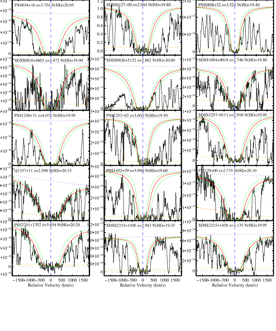
Figure 3: Same as for Figure 2, but for the SLLS in the ESI sample.

Fig. 3 – continued

To verify that the lower bound of $\log N_{HI}$$=19.3$ cm^-2 is appropriate for the ESI sample, we randomly placed mock LLS onto 50 of the ESI spectra. The column densities of these LLS were chosen at random to lie in the range $18.0\leq$$\log N_{HI}$$\leq 20.5$ cm^-2. In all cases, SLLS with $\log N_{HI}$$\geq 19.3$ cm^-2 were identified. Furthermore, the column density fit to these SLLS were within the 2–$\sigma$ error estimates in all cases but one out of fifty. We have also used simulated LLS to address the issue that blending of multiple LLS with $\log N_{HI}$ $\leq 19.3$ cm^-2  could appear as a single absorber with $\log N_{HI}$ $\geq 19.3$ cm^-2 in the ESI sample. As before, we placed mock LLS upon ESI spectra, but in pairs with a random velocity separation $\delta v$ subject to the constraint $\delta v\leq 300$ km s^-1. This constraint matches our velocity separation constraint for the observed SLLS as to whether the $N_{\rm HI}$ is reported as a sum, or as separate systems. The blended, mock LLS absorption was then fit with a single absorption profile, and the $N_{\rm HI}$ compared to the sum of the individual component $N_{\rm HI}$ values. We find that a pair of LLS with $\log N_{HI}$$\leq 18.8\,{\rm cm^{-2}}$ or less can not blend in a manner so as to be fit as an SLLS with $\log N_{HI}$ $\geq 19.3$ cm^-2. However, a blend of a SLLS with $\log N_{HI}$ $\geq 19.3$ cm^-2with a LLS with $\log N_{HI}$ $\sim 19.1$ cm^-2 generally leads to a systematic overestimate of $N_{\rm HI}$. Similarly, a blend of LLS with $\log N_{HI}$$=19.1$ cm^-2 and $\log N_{HI}$ = $18.8$cm^-2 may mimic an SLLS with $\log N_{HI}$ $=19.3$ cm^-2. In essence, this effect leads to a Malmquist bias for the sample at low $N_{\rm HI}$ value. It is not generally possible to directly explore these final two issues without good knowledge of the incidence frequency, clustering properties, and column density distribution of the LLS. Nevertheless, we have some constraints from both the MIKE and UVES samples. Because these samples are of higher resolution, we can often distinguish blended absorption of LLS from a single LLS. Moreover, if two LLS are blended, their metal lines should give some clues that there is blending, provided both LLS have sufficient metallicity. To the extent that we can currently distinguish between blended and unblended LLS, we do not believe that the effect of blended LLS strongly effect our measurements of the $N_{\rm HI}$  but we caution that a larger sample than the one presented here is required to accurately address this issue.

4 Results and Discussion

In this section we discuss a number of results related to the H I frequency distribution of the SLLS. For the majority of the section, we consider two $N_{\rm HI}$ groups driven by the completeness limits of the spectra: (i) $10^{19.0}\,{\rm cm^{-2}}\leq N_{\rm HI}\leq 10^{20.3}\,{\rm cm^{-2}}$ which does not include the ESI sample; and (ii) $10^{19.3}\,{\rm cm^{-2}}\leq N_{\rm HI}\leq 10^{20.3}\,{\rm cm^{-2}}$ which includes all of the samples. The groups cover an integrated absorption pathlength of $\Delta X^{19.0}=329.1$ and $\Delta X^{19.3}=467.7$ respectively. We maintain this division, as opposed to combining the low $N_{\rm HI}$ results from the echelle data with the $N_{\rm HI}\geq 10^{19.3}\,{\rm cm^{-2}}$ analysis, for the following reasons: First, the redshift distribution of the ESI survey (Figure 1) is significantly higher than that of the UVES data and especially the MIKE sample. If there is redshift evolution in $f_{\rm{HI}}(N,X)$, then it would be erroneous to mix the two groups. Indeed, PHW05 find significant evolution int he normalization of $f_{\rm{HI}}(N,X)$ for the damped Ly$\alpha$ systems and one may expect similar evolution in the SLLS population. Second, the division allows us to investigate systematic errors between the various surveys, including the UVES analysis. Finally, we will find it instructive valuable to consider these two $N_{\rm HI}$ groups separately when focusing on the behavior of $f_{\rm{HI}}(N,X)$ near $N_{\rm HI}=10^{19}\,{\rm cm^{-2}}$.

4.1 Power-Law Fits to the $f_{\rm{HI}}(N,X)$ Distribution of the SLLS

In Figures 5 and 6, we show the binned evaluation of $f_{\rm{HI}}(N,X)$ for each of the data-sets, and their combined results. The results are summarized in Table 5. It is evident from the figures that the $f_{\rm{HI}}(N,X)$ distributions can be reasonably modeled by a power-law over the SLLS regime:

$$f_{\rm{HI}}\left(N,X\right)=k_{1}N^{\alpha}\;\;.$$ (3)

We have performed a maximum likelihood analysis on the unbinned $N_{\rm HI}$ distribution to constrain $\alpha$ and set the normalization of $f_{\rm{HI}}(N,X)$. We find $\alpha_{190}=-1.40^{+0.15}_{-0.16}$ and $\alpha_{193}=-1.19^{+0.20}_{-0.21}$ for the combined results of the two groups. Note that the reported errors do not include covariance terms. The results for the individual data samples are all consistent (within $2\sigma$) with the combined results and one another (Table 5).

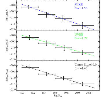
Figure 5: Values for the H I frequency distribution for the SLLS with $19.0\leq$ $\log N_{HI}$ $20.3$cm^-2. Shown separately are the MIKE data presented first here, the UVES sample of Péroux et al. (2003, 2005), and the two samples combined. The four bins span equal size $\Delta$$\log N_{HI}$$=0.3$ except for the last bin which has $\Delta$$\log N_{HI}$$=0.4$. Also shown is the result of a maximum likelihood analysis on the unbinned data for a power-law model of $f_{\rm{HI}}(N,X)$. The power-law index $\alpha$ is given for each sample.

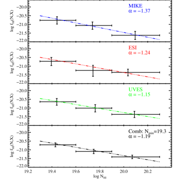
Figure 6: Same as for Figure 5, but with the inclusion of the ESI data, and with the range $19.0\leq$ $\log N_{HI}$ $20.3$ cm^-2, over 3 bins equal in size to the 3 highest H I column density bins in Figure 5. Also shown is the result of a maximum likelihood analysis on the unbinned data for a power-law model of $f_{\rm{HI}}(N,X)$. The power-law index $\alpha$ is given for each sample.

Table 5: $f_{\rm{HI}}(N,X)$ SUMMARY

Sample	$\Delta X$	$\bar{z}$	$m$			log$f_{\rm{HI}}(N,X)$		$\ell_{\rm SLLS}(X)$	$\log k_{1}$	$\alpha_{1}$
				$N\epsilon[19.0,19.3)$	$N\epsilon[19.3,19.6)$	$N\epsilon[19.6,19.9)$	$N\epsilon[19.9,20.3)$
ESI	132.5	3.34	15	…	$-20.72^{+0.22}_{-0.24}$	$-21.24^{+0.30}_{-0.34}$	$-21.36^{+0.19}_{-0.20}$	$0.113^{+0.037}_{-0.029}$	$3.527^{+0.124}_{-0.128}$	$-1.244^{+0.390}_{-0.404}$
MIKE	175.6	2.85	29	$-20.16^{+0.14}_{-0.15}$	$-20.76^{+0.20}_{-0.22}$	$-21.06^{+0.20}_{-0.22}$	$-21.63^{+0.22}_{-0.24}$	$0.165^{+0.037}_{-0.030}$	$9.735^{+0.087}_{-0.088}$	$-1.562^{+0.224}_{-0.240}$
UVES	154.2	3.33	31	$-20.19^{+0.15}_{-0.16}$	$-20.64^{+0.19}_{-0.20}$	$-21.01^{+0.20}_{-0.22}$	$-21.36^{+0.17}_{-0.18}$	$0.201^{+0.043}_{-0.036}$	$4.033^{+0.084}_{-0.085}$	$-1.265^{+0.209}_{-0.216}$
ALL-19.3	467.7	3.08	55	…	$-20.71^{+0.11}_{-0.12}$	$-21.09^{+0.12}_{-0.13}$	$-21.41^{+0.10}_{-0.10}$	$0.118^{+0.018}_{-0.016}$	$2.486^{+0.062}_{-0.062}$	$-1.191^{+0.203}_{-0.206}$
ALL-19.0	329.8	3.10	60	$-20.17^{+0.10}_{-0.10}$	$-20.70^{+0.13}_{-0.14}$	$-21.04^{+0.14}_{-0.15}$	$-21.48^{+0.13}_{-0.14}$	$0.182^{+0.027}_{-0.023}$	$6.716^{+0.059}_{-0.059}$	$-1.405^{+0.153}_{-0.158}$

One notes that the power-law is shallower for the $N_{\rm HI}^{19.3}$ sample than the $N_{\rm HI}^{19.0}$ sample. Although the effect is not statistically significant, we do find the trend is apparent in the independent MIKE and UVES samples. These results suggest that the $f_{\rm{HI}}(N,X)$ distribution is steepening at $N_{\rm HI}<10^{19.3}\,{\rm cm^{-2}}$. We will return to this point in $\S$ 4.4.

4.2 Redshift Evolution

Over the redshift interval $z=2.2$ to 3.5, PHW2005 found that the shape of $f_{\rm{HI}}(N,X)$ for DLA is roughly constant but that the normalization (parameterized by the zeroth moment, $\ell_{\rm{DLA}}$) increases by a factor of approximately two. Similarly, studies of the Ly$\alpha$ forest indicate $\ell(z)^{Ly\alpha}\propto(1+z)^{2.6}$ (Cristiani et al., 1995) at $z\approx 3$ implying $\ell(X)^{Ly\alpha}\propto(1+z)^{2.1}$. One may expect, therefore, that $\ell_{\rm{SLLS}}(X)$ will also increase with redshift over this redshift interval.

In Figure 7, we show the results for $f_{\rm{HI}}(N,X)$ in the two $N_{\rm HI}$ groups, but broken into the redshift regions above (thin line) and below (thick line) $z=3$. A visual inspection of Figure 7 reveals little explicit difference in the shape of $f_{\rm{HI}}(N,X)$ in the two redshift regimes. More formally, a KS test for the two groups returns probabilities of $P_{190}=0.189$ and $P_{193}=0.809$ that the two redshift samples are drawn from the same parent population. Therefore, we contend there is no large redshift evolution in the shape of $f_{\rm{HI}}(N,X)$ for the SLLS over the redshifts considered here.

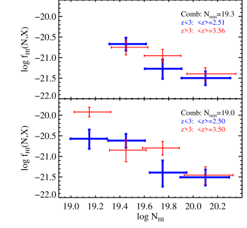
Figure 7: Values for the H I frequency distribution for the SLLS separated into two redshift samples, with the thin symbols corresponding to $z<3$ and the thick symbols corresponding to $z>3$. The upper panel shows the ESI+MIKE+UVES sample and the lower panel the MIKE+UVES sample. The lack of significant change in shape of $f_{\rm{HI}}(N,X)$ for the two redshift bins indicates a lack of strong evolution with redshift in $f_{\rm{HI}}(N,X)$.

Granted that the shape of $f_{\rm{HI}}(N,X)$ for the SLLS is not steeply evolving, we can examine redshift variations in the normalization by examining the zeroth moment

$$\ell_{\rm{SLLS}}(X)=\int\limits_{N_{SLLS}}^{10^{20.3}}f_{\rm{HI}}(N,X)dN$$ (4)

with $N_{SLLS}=10^{19.0}$ or $10^{19.3}\,{\rm cm^{-2}}$. We calculate
$\ell_{\rm{SLLS}}(X)$${}_{(190)}=0.134^{+0.032}_{-0.026}$ and $\ell_{\rm{SLLS}}(X)$${}_{(193)}=0.110^{+0.026}_{-0.021}$ for $z<3$ and $\ell_{\rm{SLLS}}(X)$${}_{(190)}=0.254^{+0.050}_{-0.042}$ and $\ell_{\rm{SLLS}}(X)$${}_{(193)}=0.126^{+0.028}_{-0.023}$ for $z>3$. As is evident from Figure 7 (i.e. focus on the values for the lowest $N_{\rm HI}$ bins), there is no significant redshift evolution in $\ell_{\rm{SLLS}}(X)$ for the $N_{\rm HI}=10^{19.3}\,{\rm cm^{-2}}$ sample. There is, however, an indication of increasing $\ell_{\rm{SLLS}}(X)$ with increasing redshift for the $N_{\rm HI}=10^{19.0}\,{\rm cm^{-2}}$ sample. This result is driven by the lowest $N_{\rm HI}$ bin which we caution is the most sensitive to the effects of line-blending and that such effects are heightened at higher redshift. In summary, there is only tentative evidence for redshift evolution in $\ell_{\rm{SLLS}}(X)$. As noted above, this contradicts the apparent evolution in $\ell(X)$ for the DLA population and the Ly$\alpha$ forest. If confirmed by future studies, perhaps modest evolution in the SLLS population suggests the competing effects of the decrease in the mean density of the universe and a decrease in the intensity of the extragalactic UV background radiation field.

4.3 Is $f_{\rm{HI}}(N,X)$ for the SLLS flatter than the DLA?

There is a significant mismatch in power-law exponents for the Ly$\alpha$ forest ($\alpha_{Ly\alpha}=-1.5$) and the DLA ($\alpha_{DLA}\approx-2$) at $z\approx 3$. This difference predicts that the shape of $f_{\rm{HI}}(N,X)$ change appreciably between these two column densities, i.e., the $f_{\rm{HI}}(N,X)$ distribution of SLLS is flatter than that of the DLA.

The simplest test of this prediction is to measure the power-law index of $f_{\rm{HI}}(N,X)$ in the SLLS regime and compare against its slope near $N_{\rm HI}=10^{20.3}\,{\rm cm^{-2}}$. Both the Gamma function and double power-law fits to $f_{\rm{HI}}(N,X)$ for the SDSS DLA sample indicate $\alpha_{DLA}=-1.9\pm 0.1$ at $N_{\rm HI}<10^{21}\,{\rm cm^{-2}}$ (PHW2005). We compare these values with $\alpha_{SLLS}=-1.19\pm 0.21$ for $\log N_{\rm HI}^{lim}=19.3$ cm^-2and $\alpha_{SLLS}=-1.40\pm 0.15$ for $\log N_{\rm HI}^{lim}=19.0$ cm^-2. The statistical difference in the power-law slope is greater than $2\sigma$ significance but not a full $3\sigma$ result, in terms of the exponents alone.

Figure 8 shows the $f_{\rm{HI}}(N,X)$ distributions for the SLLS and SDSS DLA to a column density of $\log N_{HI}$$=21.5$cm^-2. As before, we show the results for the different SLLS $N_{\rm HI}$ groups separately. Overplotted on the data are the SLLS single power–law fit and the low column density end of the double power-law for the SDSS-DLA (PHW2005). It is apparent that a simple extrapolation of the SDSS-DLA fit significantly overpredicts the frequency of the SLLS, especially at $\log N_{HI}$$<19.7$ cm^-2. We contend, therefore, that the $f_{\rm{HI}}(N,X)$ flattens in slope around the $N_{\rm HI}$ corresponding to the canonical definition for the DLA, $\log N_{HI}$$=20.3$cm^-2. Zheng & Miralda-Escudé (2002) predicted a flattening in $f_{\rm{HI}}(N,X)$ based on photoionization and self-shielding models of isothermal gas profiles in dark matter halos. Although their analysis examined individual halos at a given mass, Zheng (2006, priv. comm.) has convolved their results with a Sheth-Tormen halo mass function (Sheth & Tormen, 1999) and predict $f_{\rm{HI}}(N,X)$ should flatten at $N_{\rm HI}\approx 10^{20}\,{\rm cm^{-2}}$, consistent with our results.

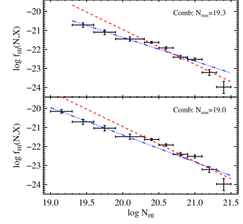
Figure 8: Values for the H I frequency distribution for both the SLLS and the DLA sample of PHW2005. Overplotted are the results for the single power-law for the SLLS from this work (dot-dashed line, power-law index $\alpha=-1.19$ and $\alpha=-1.40$ for the upper and lower plots, respectively), and the low column density end of the double power-law fits to $f_{\rm{HI}}(N,X)$ for the DLA from PHW2005 (dashed line, power law index $alpha=-2.0$). Neither fit describes the full range well, and the $f_{\rm{HI}}(N,X)$ shows a flattening near the canonical DLA definition of $\log N_{HI}$$=20.3$cm^-2.

There are a few cautionary remarks to make regarding Figure 8. First, the shape of the selection functions $g(z)$ for the SLLS and DLA samples do not exactly match because the SLLS database includes a somewhat higher fraction of $z>3$ quasars, and thus a fractionally larger $g(z)$ at those redshifts. Although the mean differs by only $\delta z=0.3$, we note that the comparison is not perfect as we have not considered any evolution in the normalization of $f_{\rm{HI}}(N,X)$ for the SLLS or DLA but have simply plotted the full samples. Another systematic effect is that the SDSS-DLA sample may suffer from a Malmquist bias. Specifically, the statistical and systematic errors (e.g. the effects of line blending) in the $N_{\rm HI}$ values of the DLA are significant and will drive the observed $f_{\rm{HI}}(N,X)$ distribution to a steeper slope. It is possible that this effect explains the marked drop in $f_{\rm{HI}}(N,X)$ at $N_{\rm HI}=10^{20.7}\,{\rm cm^{-2}}$ in Figure 8. We intend to address this issue directly with follow-up, higher resolution observations of a large sample of SDSS-DLA with $N_{\rm HI}\approx 10^{20.3}\,{\rm cm^{-2}}$. If there is a substantial Malmquist bias in the DLA sample, then the decrease in the slope of $f_{\rm{HI}}(N,X)$ would be more gradual than that suggested by Figure 8.

4.4 Is There an Inflection in $f_{\rm{HI}}(N,X)$ within the SLLS Range?

While the mismatch between the DLA and the Ly$\alpha$ forest in the power-law description of their $f_{\rm{HI}}(N,X)$ distributions suggests that $f_{\rm{HI}}(N,X)$ for the LLS will show intermediate values ($\alpha\approx-1.7$), the observed incidence of LLS reveals a different result. As PHW2005 discussed, a simple spline interpolation of the DLA and Ly$\alpha$ forest $f_{\rm{HI}}(N,X)$ distributions through the LLS regimes predicts over an order of magnitude more LLS than observed per $\Delta X$. PHW2005 argued, therefore, that the $f_{\rm{HI}}(N,X)$ distribution for the LLS must exhibit an inflection as evidenced by $d\log f/d\log N>-1.5$. Zheng & Miralda-Escudé (2002) have also predicted that there should be an inflection in $f_{\rm{HI}}(N,X)$ in the SLLS regime for galaxies exposed to an ionizing radiation field. It is worth investigating with our data-set whether evidence exists for just such an inflection.

The simplest approach is to examine whether $d\log f/d\log N>-1.5$ in the LLS regime. Regarding our results on the SLLS, we find that $d\log f/d\log N>-1.5$ for both the $\log N_{\rm HI}^{lim}=19.0$ cm^-2and $\log N_{\rm HI}^{lim}=19.3$ cm^-2groups (Table 5). The differences, however, have less than $2\sigma$ significance. Using only the current data-set and the distribution of DLAs, we do not report the existence of an inflection in $f_{\rm{HI}}(N,X)$ within the SLLS regime.

4.4.1 Constraints from lower $N_{\rm HI}$ LLS

In order to pursue the question further, we introduce two new observational constraints on the LLS. The statistical significance for the SLLS alone is limited by the combination of sample size and observed baseline in $\log N_{HI}$. We cannot arbitrarily increase the sample size, but we are able to introduce new constraints which are sensitive to lower column density LLS. The number density of optically thick LLS has been well constrained by many studies. For our purposes here, we apply the constraint at redshift $z=3$ of $\ell(X)_{LLS}=0.7\pm 0.1$ (Sargent, Steidel & Boksenberg, 1989; Storrie-Lombardi et al., 1994; Péroux et al., 2003). We also use a measure of the incidence of optically thin partial Lyman Limit Systems (PLLS) from Burles (1997), who found 12 systems with mean redshift at $z=3$ with 17.2 cm^-2$<\log N_{HI}<$ 17.8 cm^-2 over a redshift path of $\Delta z_{PLLS}=59.07$ and absorption path of $\Delta X_{PLLS}=16.63$. This gives $\ell(X)_{PLLS}=0.20\pm 0.06$.

4.4.2 The observable distribution function ${\mathcal{O}}(N,X)$

In order to facilitate the analysis and interpretation of the distribution over the full range of LLS and DLAs, we introduce a function called the observable distribution function of H I:

$${\mathcal{O}}(N,X)=\frac{m}{\Delta\log N\Delta X}\;=\frac{\ell(X)}{\Delta\log N}\;,$$ (5)

where m is the number of systems observed over an absorption path, $\Delta X$, and a column density range $\Delta\log N$. This is simply the frequency distribution function in logarithmic column density bins and is related to the classic distribution by:

$${\mathcal{O}}(N,X)\,d{\rm log}N=f(N,X)dN\,,\\ {\mathcal{O}}(N,X)=f(N,X)\,N\,\ln(10)\;.$$ (6)

The observable distribution has a few nice features. It is unitless, and gives the direct number of systems observed over a specified bin in logarithmic column density (almost all studies of H I absorption show and analyze the data in bins of constant width in $\log N_{HI}$). It also removes one factor of column density from the steep slope in the frequency distribution, which enables better assessments of change in slopes, as well as smaller effects from the rapid change in the distribution over bins of large size.

4.4.3 ${\mathcal{O}}(N,X)$for the LLS and the DLA

In Figure 9, we show the observational constraints on ${\mathcal{O}}(N,X)$ from the present sample of SLLS and the DLA from PHW2005. In addition, we show an observational constraint on the abundance of partial Lyman limits at $z=3$, ${\mathcal{O}}_{PLLS}=0.42\pm 0.13$, corresponding to the column density interval (17.2 cm^-2$<\log N_{HI}<$ 17.8 cm^-2; Burles, 1997).

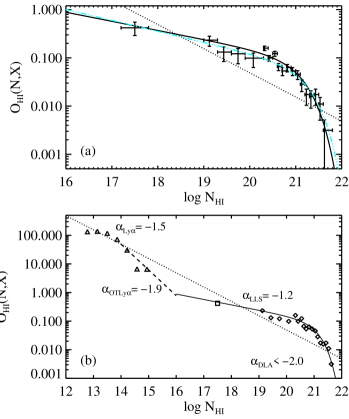
Figure 9: a) Values for the observable distribution function for the entire range of H I absorbers which are optically thick at the Lyman limit. The solid line is a best fit 3 parameter function (assuming Gaussian statistics) of the data which include the SLLS presented here, the DLA from PHW2005, and a bin which contains the constraint on the number of partial LLS. The dot-dashed line shows the best fit after removing the two outlying bins from the PHW sample. Also shown (dotted line) is the ${\mathcal{O}}(N,X)$ for the Lyman–$\alpha$ forest. b) Same as a), but extended to include the Lyman–$\alpha$ forest results of (Kirkman & Tytler, 1997), which are shown as the triangles. The constraint from the number of partial LLS is displayed by the square. Overlaid are the values for the power-law slope $\alpha$ for the $N_{\rm HI}$ regions: $\alpha_{Ly\alpha}$ corresponding to the optically thin Lyman–$\alpha$ forest with $12.1<$ $\log N_{HI}$ $<14$, $\alpha_{OTLy\alpha}$ corresponding to the optically thick Lyman–$\alpha$ forest with $14<$ $\log N_{HI}$ $<16$, $\alpha_{LLS}$ corresponding to $16<$ $\log N_{HI}$$<20.3$, and $\alpha_{DLA}$ corresponding to $\log N_{\rm HI}=20.3-21.3$, to highlight the observed and predicted changes in the logarithmic slope of $f_{\rm{HI}}(N,X)$.

We fit a simple analytic function to the combined set of ALL-19.0 SLLS (Table 5), the PHW2005 DLA sample for $\log N_{HI}$$>20.3$ cm^-2, as well as the two additional LLS constraints described above. We fit a three parameter model expressed as:

$${\rm log}\,{\mathcal{O}}(N,X)=a+b*(\log N_{HI}-19)-10^{\log N_{HI}-c}$$ (7)

This parameterized form can be recast into a more familiar $\Gamma$-distribution (e.g. Pei & Fall, 1995; Péroux et al., 2003):

$${\mathcal{O}}(N,X)={\mathcal{O}_{0}}\,\left(\frac{N_{\rm HI}}{N_{*}}\right)^{\alpha+1}\,e^{-\frac{N_{\rm HI}}{N_{*}}}$$ (8)

where ${\rm log}\,N_{*}=c-0.3622,\;\;{\rm log}\,{\mathcal{O}_{0}}=b\,{\rm log}\,N_{*}+(a-19b),\;\;\alpha=b-1$.

We show the best fit function to the binned data assuming Gaussian statistics as the solid line in Figure 9, parameterized by $(a,b,c)=(-0.621,-0.189,21.51)$, which gives a reduced $\chi^{2}$ for 17 degrees of freedom (dof), $\chi_{\nu}^{2}=1.86$. We assess the dependence of the fitting on the included data-sets, by sequentially removing constraints. If we do not include the constraint on the total number of optically thick Lyman limits, the best fit parameters are virtually unchanged, and the fitted parameters above give a predicted number of optically thick Lyman limits of: $\ell(X)^{fit}_{LLS}=0.68$. The two outliers in the above fit are the DLA points centered near bins of $\log N_{HI}$= 20.3 and 20.6 cm^-2. If we drop the first of these points, we find $(-0.660,-0.198,21.56)$ and $\chi_{\nu}^{2}=1.24$ for 15 dof. Dropping both DLA bins gives an acceptable fit, with $(-0.677,-0.227,21.63)$ and $\chi_{\nu}^{2}=0.552$ for 14 dof. The last fit is shown as a dashed-dotted line in Figure 9.

The fits show that the ${\mathcal{O}}(N,X)$ slope in the SLLS region falls between $-0.227<b<-0.189$ (recall $\alpha=b-1$). We also find that the HI cutoff scale is between $21.51<c<21.63$ which matches the results of PHW2005 and Péroux et al. (2003). All the fits produce a reasonable number of optically thick Lyman limit systems: $0.61<\ell_{\rm{LLS}}(X)<0.68$.

4.4.4 Are the SLLS a distinct population?

Finally, we present another moment of the $N_{\rm HI}$ distribution, $N_{\rm HI}$${\mathcal{O}}(N,X)$, in Figure 10. This represents the total H I column density per unit logarithmic column density per unit absorption path. The SLLS and DLA data points and the first analytic fit (to the entire data set) is shown. The data are relatively flat from $N_{\rm HI}=10^{20.3}\,{\rm cm^{-2}}$ to $10^{21.5}\,{\rm cm^{-2}}$ with the functional form peaking at $logN_{\rm HI}=21.1$. It is evident that absorbers with $N_{\rm HI}\approx 10^{21}\,{\rm cm^{-2}}$ dominate the mass density of H I in the universe. Consider a comparison of the SLLS and DLA. Whereas the damped Ly$\alpha$ systems with $20.3<\log N_{\rm HI}<21.5$ dominate the mass density with roughly equal contribution per $\Delta\log N$, the SLLS lie distinctly below, with the absorbers at $N_{\rm HI}=10^{19}$cm^-2 adding a negligible portion and the full SLLS range in $N_{\rm HI}$ contributing only $\approx 15\%$ to the total mass density. We note that Zwaan et al. (2005) obtain a very similar shape for $N_{\rm HI}$${\mathcal{O}}(N,X)$at $z=0$. Again, this behavior is likely related to the fact that the majority of SLLS are highly ionized. The results in Figure 10 lends further support to the concept that the SLLS absorbers are a distinct population from the damped Ly$\alpha$ systems.

Figure 10: Values for $N_{\rm HI}$${\mathcal{O}}(N,X)$, the first moment of the observable distribution function over the SLLS and DLA range. The data give the relative contributions to the cosmic density of hydrogen atoms per unit $\log N_{HI}$ at $z\sim 3$, and show that DLA with $\log N_{HI}$= 20.3 – 21.5 overwhelmingly dominate the H I mass density, with the SLLS contributing only $\approx 15\%$ to the total.

4.5 Implications for lower $N_{\rm HI}$

Armed with a description for the full range of H I column densities which are optically thick at the Lyman limit, we now wish to extend our analysis downward in $N_{\rm HI}$ to the Lyman–$\alpha$ forest. Although a more thorough analysis is required to fully assess the statistically acceptable distributions over such a large range in $\log N_{HI}$, we can clearly show that slopes in the SLLS region as steep as $\alpha=-1.5$ are unacceptable. In Figure 9b, we overplot the extrapolation of the best fit observable distribution of low column density Lyman-$\alpha$ absorbers ($12.1<\log N_{HI}<14$) as a dotted line with a slope of $b=-0.5$ (i.e., $f_{\rm{HI}}(N,X)$$\propto N^{-1.5}$; Kirkman & Tytler, 1997). Although the extrapolation has uncertainties related to the normalization and completeness, it does highlight the overprediction of SLLS based on a simple power-law extrapolation from lower column density studies. Even if we allowed for freedom in normalization, it is clear that in no region except near $\log N_{HI}$= 20.5 cm^-2 is $\alpha=-1.5$ a good description of the high $\log N_{HI}$ distribution. A subset of the data which were used constrain the fit to Lyman-$\alpha$ absorbers is shown in the lower panel of Figure 9 as triangles. A gamma function with low-end slope of $\alpha=-1.2$ is a good fit to the high density data sets of LLS and DLAs. But the extrapolation of the low end slope to the regime of the Lyman-$\alpha$ absorbers underpredicts the observed numbers by almost a factor of 100!

In order to reconcile the data presented here, together with the DLAs, LLSs and the Lyman-$\alpha$ absorbers, the full distribution function must contain at least three changes in logarithmic slope of the frequency distribution (or inflections, $d^{2}f/dN^{2}=0$), as previously argued (in part) by Bechtold (1987) and Petitjean et al. (1993). The first inflection is seen in the change between the DLA distribution and SLLS. This is required if one includes constraints from the LLS and the PLLS and demands constant slopes down to these column densities. There must then be at least two more changes in the logarithmic slopes, one to account for the much higher number of Lyman-$\alpha$ absorbers, and the second to finally merge back to the Lyman-$\alpha$ slope with $\alpha=-1.5$. We present one such solution with a dotted line bridging the gap between $\log N_{HI}$= 14 cm^-2 and $\log N_{HI}$= 16 cm^-2 with a frequency slope of $\alpha=-1.9$. The Lyman-$\alpha$ absorbers are claimed to have a single power law slope over two decades of $N_{\rm HI}$(12.5cm^-2$<\log N_{HI}<$14.5cm^-2), and are classified as a single population. In comparison, the absorbers spanning 17cm^-2$<\log N_{HI}<$20cm^-2, over three decades of $N_{\rm HI}$, are well described by a single power law slope of $\alpha=-1.2$ and also could be classified as a single population by applying the same argument.

5 Concluding Remarks

The SLLS results presented in this paper motivate several avenues of future exploration. First, we must extend the survey downward in LLS H I column density. An improved constraint on the number of optically thick LLSs would significantly tighten the constraint on the low-end slope of the SLLS distribution. Second, a large sample of higher H I column density Lyman–$\alpha$ forest data is needed. Specifically, a large sample of Lyman–$\alpha$ forest with $14.5\leq$ $\log N_{HI}$  $\leq 16.5$ cm^-2  directly tests the predicted shape of the H Idistribution. Finally, one must pursue detailed ionization studies of the LLS to fully assess their baryonic mass, metallicity, etc. Our survey will provide the data-set required for just such studies.

References

- Adelman-McCarthy et al. (2006) Adelman-McCarthy, J. K. et al. 2006, ApJS, 162, 38.
- Bahcall & Peebles (1969) Bahcall, J. N. and Peebles, P. J. E. 1969, ApJ, 156, L7+.
- Bechtold (1987) Bechtold, J. 1987, in High Redshift and Primeval Galaxies, ed. J. Bergeron, D. Kunth, B. Rocca-Volmerange, and J. Tran Thanh van, 397.
- Bennett et al. (2003) Bennett, C. L. et al. 2003, ApJS, 148, 1.
- Bernstein et al. (2003) Bernstein, R. et al. 2003, in Instrument Design and Performance for Optical/Infrared Ground-based Telescopes. Edited by Iye, Masanori; Moorwood, Alan F. M. Proceedings of the SPIE, Volume 4841, pp. 1694-1704 (2003)., 1694.
- Bouché, Lehnert & Péroux (2006) Bouché, N., Lehnert, M. D., and Péroux, C. 2006, MNRAS, 367, L16.
- Burles, Bernstein & Prochaska (2006) Burles, S., Bernstein, R., and Prochaska, J. 2006, In prep.
- Burles (1997) Burles, S. M. 1997, Ph.D. Thesis.
- Burles & Tytler (1998) Burles, S. and Tytler, D. 1998, ApJ, 507, 732.
- Cristiani et al. (1995) Cristiani, S. et al. 1995, MNRAS, 273, 1016.
- Croft et al. (2002) Croft, R. A. C. et al. 2002, ApJ, 581, 20.
- Dekker et al. (2000) Dekker, H. et al. 2000, in Proc. SPIE Vol. 4008, p. 534-545, Optical and IR Telescope Instrumentation and Detectors, Masanori Iye; Alan F. Moorwood; Eds., ed. M. Iye and A. F. Moorwood, 534.
- Dessauges-Zavadsky et al. (2003) Dessauges-Zavadsky, M. et al. 2003, MNRAS, 345, 447.
- Kim et al. (2002) Kim, T.-S. et al. 2002, MNRAS, 335, 555.
- Kirkman & Tytler (1997) Kirkman, D. and Tytler, D. 1997, ApJ, 484, 672.
- Kirkman et al. (2003) Kirkman, D. et al. 2003, ApJS, 149, 1.
- Lanzetta (1991) Lanzetta, K. M. 1991, ApJ, 375, 1.
- Lanzetta (1993) Lanzetta, K. M. 1993, in ASSL Vol. 188: The Environment and Evolution of Galaxies, ed. J. M. Shull and H. A. Thronson, 237.
- McDonald et al. (2005) McDonald, P. et al. 2005, ApJ, 635, 761.
- Pei & Fall (1995) Pei, Y. C. and Fall, S. M. 1995, ApJ, 454, 69.
- Péroux et al. (2003) Péroux, C. et al. 2003a, MNRAS, 345, 480.
- Péroux et al. (2005) Péroux, C. et al. 2005, MNRAS, 363, 479.
- Péroux et al. (2006) Péroux, C. et al. 2006, A&A, 450, 53.
- Péroux et al. (2003) Péroux, C. et al. 2003b, MNRAS, 346, 1103.
- Petitjean et al. (1993) Petitjean, P. et al. 1993, MNRAS, 262, 499.
- Prochaska (1999) Prochaska, J. X. 1999, ApJ, 511, L71.
- Prochaska et al. (2003) Prochaska, J. X. et al. 2003, ApJS, 147, 227.
- Prochaska & Herbert-Fort (2004) Prochaska, J. X. and Herbert-Fort, S. 2004, PASP, 116, 622.
- Prochaska et al. (2006) Prochaska, J. X. et al. 2006, ApJ, 648, L97.
- Prochaska & Wolfe (1999) Prochaska, J. X. and Wolfe, A. M. 1999, ApJS, 121, 369.
- Sargent, Steidel & Boksenberg (1989) Sargent, W. L. W., Steidel, C. C., and Boksenberg, A. 1989, ApJS, 69, 703.
- Sheinis et al. (2002) Sheinis, A. I. et al. 2002, PASP, 114, 851.
- Sheth & Tormen (1999) Sheth, R. K. & Tormen, G. 1999, MNRAS, 308, 119.
- Steidel (1990) Steidel, C. C. 1990, ApJS, 74, 37.
- Stengler-Larrea et al. (1995) Stengler-Larrea, E. A. et al. 1995, ApJ, 444, 64.
- Storrie-Lombardi et al. (1994) Storrie-Lombardi, L. J. et al. 1994, ApJ, 427, L13.
- Tytler (1982) Tytler, D. 1982, Nature, 298, 427.
- Tytler et al. (2004) Tytler, D. et al. 2004, ApJ, 617, 1.
- Viegas (1995) Viegas, S. M. 1995, MNRAS, 276, 268.
- Wolfe, Gawiser & Prochaska (2005) Wolfe, A. M., Gawiser, E., and Prochaska, J. X. 2005, ARA&A, 43, 861.
- Zheng & Miralda-Escudé (2002) Zheng, Z. and Miralda-Escudé, J. 2002, ApJ, 568, L71.
- Zwaan et al. (2005) Zwaan, M. A. et al. 2005, MNRAS, 364, 1467.