Simulations of Electron Acceleration at Collisionless Shocks: The Effects of Surface Fluctuations

Abstract

Energetic electrons are a common feature of interplanetary shocks and planetary bow shocks, and they are invoked as a key component of models of nonthermal radio emission, such as solar radio bursts. A simulation study is carried out of electron acceleration for high Mach number, quasi-perpendicular shocks, typical of the shocks in the solar wind. Two dimensional self-consistent hybrid shock simulations provide the electric and magnetic fields in which test particle electrons are followed. A range of different shock types, shock normal angles, and injection energies are studied. When the Mach number is low, or the simulation configuration suppresses fluctuations along the magnetic field direction, the results agree with theory assuming magnetic moment conserving reflection (or Fast Fermi acceleration), with electron energy gains of a factor only $2-3$. For high Mach number, with a realistic simulation configuration, the shock front has a dynamic rippled character. The corresponding electron energization is radically different: Energy spectra display: (1) considerably higher maximum energies than Fast Fermi acceleration; (2) a plateau, or shallow sloped region, at intermediate energies $2-5$ times the injection energy; (3) power law fall off with increasing energy, for both upstream and downstream particles, with a slope decreasing as the shock normal angle approaches perpendicular; (4) sustained flux levels over a broader region of shock normal angle than for adiabatic reflection. All these features are in good qualitative agreement with observations, and show that dynamic structure in the shock surface at ion scales produces effective scattering and can be responsible for making high Mach number shocks effective sites for electron acceleration.

1 Introduction

Collisionless shocks are a key component of many astrophysical systems, since they act as sites of particle acceleration and thermalization, converting upstream bulk flow energy into downstream thermal energy, and at the same time transferring energy to a small fraction of energetic particles. The internal structure of a collisionless shock determines the thermalization process, and a controlling factor is the magnetic geometry of the shock, usually described by the angle $\theta_{Bn}$ between the shock normal and the upstream magnetic field direction. Quasi-parallel ($\theta_{Bn}<45^{\circ}$) and quasi-perpendicular ($\theta_{Bn}>45^{\circ}$) shocks have very different internal structure, different thermalization processes, and are also predominantly associated with different acceleration mechanisms: diffusive (Fermi) acceleration and shock drift acceleration (SDA), respectively.

For quasi-perpendicular shocks in the heliosphere, the internal structure is well established, both observationally and with simulations (e.g., Burgess, 1995). At sufficiently high Mach numbers (supercritical) ion reflection is required to provide the required downstream heating. Specularly reflected ions gyrate in front of the shock (due to the quasi-perpendicular geometry) forming a “foot” in the magnetic field and density ahead of the main ramp. The reflected ions, as they transit downstream, are also responsible for an overshoot-undershoot structure immediately after the ramp. The overshoot means that the magnetic field magnitude peaks at a larger value than the simple expectation from the shock conservation relations for a high Mach number perpendicular shock. At subcritical Mach numbers, there is little or no ion reflection, and dispersion and/or dissipation provides the limiting process against nonlinear steepening.

Energetic electrons up to 100 keV are commonly observed at interplanetary shocks and at planetary bow shocks. They are also invoked in mechanisms of radio emission in the solar corona and the interplanetary medium. Tsurutani & Lin (1985) reported observations of interplanetary shocks with associated spikes and step-like increases in electron fluxes in the energy range $2-20$ keV. The largest events were at shocks with $\theta_{Bn}\stackrel{{\scriptstyle<}}{{\sim}}70^{\circ}$ and with high (relative to the data set) shock Mach number. Some shock crossings had no accelerated electron signature, and these were those with low Mach number and small $\theta_{Bn}$. Higher energy electrons, up to at least 100 keV can sometimes be associated with interplanetary shocks (e.g., Simnett et al., 2005).

Anderson et al. (1979) observed electrons up to 100 keV ahead of the Earth’s bow shock, in a thin sheet just downstream of the tangent surface formed from the solar wind field lines touching the curved bow shock surface. It was found that the most energetic electrons ( $>5.3$ keV) originated on the bow shock where $\theta_{Bn}>85.5^{\circ}$, i.e., closest to the magnetic tangent point. It was clear that the most energetic electrons were associated with the quasi-perpendicular shock, indeed the near-perpendicular shock. These observations led to the suggestion that reflection of incident electrons was important to the acceleration process. Holman & Pesses (1983) outlined a mechanism for type II solar radio bursts in which upstream electrons were reflected and energized by shock drift acceleration (SDA).

Based on the idea of reflection at the quasi-perpendicular shock by conservation of magnetic moment, Wu (1984) and Leroy & Mangeney (1984) developed an analytic model for electron acceleration out of the thermal distribution. The theory was developed for a planar, time-steady shock with scatter-free propagation for the electrons. The de Hoffman-Teller frame (HTF) is the shock frame in which the upstream flow is directed along the magnetic field so there is zero motional electric field. In the HTF particles conserve their energy and magnetic moment if their propagation is scatter-free and the scale lengths and time scales are long compared to their cyclotron motion. Reflection is described by magnetic mirroring (or adiabatic reflection), with some additional effects at low energy due to the cross-shock potential. In the normal incidence frame (NIF) the particles drift in the gradient of the magnetic field along the motional electric field direction, and thus gain energy. Krauss-Varban & Wu (1989) have shown the equivalence of the HTF and NIF descriptions of the energization process. Since scatter-free propagation is assumed, the reflected distribution function and moments can be calculated by Liouville mapping from the incident distribution. An electron which is reflected has to satisfy the conditions that its magnetic moment is appropriate for magnetic mirroring, and that its parallel velocity after reflection is high enough to escape the shock (i.e., in the HTF its parallel velocity is directed upstream). As $\theta_{Bn}$ approaches 90^∘ the frame transformation velocity from NIF to HTF increases, and the portion of the incident distribution that will mirror, and have an upstream directed velocity in the HTF, has an increasingly high energy in the incident flow frame. Thus, the reflected accelerated density depends strongly on the form of the incident distribution above thermal energies. This produces a paradox: acceleration due to magnetic mirroring will give the highest energies for shocks closest to perpendicular, but the same shocks produce the lowest reflected fraction. This situation is ameliorated by using either a core plus halo or kappa distribution upstream, as is typical for solar wind electrons (e.g., Fitzenreiter et al., 1990).

The results of adiabatic reflection theory have been tested, and broadly confirmed for energies up to at least $10-20$ keV, using a combination of test particle integration and self-consistent, one-dimensional hybrid simulation of the shock fields (Krauss-Varban et al., 1989). The use of self-consistent shock simulations removes the need to make model assumptions about the magnetic field and electric potential profiles. It was also realized that, in the scatter free approximation, the electrons could travel a long distance along the magnetic field direction during their reflection process, and thus shock curvature would become important. Modeling of a curved shock was carried out which revealed a flux focusing effect, so that particles entering at $\theta_{Bn}$ close to $90^{\circ}$ drift and exit at a slightly lower value (Krauss-Varban & Burgess, 1991). This latter result is again for the case of scatter-free motion.

The effects of a curved shock, with finite width, were also investigated by Vandas (1995) using a model shock profile. This work was extended to include comparisons between modeled and observed upstream anisotropies and energy spectra at the Earth’s bow shock (Vandas, 2001). The assumptions of magnetic moment conserving reflection and scatter-free Liouville mapping make it possible to construct the distribution function of reflected electrons throughout the foreshock, i.e., the region ahead of, and magnetically connected to the bow shock (Cairns, 1987). This has been used for two purposes: Firstly, in order to make comparisons with observations of low energy electrons in the terrestrial foreshock (Fitzenreiter et al., 1990), and, secondly, as a component in models of foreshock radio emission. For example, Kuncic et al. (2004) describe a quantitative model of fundamental and second harmonic emission in the Earth’s foreshock, using electron beam properties derived from adiabatic reflection of electrons out of the solar wind distribution. Knock et al. (2003) constructed a similar model to explain interplanetary Type II radio bursts, based on acceleration at a large scale “ripple” on the surface of an interplanetary shock. Electron acceleration in a “wavy” shock front was also modeled by Vandas & Karlický (2000) to explain solar Type II radio bursts.

Adiabiatic reflection theory has several positive aspects: It produces qualitative agreement with observations in terms of the origin and energies of accelerated electrons. Furthermore, observations at lower energies ($<1$ keV) often show loss-cone features in agreement with magnetic mirroring (e.g., Fitzenreiter et al., 1990). However, for the more energetic electrons, the theory fails to explain the observed energy spectra and anisotropies at the shock (Vandas, 2001). Observations at the Earth’s bow shock in the energy range $1-20$ keV show that the suprathermal electron flux appears as an inverse power law (with exponent $3-4$ for the phase space density) which emerges smoothly from the downstream thermal distribution, with fluxes peaking just downstream, and the highest energies ($>5$ keV) appearing at the shock overshoot where the distribution is nearly isotropic (Gosling et al., 1989). The backstreaming (so-called reflected) component is seen in the shock ramp, and this was interpreted as escaping particles which have been energized at, and just downstream of the shock.

The observation of a high energy power law tail for the shock accelerated electrons, both upstream and downstream, and small downstream anisotropy, are difficult to explain in the context of adiabatic reflection, which, as in SDA, is a single encounter process. Vandas (2001) concluded that some other process, such as pitch angle scattering, must modify the reflection process, in order to explain observations. Modeling of the effects of such scattering in a curved shock was carried out by Krauss-Varban (1994), although the scattering was introduced in an ad-hoc manner.

So far we have concentrated on the idea that the acceleration is due to the shock acting as a moving magnetic mirror. However, electron acceleration is also possible by a high level of turbulence within the shock layer. For example, Cargill & Papadopoulos (1988) investigated the possibility that a Bunemann instability of the reflected ion beam at high Mach numbers can lead to strong electron heating. Electron heating and (via formation of nonthermal tails) acceleration have been studied with full particle (kinetic ion and electron) plasma shock simulations (e.g. Bessho & Ohsawa, 2002; Lembège & Savoini, 2002). The formation of an electron foreshock at a curved shock has been studied with a full particle simulation (Savoini & Lembège, 2001). Schmitz et al. (2002) presented full particle simulations where accelerated electrons interacted with waves in the foot of the shock, and could be trapped in electron phase space hole structures, thereafter they interacted with the shock in a manner approximately conserving magnetic moment. Although such full particle PIC simulations give an insight into the various physical interactions, they are hampered by computational constraints which mean the use of non-realistic ion-electron mass and ion-electron plasma frequency ratios. It has been shown that using a low value for the mass ratio in such simulations can lead to behavior which is not seen when the correct value is used (Scholer et al., 2003). Thus, there are some questions about the applicability of the results of such simulations to interplanetary and planetary shocks; their results may be more applicable to high Mach number relativistic shocks.

The work in this paper starts from the idea that the quasi-perpendicular shock acts as a magnetic mirror, and that, for initial energies just above thermal, electron scale fluctuations can be neglected, so that the hybrid simulation method is appropriate (Krauss-Varban et al., 1989). It is shown, using a combination of self-consistent and test particle simulations, that the inclusion of structure along the magnetic field lines (and across the surface of the shock) produces scattering within the shock layer which fundamentally changes the resulting upstream and downstream electron distributions. In particular, we find that power law energy spectra can be produced both downstream as well as upstream, and that the range of $\theta_{Bn}$ over which acceleration is effective broadens, so the overall efficiency of the process increases.

The paper is organized as follows: Section 2 describes both the hybrid and test particle parts of the simulations; Section 3.1 demonstrates the types of shock structure that are found in the hybrid simulations; Section 3.2 gives the resulting energetic electron spectra; finally, Section 4 summarizes and briefly discusses the results.

2 Simulations

The method we use is similar to earlier work (Krauss-Varban et al., 1989). The major difference is that a spatially two dimensional hybrid simulation is used, rather than the one dimensional simulation used in earlier work. Two dimensional hybrid simulations of the quasi-perpendicular shock were first carried out by Winske & Quest (1988), who showed the presence of large amplitude fluctuations in the field and density at the shock transition. These fluctuations of the surface of the shock have been analyzed in terms of turbulent ripples (Lowe & Burgess, 2003).

The simulation is carried out in two stages. First, the electric and magnetic fields for the shock transition are generated using a hybrid plasma simulation. Data for all time steps and grid points is stored. The hybrid plasma simulation models the electron response as a fluid. Ions are modeled using simulation macroparticles as in the standard PIC method. The hybrid method has a number of advantages suited to the collisionless shock problem. Ion kinetic effects are retained, including ion reflection which is crucial to correct modeling of the shock structure. On the other hand, the fluid electron response means that relatively long times and large spatial domains can be simulated. This is important for the interaction of electrons with the shock, since, at the energies and Mach number considered here, they convect into the shock at the bulk flow speed. At a supercritical shock the convection time of a field line through the shock structure is of the order of the ion cyclotron time, since the foot structure scales with the Larmor radius of the reflected ions. Thus to study properly the process of electron energization the shock fields must be simulated on ion time scales. The electron fluid response is also appropriate to planetary bow shocks and interplanetary shocks, where strong electron heating is only rarely observed.

The second stage of the simulation consists of integrating the equations of motion of an ensemble of test particle electrons in the time varying fields obtained from the hybrid simulation. Careful interpolation of the fields in time and space is required to ensure accuracy, otherwise artificial scattering of the test particles may be introduced. The initial conditions used in this work are to follow a shell of mono-energetic electrons released upstream, until they reach either specified upstream or downstream collection points.

We now give details of the simulation. The hybrid simulation models the plasma with macro-particle ions (protons) and a massless, charge neutralizing electron fluid with an adiabatic equation of state. The simulation method is described in Matthews (1994). Distances are normalized to the ion inertial length $c/\omega_{pi}$, time to the inverse cyclotron frequency $\Omega_{ci}^{-1}$, velocity to the Alfvén speed $v_{A}$; all normalizations use upstream values. The magnetic field is normalized to its upstream value, $B_{0}$.

The shock is launched by the injection method, whereby plasma flowing in the $x$ direction is introduced at the left hand boundary of the simulation. The right hand boundary is treated as a perfectly reflecting wall. The simulation is periodic in the $y$ direction. The shock forms by reflection of the flowing plasma with the wall, and propagates against the flow (in the simulation frame) in the $-x$ direction. Thus, the simulation frame is a normal incidence frame, with the flow-normal angle $\theta_{Vn}=0.$ The plasma inflow speed $M_{i}$ (in units of $v_{A}$) is specified, and by the shock motion in the simulation frame its Alfén Mach number $M_{A}$ can be found. The simulation domain is 100 by 20 $c/\omega_{pi}$, with a cell size of 0.2 by 0.2 $c/\omega_{pi}$; the timestep is 0.01 $\Omega_{ci}^{-1}$. A resistivity is included with a small, ad hoc value to suppress very short scale gradients. In order to model the reflected gyrating ions accurately, and to reduce statistical noise, which is important to reduce unrealistic scattering of the test particle electrons, a fairly large value of 200 ions per cell (upstream) is used.

The equations of motion for the test particle electrons are integrated with a fourth order scheme with appropriate conservation properties (Krauss-Varban et al., 1989; Thomsen, 1968). Non-relativistic motion is assumed, appropriate to the energy range studied here. The size of time step used is varied adaptively in order that the local error, for both position and velocity, achieves some given bound. The local error is estimated from the residual change from reducing the step size. We have found that the use of an adaptive step size is essential for accurate and efficient following of the test particles, especially the most energetic particles in our simulations. The step size was allowed to vary between the bounds of 0.1 and 2 10^-5 $\Omega_{ce}^{-1}$. It was verified that the results did not depend on the choice of lower limit, and that the target error bound was small enough for the results not to change, in a statistical sense, when the error bound was reduced.

The time step used for the electron integrator is very much smaller than that from the hybrid shock simulation, and thus it is essential to use a smooth interpolation scheme for the values of the fields at the test particle position. We use a bicubic scheme for spatial interpolation and a piece-wise linear interpolation in time. Because of the high parallel speed of the electrons, they can travel much further than one grid cell in a hybrid time step, so smooth spatial interpolation is essential when following the electron motion on the cyclotron time scale. For example, using only linear interpolation in space introduces discontinuities in slope which adds a noise component to the fields experienced by the test particle electrons as they cross the hybrid simulation cell boundaries. This can lead to the particles undergoing effective but artificial and unrealistic pitch angle scattering and hence acceleration.

In this paper we follow ensembles of initially mono-energetic electrons, energy $E_{i}$, released at a fixed distance upstream of the shock, uniformly distributed over the $y$ extent of the hybrid simulation. The velocity space distribution is a sphere centred on the upstream flow velocity. Because of the high parallel speeds of some electrons, they can outrun the shock from the point of release and never interact with the shock. Based on the upstream directed parallel speed and an average shock speed in the simulation frame, particles which will definitely not interact with the shock are excluded from the simulation, although included for the purpose of normalization of the energy spectrum. This increases the efficiency of the simulation by improving the statistics of particles which interact with the shock, thereby increasing the dynamic range of the spectra. The parameter for deciding whether a particle will interact with the shock is chosen conservatively, so that in the spectra shown some particles will be included which have not interacted with the shock, even though the majority are correctly excluded. The effect is that the flux level at the injection energy excludes the majority, but not all, of the non-interacting particles.

The test particles are released after sufficient time so that the shock and its structure and downstream region has become developed; for the simulations shown here this at T=10 $\Omega_{ci}^{-1}$ in the hybrid simulation. In order to convert from energy in keV to normalized units in the hybrid system, a value for the ratio $v_{A}/c$ of 5000 is used, which corresponds to an Alfvén speed of 60 km s^-1, typical of the solar wind. The test particles are then followed as they interact with the shock, until they reach fixed positions relative to the shock either upstream or downstream. In this work the upstream release distance is +5 $c/\omega_{pi}$, and the upstream and downstream collection distances are +7 and $-4$ $c/\omega_{pi}$, respectively. The downstream collection point is chosen as the location where the $y$-averaged magnetic field magnitude first reaches its average downstream value after the shock overshoot. All these distances are relative to an instantaneous shock position defined as the location where the $y$-averaged magnetic field first passes the value $2B_{0}$. Finally, in this paper the results of electron interaction with the shock are shown as the energy spectra of the differential energy flux $dJ/dE\sim Ef(E)$ where $f(E)$ is the omnidirectional particle energy number distribution.

3 Results

3.1 Structure in Shock Transition

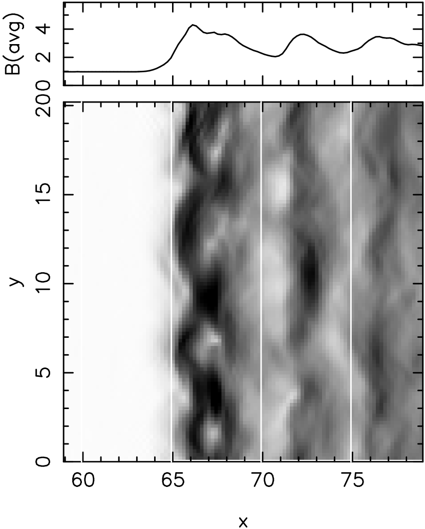
Figure 1: Gray scale map of magnetic field magnitude for Case A (see text) at time $T=20\Omega_{ci}^{-1}$ in the hybrid simulation. The white-black scale is $0.9-5.0$. The magnetic field averaged over the $y$ direction is shown in the upper panel. Only a small region of simulation around the shock is shown.

In this section we will illustrate the shock structure seen in hybrid simulations for a range of different shock and simulation parameters that will be used for the electron test particle simulations. The first example (Case A, Figure 1), and reference case, is for $\theta_{Bn}=87^{\circ}$, inflow velocity of $M_{i}=3.5$, and resultant shock Alfvén Mach number of $M_{A}=5.1$. In all examples here the ion and electron upstream plasma beta is $\beta_{i}=\beta_{e}=0.5$. Figure 1, upper panel, shows the magnetic field magnitude $B$ averaged over the $y$ direction. This average is rather stable over time, with only slight changes in form. The presence of the usual components of super-critical quasi-perpendicular shock structure is evident: foot, ramp, overshoot, and undershoot. Using the definition of the shock position given above, an instantaneous shock speed can be calculated. This shows some quasi-periodic variations on both short $\sim$0.1 $\Omega_{ci}^{-1}$ and longer $\sim$1.2 $\Omega_{ci}^{-1}$ time scales. This variation indicates small changes in the gradient and maximum value of the average $B$ profile; such behavior is also seen in one dimensional hybrid simulations.

Figure 1 (lower panel) shows a gray-scale map of the magnetic field magnitude in a small range of $x$ around the shock transition. The most obvious feature is that there is considerable structuring along the shock surface. Locally the field gradients are considerably larger than for the average profile. The shock surface has a rippled appearance, so that the local gradient normal changes in direction along the surface. The figure just shows the shock surface at one time, but the structure is highly dynamic on time scales of between 0.1 and 1.0 $\Omega_{ci}^{-1}$, with the pattern of ripples moving and changing in form. This can lead to rapid changes in the local angle between the upstream magnetic field and the gradient normal. Figure 1 shows the shock at a time when the rippling appears quasi-sinusoidal, but this feature is not constant; at other times the rippling is less coherent. The dynamic behavior of the shock structure has been analysed by Lowe & Burgess (2003) in terms of ripples propagating across the shock at approximately the Alfvén speed at the shock overshoot. Although we only show its magnitude, the perturbations in the shock layer occur strongly in all components of the magnetic field and the density (Winske & Quest, 1988).

All the cited work on two-dimensional hybrid shock simulations, and the above example, are for the case where the upstream magnetic field direction lies in the $x-y$ simulation plane. This allows the existence of perturbations with wave vectors parallel to the magnetic field direction, e.g., Alfvén ion cyclotron waves, which are known observationally to exist downstream of the supercritical quasi-perpendicular shock, and which therefore play an important role in ion thermalization at the shock transition (McKean et al., 1995). However, it is possible to place the upstream magnetic field direction in the $z-x$ plane, i.e., out of the simulation plane, so that the simulation cannot contain any perturbations propagating parallel to the field and transverse to the shock normal. This has the effect of suppressing Alfvén ion cyclotron and other predominantly parallel propagating waves.

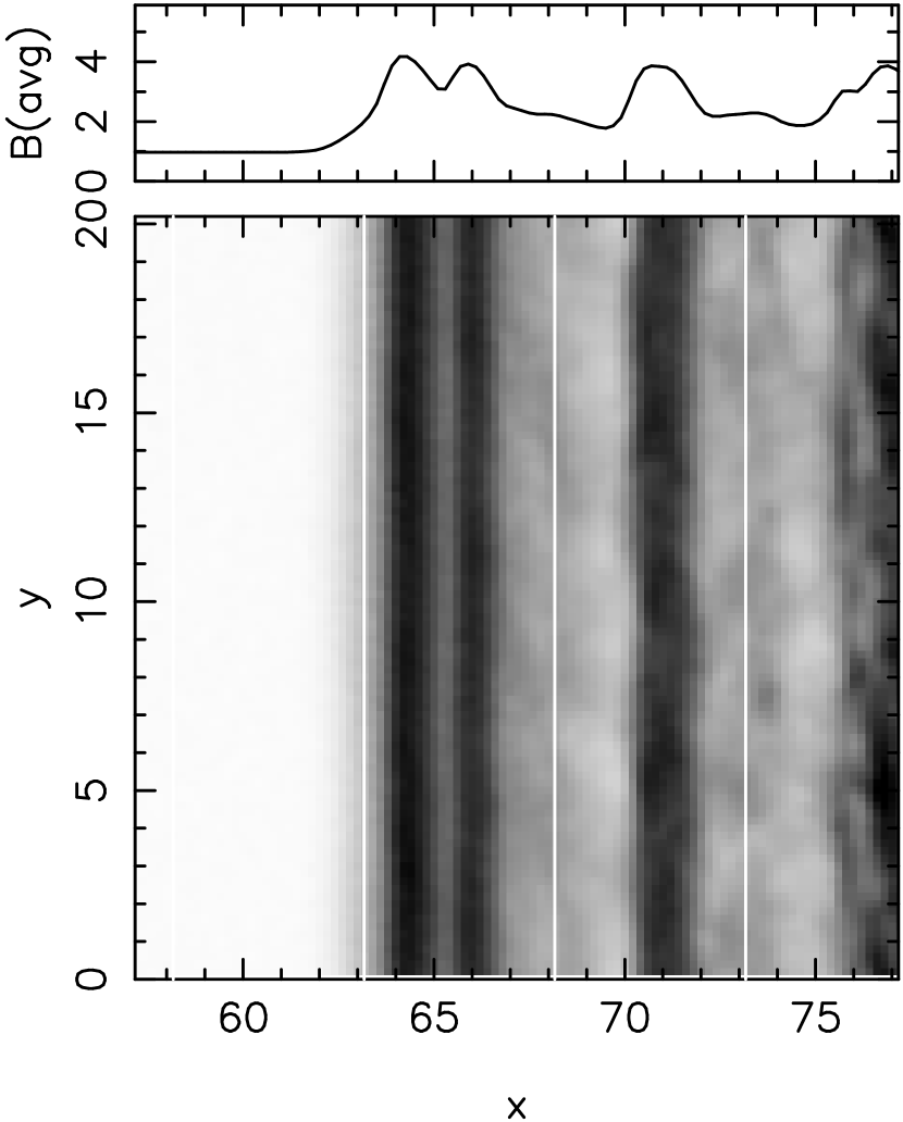
Figure 2: As Figure 1, but for Case B (see text).

Figure 2 illustrates this case (Case B), with $\mathbf{B}$ out of the simulation plane for the parameters $\theta_{Bn}=87^{\circ}$, inflow velocity of $M_{i}=3.2$, and resultant shock Alfvén Mach number of $M_{A}=5.1$. The inflow velocity has been adjusted so that the shock Mach number is the same as for Case A. This adjustment is necessary because the difference in the shock structure, which is clearly evident, leads to a different downstream thermalization, changing the propagation speed of the shock in the simulation frame. Although the appearance of the average profile is very similar to Case A, it is clear that putting the upstream field out of the simulation frame strongly suppresses any structuring of the shock transverse to the normal; the shock structure effectively becomes one dimensional. We should note that two-dimensional structuring of the shock can be found in simulations with $\mathbf{B}$ out of the simulation plane at higher Mach numbers. Although Case B is unrealistic, because perturbations propagating parallel to $\mathbf{B}$ are suppressed, we will be using it to demonstrate the role of dynamic shock structure in electron acceleration.

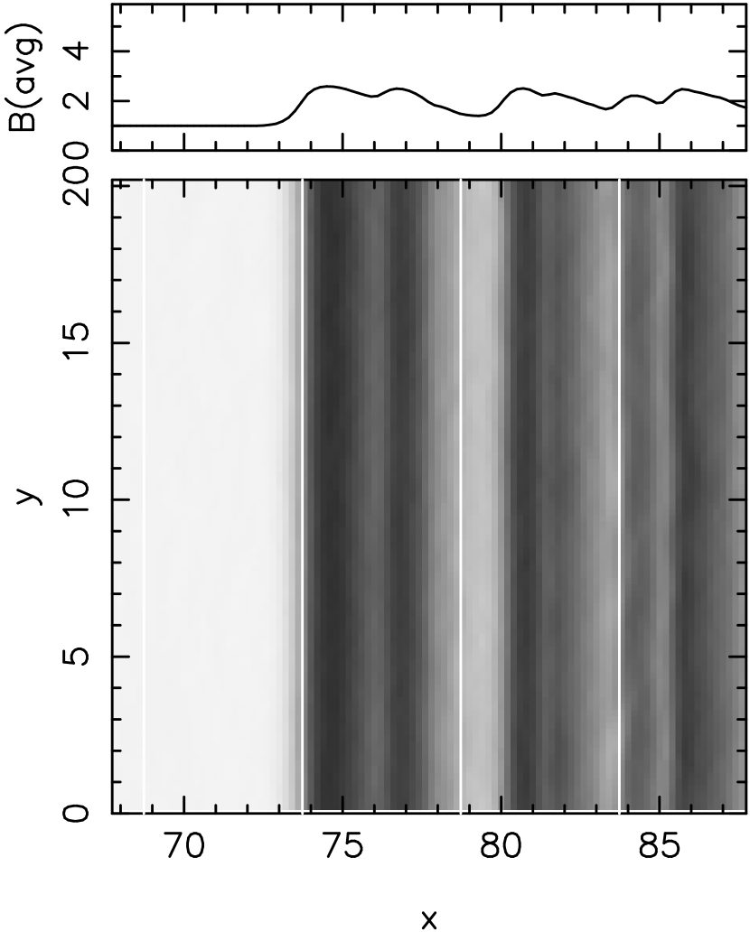
Figure 3: As Figure 1, but for Case C (see text). The white-black scale is $0.9-3.0$.

Lowe & Burgess (2003) reported that the rippled structuring of the shock is associated with the presence of an overshoot in the average magnetic field profile, i.e., the shock has to have a high enough Mach number to be supercritical, with the presence of reflected gyrating ions at the shock transition. We provide an example of this in Figure 3 (Case C), which shows the shock transition for a low Mach number shock with $\theta_{Bn}=87^{\circ}$, inflow velocity of $M_{i}=1.5$, and resultant shock Alfvén Mach number of $M_{A}=2.1$. The upstream magnetic field direction is in the simulation plane, as for Case A, but in comparison there is no appreciable overshoot in the magnetic field profile, and any rippling or variations of the shock surface is at a very low level. Again the shock structure is virtually one dimensional.

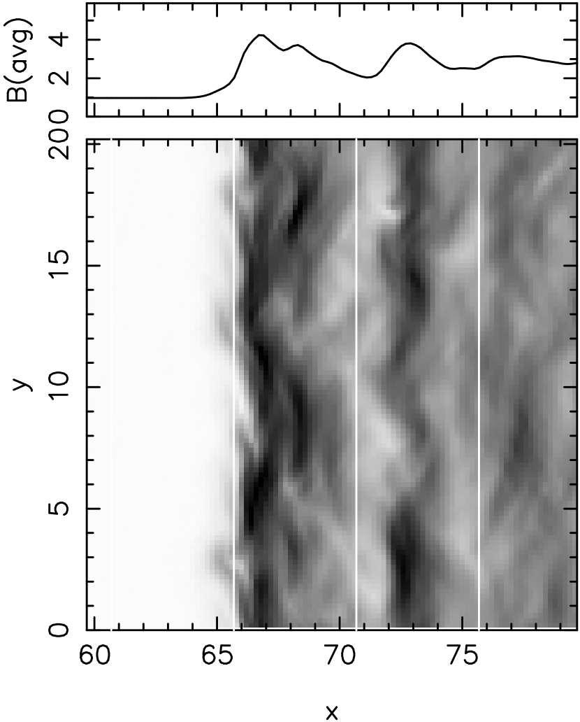
Figure 4: As Figure 1, but for Case D (see text).

So far a shock normal angle of $\theta_{Bn}=87^{\circ}$ has been used for all the examples. We will be showing the effect of $\theta_{Bn}$ on electron acceleration, and Figure 4 (Case D) shows the shock structure for the lower value of $\theta_{Bn}=80^{\circ}$, but with other parameters the same as Case A. Comparing with Case A, the profile of the average magnetic field is very similar, and the two dimensional structuring is also basically similar. There are some differences of appearance; the shock transition for the lower $\theta_{Bn}$ case has a slightly more fractured appearance, with the more evident presence of precursor waves, presumably associated with oblique whistlers. Again, as for Case A, the shock transition structuring is highly dynamic in time and space.

3.2 Electron Energy Spectra

The structure and variability within the shock transition modeled by the two dimensional hybrid simulation has a major effect on the spectra of shock accelerated electrons in the energy range up to about 10 keV. This is demonstrated in Figure 5 which shows the upstream energy spectra for an initial energy $E_{i}=1$ keV for Case A (reference simulation), Case B ($\mathbf{B}$ out of simulation plane) and Case C ($\mathbf{B}$ in simulation plane, but low $M_{A}$). Case A shows considerable structuring and variability, whereas Cases B and C show little or no structuring of the shock front. Three important features are evident in the spectrum for Case A: The maximum energy achieved is much greater than for the other cases, by a factor of almost 10. There is a region, roughly $2-6$ keV, where the variation of the differential energy flux is almost flat. Finally, above 6 keV the spectrum falls off with a power law dependence with a slope of approximately $-4.6$.

The cases without a rippled shock structure have much smaller maximum energies, and a sharp cut-off with increasing energy. The peak energies for these cases are in line with the prediction of adiabatic reflection theory, as is the sharp upper limit. The low Mach number spectrum (Case C) shows a smaller peak energy, again consistent with adiabatic reflection theory. For case B, which has the same Mach number as Case A, the flux at low energies is greater than for Case A, but then Case A displays considerably higher (by many orders of magnitude) fluxes at higher energy.

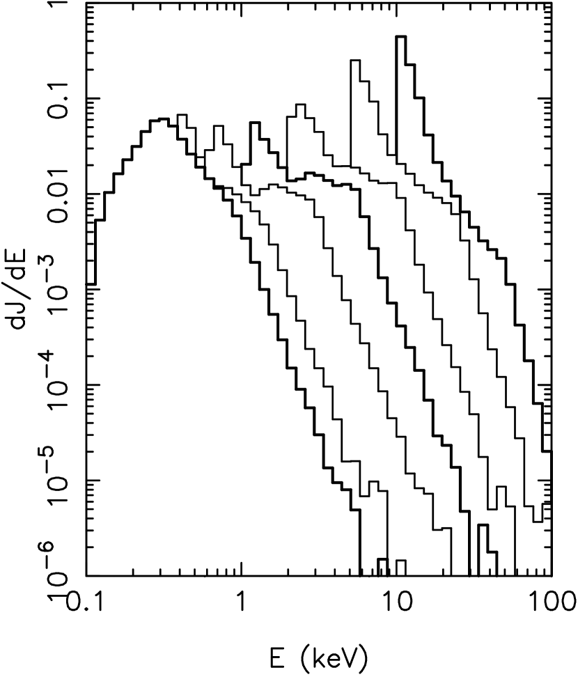
Figure 6: Energy spectra for Case A for electron injection energies of 100 eV, 200 eV, 500 eV, 1 keV, 2 keV, 5 keV, and 10 keV.

Figure 6 shows the spectra for a range of injection energies $E_{i}$ from 100 eV to 10 keV for case A, which has dynamic structuring across the shock surface and along the magnetic field lines. All spectra show a transition to a power law fall off above a certain energy. The spectrum for $E_{i}=100$ eV shows, after its peak value, a fall off with a change of slope around 1 keV. For $E_{i}>100$ eV all spectra have a peak in the range up to about $2E_{i}$, typical of a single reflection interaction. Recall that the algorithm for removal of particles which are headed away from the shock introduces some error at the lower edge of the spectra.

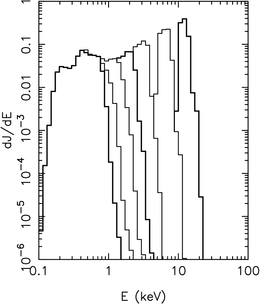
Figure 7: As for Figure 6, but for the shock Case B which does not show a structured shock front.

The most prominent feature is that part of the spectrum which is almost flat for injection energies in the range 500 eV to 2 keV. This feature begins to be evident around $E_{i}=200$ eV, for which there is a narrow peak, a small region of shallower slope, and then a steeper power law fall off. Beyond $E_{i}=2$ keV, the spectrum does not have a flat plateau region, but instead a region of shallower slope, and the slope steepens with increasing injection energy. Thus, by $E_{i}=10$ keV the spectrum shows a peak up to 20 keV, then a fall off which changes slopes and steepens at around 50 keV. In contrast to the results for Case A, Figure 7 shows the spectra for a similar range of injection energies, but for Case B, where the structuring along the shock front and magnetic field direction has been suppressed by putting the upstream magnetic field direction out of the simulation plane. In this case all spectra show an extremely rapid fall off with increasing energy, consistent with reflection from a one dimensional shock structure.

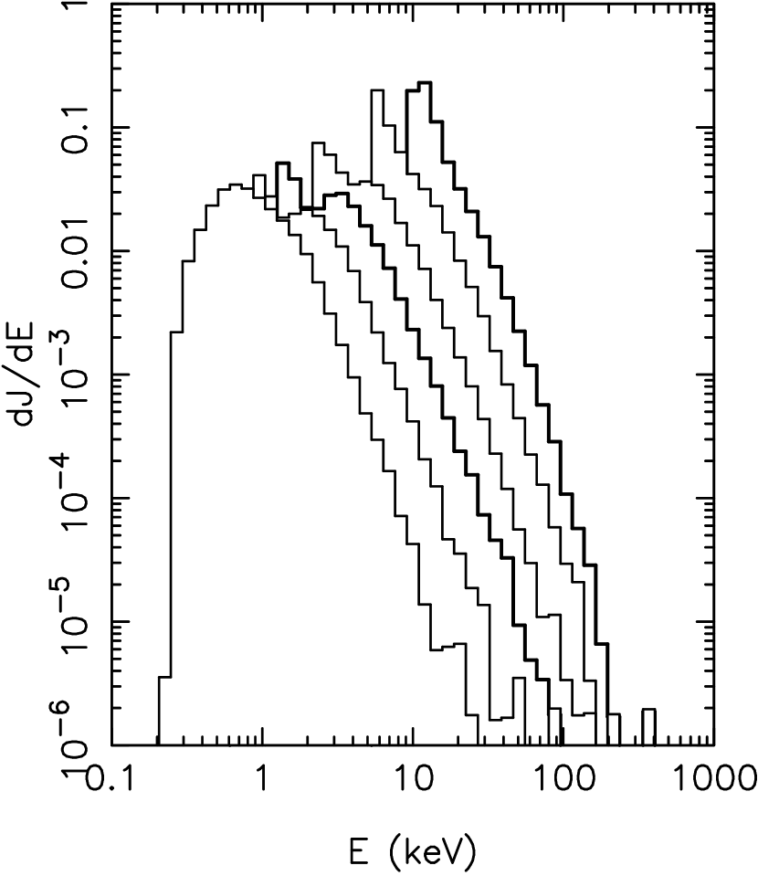
Figure 8: Energy spectra for a shock similar to Case A, but with $\theta_{Bn}=88^{\circ}$, for electron injection energies of 200 eV, 500 eV, 1 keV, 2 keV, 5 keV, and 10 keV

The shock normal angle $\theta_{Bn}$ is a crucial parameter in adiabatic reflection theory for electron acceleration. Figure 8 shows the spectra for $E_{i}$ from 200 eV to 10 keV for a simulation with the same parameters as Case A, but with $\theta_{Bn}=88^{\circ}$. The overall behavior is very similar to the results for $\theta_{Bn}=87^{\circ}$ (Figure 6): a plateau region (now with a definite secondary peak) is present for an intermediate range of injection energy, and a power law decrease at higher energies. The slope is independent of injection energy. However, for $E_{i}=5$ keV and 10 keV there is a single power law decrease, over 5 orders of magnitude, from the injection energy up to about 100 keV. There is some indication that the fall off is more rapid above 100 keV.

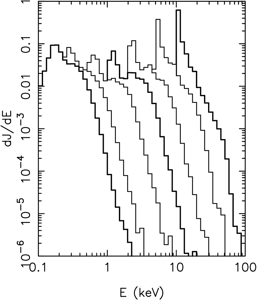
Figure 9: As for Figure 6 for a shock similar to Case A, but with $\theta_{Bn}=85^{\circ}$

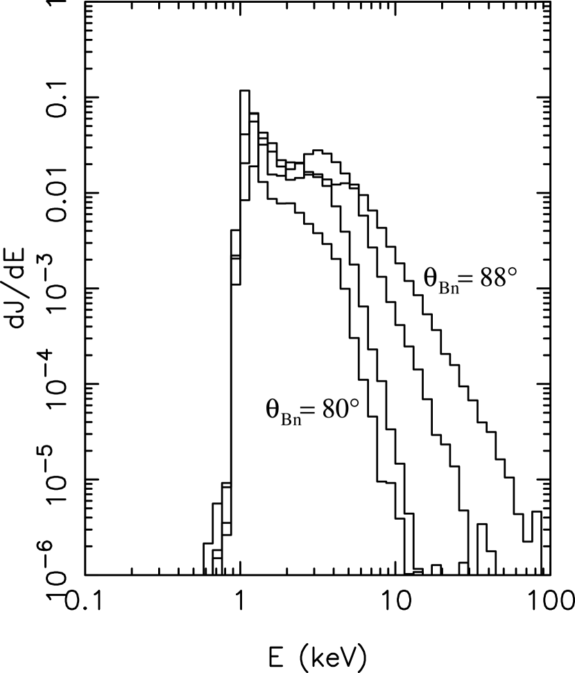
Figure 10: Energy spectra for a fixed injection energy of 1 keV for a set of shocks similar to Case A, but with $\theta_{Bn}=80^{\circ}$, $85^{\circ}$, $87^{\circ}$, and $88^{\circ}$.

Figure 9 shows the spectra for $E_{i}$ from 100 eV to 10 keV for a similar simulation with a lower value of $\theta_{Bn}=85^{\circ}$. Once again the spectra show broadly the same features as for $\theta_{Bn}=87^{\circ}$, although the maximum energies achieved are lower. The effects of $\theta_{Bn}$ on the fall off slope and flux levels are illustrated in Figure 10, which shows the energy spectra for $E_{i}=1$ keV for $\theta_{Bn}=80^{\circ}$, 85^∘, 87^∘, and 88^∘. The effect of increasing $\theta_{Bn}$ is to increase the maximum energy at a given flux level, to emphasize the appearance of the plateau/secondary peak region of the spectrum, and to decrease the slope of power law decrease. The power slope varies from -3.1 at $\theta_{Bn}=88^{\circ}$ to -7.0 at $\theta_{Bn}=80^{\circ}$. Another key feature is that the flux levels in the intermediate portion of the spectrum are all approximately equal in the range $\theta_{Bn}=85^{\circ}-88^{\circ}$ (and presumably above). Even at $\theta_{Bn}=80^{\circ}$, the flux levels are only down by a factor $0.1-0.5$. This indicates that the acceleration mechanism in the intermediate range operates over a reasonably wide range of $\theta_{Bn}$, at least when compared to adiabatic reflection theory, which is often characterized as most effective above $\theta_{Bn}=88^{\circ}$.

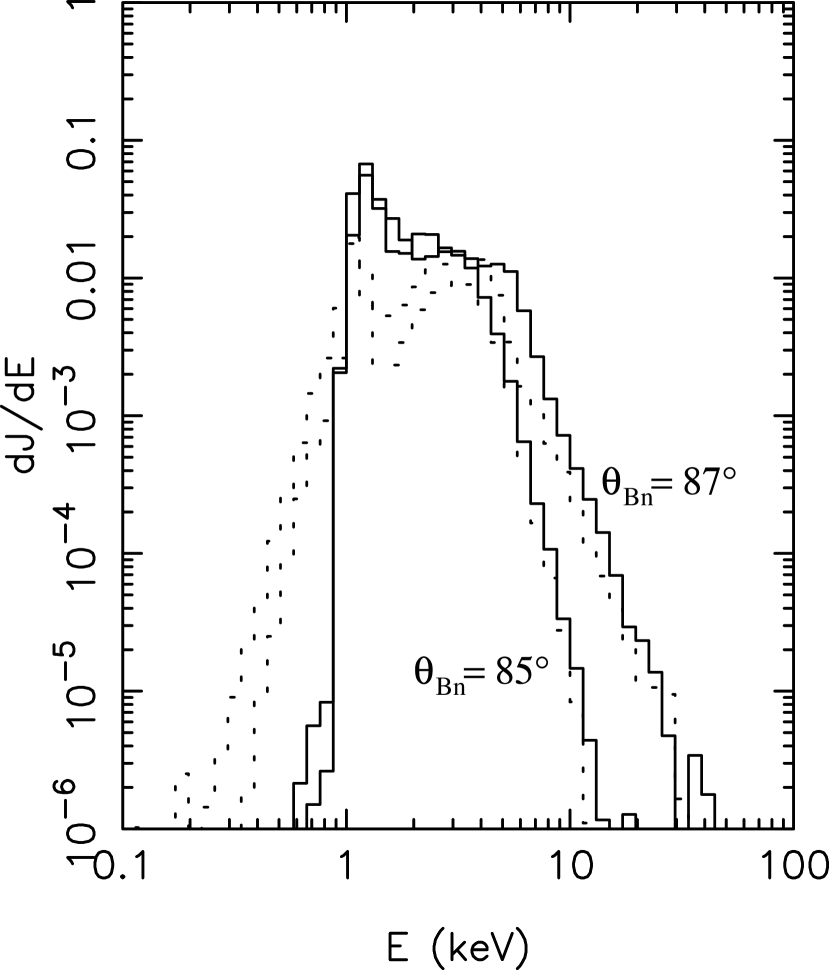
Figure 11: Upstream (solid) and downstream (dotted) energy spectra for fixed injection energy of 1 keV for two shocks: Case A with $\theta_{Bn}=87^{\circ}$, and a similar shock with $\theta_{Bn}=85^{\circ}$.

Finally, we have so far concentrated on the results for electrons collected upstream, since the reflected population is the most studied case at the Earth’s bow shock in terms of observations and implications for waves in the foreshock. Figure 11 compares the upstream and downstream spectra for an injection energy of 1 keV for $\theta_{Bn}=88^{\circ}$ and $\theta_{Bn}=85^{\circ}$. Especially striking is the fact that the upstream and downstream spectra for the region of power law fall off, beyond the the plateau region, are almost exactly the same in terms of level and slope. This is a very general property for all the cases we have studied where the upstream magnetic field lies in the simulation plane, i.e., where the shock has dynamic rippled structuring. The greatest difference between the upstream and downstream spectra is in the range $1-3$ keV; there are greater differences as $\theta_{Bn}$ decreases. For example, at $\theta_{Bn}=85^{\circ}$, there is no plateau region in the downstream spectrum, whereas the upstream spectrum shows a plateau region at a high flux level. The similarity of the upstream and downstream spectra can be shown to be directly linked to the presence of dynamic shock structure. Figure 12 shows the comparison between the upstream and downstream spectra (for $E_{i}=1$ and $10$ keV) for a shock simulation where the structuring along the shock surface is suppressed (Case B). There are major differences between the level and form of the upstream and downstream spectra. The downstream spectra shows hardly any energization, with the upstream flux at a very much higher level at all energies above the injection energy. As discussed above, the upstream spectra themselves have a steep fall off with energy.

4 Summary

The work presented here extends earlier work studying fast Fermi shock acceleration of electrons using self-consistently simulated shock fields. A two dimensional hybrid shock simulation has been used, which shows dynamic rippled structure across the shock surface and along the magnetic field direction. This structuring produces a radically different behavior compared with a one dimensional shock. Our results indicate that suprathermal electrons can be scattered within the shock transition even without strong electron scale fluctuations. For a shock with $M_{A}=5$ and using test particle electrons with injection energies in the range $100-10$ keV, we find energy spectra of differential flux to have a “plateau” region (either flat or shallow sloped) in an intermediate energy range up to $2-5$ times the injection energy, with a larger range at lower energies. Above the plateau region of the spectrum, there is an inverse power law form, the slope of which increases as $\theta_{Bn}$ decreases. Above a certain energy the downstream and upstream spectra are effectively the same. The accelerated fluxes are present over an extended range of $\theta_{Bn}$, not just immediately close to $90^{\circ}$, as found for adiabatic reflection theory. All these principle results are in general agreement with observations. As such, these results have implications for models of electron acceleration at planetary bow shocks, interplanetary shocks (and similar other astrophysical shocks) and also for models of nonthermal radio-emission which depend on accelerated electrons. More detailed comparisons between the simulations and observations will use an initial electron distribution, rather than the mono-energetic release used here.

The similarity of the downstream and upstream spectra above some energy indicates that the electron motion within the shock transition is strongly affected by a scattering process, which is not surprising given the level of fluctuation at the shock surface. At lower energies, however, there is a clear signature of the adiabatic reflection process. This suggests that both processes play a role: an initial energization is produced by magnetic mirroring, but scattering on magnetic fluctuations keeps particles within the shock transition, and allows stochastic acceleration. Particles with suitable energy and pitch angle at the edges of the shock transition region can then escape either upstream or downstream. A scenario with strong scattering in the shock transition will produce two effects: an increase in accelerated electron flux at the shock itself, i.e., a “shock spike event” as observed at the Earth’s bow shock (Gosling et al., 1989) and interplanetary shocks (Tsurutani & Lin, 1985); and near isotropic downstream distributions with the upstream “reflected” population emerging from the downstream distribution in the shock ramp, as observed at the bow shock (Gosling et al., 1989).

The use of a hybrid simulation to provide the electric and magnetic fields means that electron scale (in the simulation frame) fluctuations are not included. Consequently, our results may not be appropriate for shocks which have strong electron heating and therefore strong electron scale turbulence. This is not generally the case for planetary and interplanetary shocks. The validity of neglecting such electron scale fluctuations can only be validated by (at least two dimensional) full particle simulations with careful use of appropriate simulation parameters (see discussion in Section 1). However, even if, for some given shock, there is a non-negligible effect from electron scale turbulence, then the process described in this paper will still operate, provided that there is dynamic rippled structuring of the shock front. In this case, the relative importance of the two processes will have to be evaluated.

Our key results, such as inverse power law energy spectra and extended range of effective $\theta_{Bn}$, are due to the presence of shock surface fluctuations, which have, in turn, been shown to be present only if the shock Mach number is high enough. This provides a key observational test, since interplanetary shocks cover a wide range of Mach number. Also, Type II solar radio bursts show considerable variability, and this may be due to the associated interplanetary shock changing Mach number as it propagates through an inhomogeneous solar wind (c.f., Knock et al., 2003). Our results show that a low Mach number shock should exhibit the features of scatter free adiabatic reflection theory: upstream maximum energization close to $\theta_{Bn}=90^{\circ}$ with a limited energy range, and anisotropic downstream distributions with little energization. However, this picture maybe modified if the shock is propagating through turbulence. It is possible that fluctuations of the appropriate scale lengths are amplified at the shock, thereby producing scattering in the same way as the surface fluctuations at the high Mach number shocks simulated here.

We have presented results for mono-energetic injection, thereby demonstrating the overall operation and behavior of the process and the range of parameters for which it is effective. Future work will present the evolution of the energetic electron distribution function across the shock, and the spectra and anisotropies for model input distribution functions, thereby facilitating comparisons with observations

Figure 5: Upstream differential flux energy spectra for an injection energy of 1 keV for: Case A (thick line), Case B (thin line), and Case C (dotted line). Case A has a shock surface with dynamic rippled structure, while the others have a quasi-one dimensional structure.

Figure 12: Upstream (solid) and downstream (dotted) energy spectra for Case B (without shock surface structuring) for injection energies of 1 keV and 10 keV.

References

- Anderson et al. (1979) Anderson, K. A., Lin, R. P., Martel, F., Lin, C. S., Parks, G. K., & Rème, H. 1979, Geophys. Res. Lett., 6, 401
- Bessho & Ohsawa (2002) Bessho, N., & Ohsawa, Y. 2002, Physics of Plasmas, 9, 979
- Burgess (1995) Burgess, D. 1995, in Introduction to Space Physics, M. G. Kivelson and C. T. Russell (eds) (Cambridge: Cambridge University Press), 129–163
- Cairns (1987) Cairns, I. H. 1987, J. Geophys. Res., 92, 2315
- Cargill & Papadopoulos (1988) Cargill, P. J., & Papadopoulos, K. 1988, ApJ, 329, L29
- Fitzenreiter et al. (1990) Fitzenreiter, R. J., Scudder, J. D., & Klimas, A. J. 1990, J. Geophys. Res., 95, 4155
- Gosling et al. (1989) Gosling, J. T., Thomsen, M. F., Bame, S. J., & Russell, C. T. 1989, J. Geophys. Res., 94, 10011
- Holman & Pesses (1983) Holman, G. D., & Pesses, M. E. 1983, ApJ, 267, 837
- Knock et al. (2003) Knock, S. A., Cairns, I. H., Robinson, P. A., & Kuncic, Z. 2003, J. Geophys. Res., 108, 6
- Krauss-Varban (1994) Krauss-Varban, D. 1994, J. Geophys. Res., 99, 2537
- Krauss-Varban & Burgess (1991) Krauss-Varban, D., & Burgess, D. 1991, J. Geophys. Res., 96, 143
- Krauss-Varban et al. (1989) Krauss-Varban, D., Burgess, D., & Wu, C. S. 1989, J. Geophys. Res., 94, 15089
- Krauss-Varban & Wu (1989) Krauss-Varban, D., & Wu, C. S. 1989, J. Geophys. Res., 94, 15367
- Kuncic et al. (2004) Kuncic, Z., Cairns, I. H., & Knock, S. A. 2004, J. Geophys. Res., 109, A02108
- Lembège & Savoini (2002) Lembège, B., & Savoini, P. 2002, Journal of Geophysical Research (Space Physics), 107
- Leroy & Mangeney (1984) Leroy, M. M., & Mangeney, A. 1984, Annales Geophys., 2, 449
- Lowe & Burgess (2003) Lowe, R. E., & Burgess, D. 2003, Ann. Geophys., 21, 671
- Matthews (1994) Matthews, A. P. 1994, J. Comp. Phys., 112, 102
- McKean et al. (1995) McKean, M. E., Omidi, N., & Krauss-Varban, D. 1995, J. Geophys. Res., 100, 3427
- Savoini & Lembège (2001) Savoini, P., & Lembège, B. 2001, J. Geophys. Res., 106, 12975
- Schmitz et al. (2002) Schmitz, H., Chapman, S. C., & Dendy, R. O. 2002, ApJ, 579, 327
- Scholer et al. (2003) Scholer, M., Shinohara, I., & Matsukiyo, S. 2003, J. Geophys. Res., 108, 4
- Simnett et al. (2005) Simnett, G. M., Sakai, J.-I., & Forsyth, R. J. 2005, A&A, 440, 759
- Thomsen (1968) Thomsen, W. E. 1968, Comput. J., 10, 417
- Tsurutani & Lin (1985) Tsurutani, B. T., & Lin, R. P. 1985, J. Geophys. Res., 90, 1
- Vandas (1995) Vandas, M. 1995, J. Geophys. Res., 100, 23499
- Vandas (2001) —. 2001, J. Geophys. Res., 106, 1859
- Vandas & Karlický (2000) Vandas, M., & Karlický, M. 2000, Sol. Phys., 197, 85
- Winske & Quest (1988) Winske, D., & Quest, K. B. 1988, J. Geophys. Res., 93, 9681
- Wu (1984) Wu, C. S. 1984, J. Geophys. Res., 89, 8857