Data Analysis on the Extra-solar Planets Using Robust Clustering

Abstract

We use both the conventional and more recently developed methods of cluster analysis to study the data of extra-solar planets. Using the data set with planetary mass $M$, orbital period $P$, and orbital eccentricity $e$, we investigate the possible clustering in the ${\rm ln}M$, ${\rm ln}P$, ${\rm ln}P-{\rm ln}M$, $e$, and ${\rm ln}P-e$ spaces. There are two main implications: (1) mass distribution is continuous and (2) orbital population could be classified into three clusters, which correspond to the exoplanets in the regimes of tidal, on-going tidal and disc interaction, respectively.

Key words: data analysis, cluster analysis, planetary systems, stellar dynamics.

1 Introduction

Astronomers’ observational efforts have led to the detection of more than 160 extra-solar planets (exoplanets). These discoveries open a new window to astronomy, which could eventually lead to answers to the fundamental questions about the formation of planetary systems, including our Solar System. In fact, some of the work has already been done to address the important questions about planetary evolution. For example, Zakamska & Tremaine (2004) tried to explain the high eccentricities of exoplanets by possible stellar encounters. Ji et al. (2002, 2003) have studied the orbital evolutions of a few known resonant planetary systems. Veras & Armitage (2004) proposed the possible mechanisms to make exoplanets migrate outward. Jiang & Ip (2001) investigated the origin of orbital elements of the planetary system of upsilon Andromedae. Yeh & Jiang (2001) studied the orbital migration of scattered planets. Jiang & Yeh (2004a, 2004b) did some analysis on the orbital evolution of systems with planet-disc interaction.

While the number of detected planets keep increasing, it is important to study the distributions of their masses, periods, and other orbital elements. The details of these distributions could have crucial implications for the formation and evolution of planetary systems. It is quite common that we use a simple function, say, a power law, to model the distribution of a quantity in our system (Tabachnik & Tremaine 2002). It also happens that, after a further study, we find that a single power-law is not good enough and we make the change to a double-power-law. This process will eventually help us to understand the properties of the system.

On the other hand, cluster analysis, which is a data analysis tool to find clusters of a data set with the most similarity in the same cluster and the most dissimilarity between different clusters, might also help us to distinguish a double-power-law from a single power-law for a particular study from another point of view. When we find that there is only one group (or a huge number of groups) through cluster analysis, it is likely that a simple function (say, a single power-law) could be a good approximation. When there are two or more groups in cluster analysis, we might need a combination of several functions (say, double-power-law) to model the data set. In this way, we can be more confident of the results derived from the usual conventional process. Another advantage of cluster analysis is that it can also be used to study the distributions of multi-variables easily.

Clustering is a powerful exploratory approach to find groups in data and to reveal the structure information of a given data set. It is a data driven procedure to classify a datum in one of a few classes by looking at proximity and homogeneity in feature space. Conventional approaches to clustering can be grouped into two categories namely partitional and hierarchical. The $k$-means (see MacQueen 1967, Hartigan 1975) algorithm is a popular example of partitional clustering whereby the data is partitioned into $k$ classes with the value of $k$ known a priori. Single linkage algorithm (Gower and Ross 1969, Hartigan 1967) is an example of hierarchical agglomerative clustering where for $n$ data a hierarchy of clusters ranging from $n$ to $1$ is formed.

The single linkage algorithm was used in asteroid studies (Zappala et al. 1995) and in many meteoroid stream searches (Baggaley & Galligan 1997, Galligan 2003a, Galligan 2003b). Zappala et al. (1995) identified the dynamical families from a sample of 12,487 asteroids. They divided the main asteroid belt into three different zones (the inner, intermediate, and outer zone) and study the hierarchical structures of the orbital families. Baggaley & Galligan (1997) first used the single linkage algorithm to work on meteoroid stream data from the Advanced Meteoroid Orbit Radar (AMOR). They probed the structure of the orbital distributions and determined the extent of dynamical families or clusters in the population. Moreover, in order to determine a reasonable cut-off level, they also introduced the combination of the single-linkage method with a randomization technique. Galligan (2003a, 2003b) further studied more recent AMOR data by these methods.

From the previous work, we can see that the cut-off level in the conventional single linkage method would influence the results of clustering and therefore the number of clusters. In Section 2, we first briefly review the single linkage algorithm. We then review the much more advanced method called the similarity-based clustering method (SCM) proposed by Yang & Wu (2004) in Section 3. Some numerical examples and comparisons between the single linkage algorithm and the SCM are made in Section 4. Section 5 starts our applications of the single linkage algorithm and the SCM on the data of exoplanets. The implications of these results on the formation and evolution of planetary systems will also be given in Section 5. Section 6 concludes the paper.

2 The Single Linkage Algorithm

The clustering process begins with measures of the distance of the objects from one another. Several measures are available, but we shall use simple Euclidean distance in most cases. Usually, the distances can be summarized in a symmetric $n\times n$ matrix $D=(d_{ij})$, where $d_{ij}$ is the Euclidean distance between objects $i$ and $j$. We illustrate the single linkage algorithm with the artificial distance matrix given by Johnson & Wichern (1988)

$$D=\left[\begin{array}[]{ccccc}0&&&&\\ 9&0&&&\\ 3&7&0&&\\ 6&5&9&0&\\ 11&10&2&8&0\end{array}\right].$$

The minimum distance occurs between objects $3$ and $5$, so the first cluster, labelled as (35), will consist of those objects. The second matrix of distances is formed by deleting the rows and columns of $D$ corresponding to objects $3$ and $5$, and adding a row and column with the distances of the remaining objects from the cluster (35). Those distances are found from the rule

$$d_{(35),1}=\min\{d_{31},d_{51}\}=\min\{3,11\}=3$$

$$d_{(35),2}=\min\{d_{32},d_{52}\}=\min\{7,10\}=7$$

$$d_{(35),4}=\min\{d_{34},d_{54}\}=\min\{9,8\}=8.$$

The minimum distance in the second matrix is $d_{(35),1}=3$ and we merge cluster (1) with cluster (35) to get the next cluster, (135). Next, we form a third distance matrix: for it we note that

$$d_{(135),2}=\min\{d_{(35),2},d_{12}\}=\min\{7,9\}=7$$

$$d_{(135),4}=\min\{d_{(35),4},d_{14}\}=\min\{8,6\}=6.$$

The minimum distance in the third matrix is $d_{42}=5$ and we merge objects 4 and 2 to get the cluster (24). At this time we have two distinct clusters, (135) and (24). Their minimum distance is

$$d_{(135),(24)}=\min\{d_{(135),2},d_{(135),4}\}=\min\{7,6\}=6.$$

Therefore, clusters (135) and (24) are merged to form a single cluster of all five objects, (12345), when the minimum distance reaches 6.

The clusters are illustrated in the dendrogram of Fig. 1. The dendrogram is formed by plotting the minimum distances for each cluster in a tree configuration leading to the single cluster of all $5$ objects. The objects should be ordered so that the branches of the dendrogram stand alone without crossing. The dendrogram clearly suggests that the sample may contain two sets of objects: $(135)$ and $(24)$.

In general, single linkage algorithm, which combines the original $n$ single-object clusters hierarchically into one cluster of $n$ objects, cab be summarized as:

Single Linkage Algorithm

• Start with $n$ single-object clusters. The distances are described by the initial distance matrix $D=(d_{ij})$.

• Search for the nearest pair of clusters from the distance matrix. When there are more than one candidate pairs, randomly pick one of them. Let the distance between this pair of clusters, $U$ and $V$, be $d_{UV}$, where

  $$d_{UV}=\min_{u\in U,v\in V}\{d_{uv}\}.$$

• Merge clusters $U$ and $V$. Label the newly formed cluster as $(UV)$. Form a new distance matrix by (i) deleting the rows and columns corresponding to clusters $U$ and $V$ and (ii) adding a row and column giving the distances between cluster $(UV)$ and the remaining clusters. The distances between cluster $(UV)$ and any other cluster $W$ are computed by

  $$d_{(UV)W}=\min\{d_{UW},d_{VW}\},$$

  where $d_{UW}$ and $d_{VW}$ are the distances between clusters $U$ and $W$ and clusters $V$ and $W$, as defined in S2.

• Repeat S2 and S3. All objects will be in a single cluster at the termination of the algorithm. Record the identity of clusters that are merged and the levels at which the mergers take place.

The above clustering results of single linkage algorithm can be graphically displayed in the form of a dendrogram, which shows the clustering structure at various levels of the hierarchy. The branches in the tree represent clusters. The branches come together (merge) at nodes whose positions along a distance axis indicate the level at which the fusions occur. Therefore, the vertical axis indicates the distance and the horizontal axis simply shows the data identity numbers.

Please note that the dendrogram plotted in Baggaley & Galligan (1997) is slightly different from what we just described here. In their plot, the meaning of the horizontal axis is different from ours. Due to the huge number of orbits, their horizontal axis shows the scale of number of clustering members. The meaning of their vertical axis is the same as ours.

3 The Similarity-Based Clustering Method

Let the data set be $X=\{x_{1},\cdots,x_{n}\}$ where $x_{j}$ is a feature vector in the $s$-dimensional Euclidean space $\Re^{s}$ and $c$ is the specified number of clusters. Yang and Wu (2004) considered maximizing the objective function $J(z)$ with

$$J(z)=\sum_{i=1}^{c}\sum_{j=1}^{n}\Big{(}\exp-\frac{||x_{j}-z_{i}||^{2}}{\beta}\Big{)}^{\gamma},$$ (1)

where $\exp(-\frac{||x_{j}-z_{i}||^{2}}{\beta})$ is the similarity measure between $x_{j}$ and the $i$th cluster center $z_{i}$, $||x_{j}-z_{i}||$ is the Euclidean norm, $\gamma>0$ and

$$\beta=\frac{\sum_{j=1}^{n}||x_{j}-\bar{x}||^{2}}{n},\,\,\mbox{where}\,\,\bar{x}=\frac{1}{n}\sum_{j=1}^{n}x_{j}.$$

Since the clustering result is influenced by $\gamma$, Yang and Wu (2004) proposed correlation comparison algorithm (CCA) to select $\gamma$. According to the fact that the parameter $\gamma$ controls the location of the peaks of $J(z)$, they considered the total similarity function $\tilde{J}(x_{k})_{\gamma_{m}}$ for each data point $x_{k}$ with

$$\tilde{J}(x_{k})_{\gamma_{m}}=\sum_{j=1}^{n}\Big{(}\exp-\frac{||x_{j}-x_{k}||^{2}}{\beta}\Big{)}^{\gamma_{m}},~{}k=1,\cdots,n,$$

where $\gamma_{m}=5m$, $m=1,2,3,\cdots$. The correlation between the values of $\tilde{J}(x_{k})_{\gamma_{m}}$ and $\tilde{J}(x_{k})_{\gamma_{m+1}}$ are calculated. That is, CCA is based on a correlation comparison procedure with “$\gamma_{1}=5,\gamma_{2}=10$”, “$\gamma_{2}=10,\gamma_{3}=15$”, “$\gamma_{3}=15,\gamma_{4}=20$”, $\cdots$ etc. The CCA then is summarized as follows:

Correlation Comparison Algorithm (CCA)

• Set $m=1$ and give a threshold $\epsilon_{1}$.

• Calculate the correlation of the values of $\tilde{J}(x_{k})_{\gamma_{m}}$ and $\tilde{J}(x_{k})_{\gamma_{m+1}}$.

• If the correlation is greater than or equal to the threshold $\epsilon_{1}$

• THEN choose $\gamma_{m}$ to be the estimate of $\gamma$;

• ELSE $m=m+1$ and GOTO S2.

Since Yang and Wu (2004) suggested a threshold around $0.97\sim 0.999$, we choose 0.99 for the threshold in this paper. After the parameter $\gamma$ is estimated using CCA, the next step is to find a $z_{i}$ that maximizes the SCM objective function $J(z)$. Differentiating $J(z)$ with respect to all $z_{i}$, we obtain

$$\frac{dJ_{(}z)}{dz_{i}}=\sum_{j=1}^{n}2\frac{\gamma}{\beta}(x_{j}-z_{i})\Big{(}\exp-\frac{||x_{j}-z_{i}||^{2}}{\beta}\Big{)}^{\gamma}$$ (2)

and set (2) to zero. The necessary condition that maximizes $J_{(}z)$ is

$$z_{i}=\frac{\sum_{j=1}^{n}x_{j}\Big{(}\exp(-\frac{||x_{j}-z_{i}||^{2}}{\beta})\Big{)}^{\gamma}}{\sum_{j=1}^{n}\Big{(}\exp(-\frac{||x_{j}-z_{i}||^{2}}{\beta})\Big{)}^{\gamma}}.$$ (3)

This necessary condition can be decomposed into two conditions. First, we take the similarity relation $S(x_{j},z_{i})$ with

$$S_{ij}=S(x_{j},z_{i})=\exp\Big{(}-\frac{||x_{j}-z_{i}||^{2}}{\beta}\Big{)}$$ (4)

and then the necessary condition (3) becomes

$$z_{i}=\frac{\sum_{j=1}^{n}S_{ij}^{\gamma}x_{j}}{\sum_{j=1}^{n}S_{ij}^{\gamma}}.$$ (5)

This forms the similarity clustering algorithm (SCA). Thus, after the CCA is implemented to get an estimate $\gamma$, the SCA will be used to find the peaks of the SCM objective function is then summarized as follows:

Similarity Clustering Algorithm (SCA)

• Initialize $z_{i}^{(0)},i=1,\cdots,c$ and give $\epsilon$;

• Set iteration counter $\ell=0$;

• Estimate $S_{ij}^{(\ell+1)}$ by Eq.(4);

• Estimate $z_{i}^{(\ell+1)}$ by Eq.(5);

• Increment $\ell$; Until $\displaystyle\max_{i}||z_{i}^{(\ell+1)}-z_{i}^{(\ell)}||<\epsilon$.

When one processes SCA, all the cluster centers, $z_{i}$, will change positions for each iteration. If the data set has only one peak on the SCM objective function, all the centers will gradually centralize to that unique peak. In this case, we will claim there is only one cluster for this data set. When the data set has more than one peak on the SCM objective function, we can randomly give more initial cluster centers to process SCA and these centers will then centralize to the peaks of the SCM objective function. The problem here is what kind of the initialization can guarantee that all peaks (clusters) will be found simultaneously. To solve this problem, Yang and Wu (2004) suggested to set all data points to be the initial centers (i.e., $z^{(0)}=(z_{1}^{(0)},\cdots,z_{n}^{(0)})=(x_{1},\cdots,x_{n}))$. They successfully showed that all peaks (clusters) will be found for this initialization.

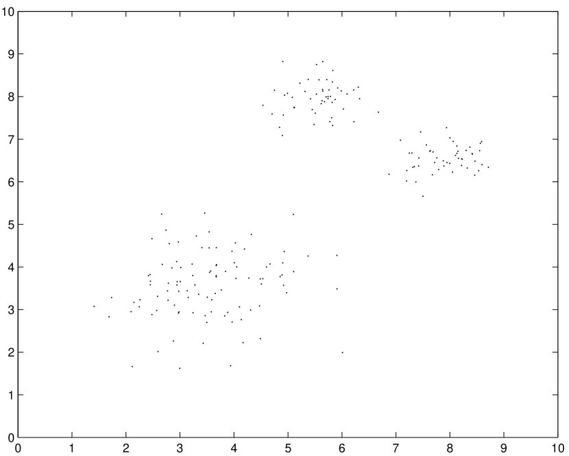
Figure 2: The data set with one larger cluster and two small clusters.

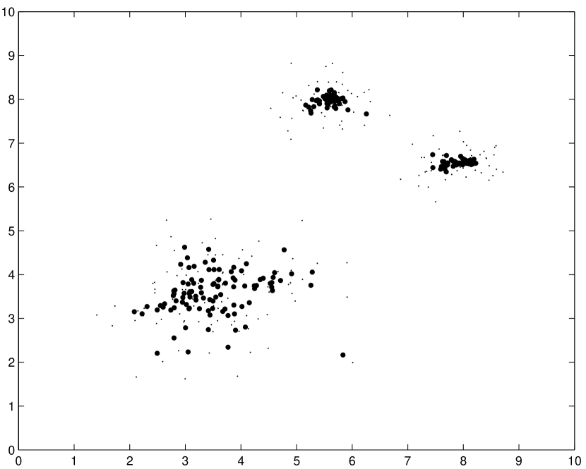
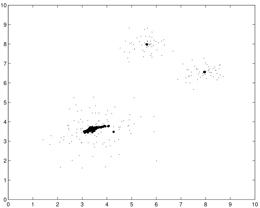
Figure 3: The positions of cluster centers (full circles): the left panel is after 1 iteration and the right panel is after 5 iterations. Please note that the original data points are indicated by dots.

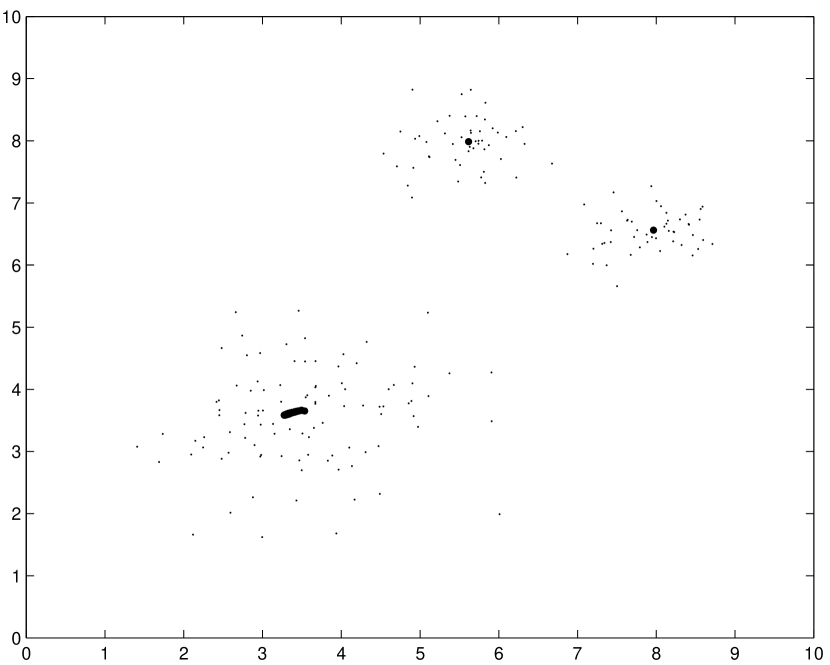
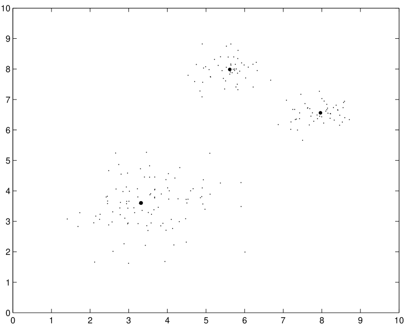
Figure 4: The positions of cluster centers (full circles): the left panel is after 10 iteration and the right panel is the convergent. Please note that the original data points are indicated by dots.

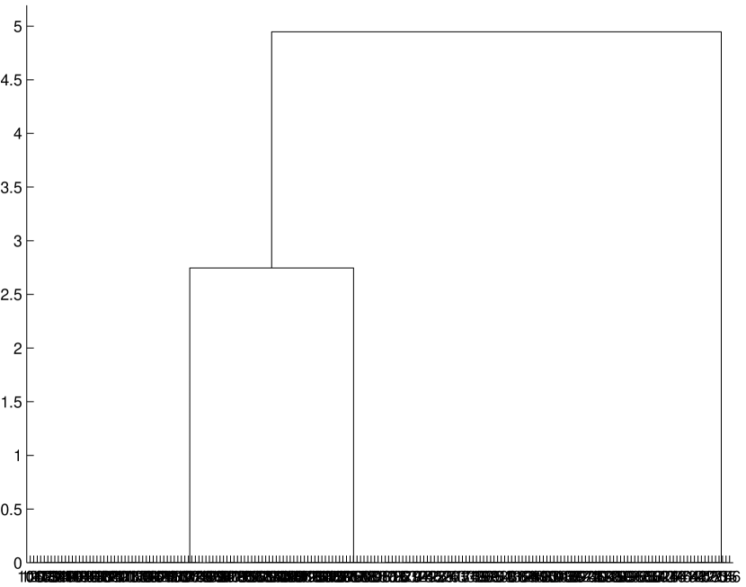
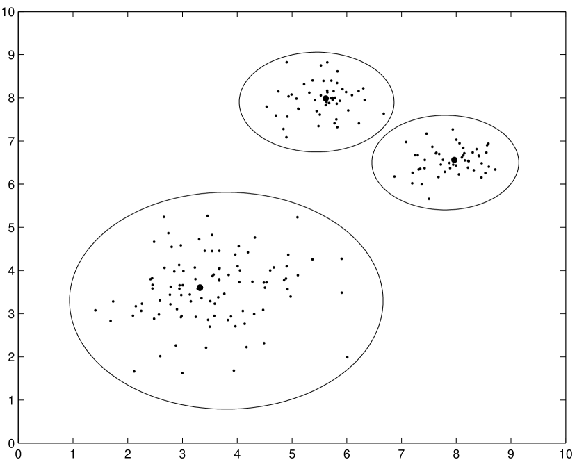
Figure 5: The left panel is the dendrogram through the SCM. There are too many data points, so the data identity numbers below the horizontal axis are not clear. The right panel is the identified clusters through the SCM.

Next, we present an example to illustrate the CCA and SCA. In the data set of Fig. 2, there are one large cluster and two small clusters. By the CCA, we find that $\gamma=10$ is a good estimate. Then we process SCA with this data set by initializing $z^{(0)}=(z_{1}^{(0)},\cdots,z_{n}^{(0)})=(x_{1},\cdots,x_{n})$. We show the positions of these cluster centers after 1, 5 and 10 iterations as the full circles in Fig. 3 and the left of Fig. 4, respectively. The final convergent positions of all cluster centers are shown as the full circles in the right of Fig. 4. Please note that all the data points, $(x_{1},\cdots,x_{n})$, are also plotted as the dots in Fig. 3 and 4. It is obvious that there are only three full circles because all cluster centers centralize to the three peaks of the SCM objective function. There are three clusters for this data set by the view of sight. However, a precise method to determine the cluster number from these final $n$ cluster centers should be provided. We use the single linkage algorithm with the final positions of all cluster centers to find the optimal cluster number $c^{*}$. The result is shown as the dendrogram in the left panel of Fig. 5. This dendrogram clearly indicates that there are three well separated clusters and hence the optimal cluster number $c^{*}=3$. At the same time the identified clusters will be found. The identified clusters are shown in the right panel of Fig. 5.

Therefore, we can completely cluster the data set in Fig. 2 into three clusters shown in the right panel of Fig. 5. The process includes that: (i) process CCA to estimate the parameter $\gamma$, (ii) process SCA with $z^{(0)}=(z_{1}^{(0)},\cdots,z_{n}^{(0)})=(x_{1},\cdots,x_{n})$, and (iii) process the single linkage algorithm with the final positions of $n$ cluster centers to find the optimal cluster number $c^{*}$ and identify these $c^{*}$ clusters. This forms the structure of SCM which is summarized as follows:

Similarity-Based Clustering Method (SCM)

• Estimate $\gamma$ using CCA;

• Process SCA with $z^{(0)}=(z_{1}^{(0)},\cdots,z_{n}^{(0)})=(x_{1},\cdots,x_{n})$;

• Process the single linkage algorithm with the final $n$ cluster centers;

• Find the optimal cluster number $c^{*}$ according to the dendrogram;

• Identify these $c^{*}$ clusters.

4 The Numerical Examples and Comparisons

In this section, we consider the bivariate normal mixtures of three classes in order to assess the performance of the single linkage algorithm and SCM. Let $N_{2}(\mathbf{a},\mathbf{\Sigma})$ represent the bivariate normal with mean vector $\mathbf{a}$ and covariance matrix $\mathbf{\Sigma}$, we consider the random sample of data drawn from

$$\alpha_{1}N_{2}({\mathbf{a}}_{1},{\mathbf{\Sigma}_{1}})+\alpha_{2}N_{2}({\mathbf{a}}_{2},{\mathbf{\Sigma}_{2}})+\alpha_{3}N_{2}({\mathbf{a}}_{3},{\mathbf{\Sigma}_{3}})$$

with $\alpha_{1}+\alpha_{2}+\alpha_{3}=1$, $0<\alpha_{i}<1,~{}i=1,2,3$. We design various bivariate normal mixture distributions shown in Table 1. In each test, we consider the sample size $n=200$.

Table 1. Various Bivariate Normal Mixture Distributions for the Three Tests

Test	$\alpha_{1}$	${\mathbf{a}}_{1}$	${\mathbf{\Sigma}_{1}}$	$\alpha_{2}$	${\mathbf{a}}_{2}$	${\mathbf{\Sigma}_{2}}$	$\alpha_{3}$	${\mathbf{a}}_{3}$	${\mathbf{\Sigma}_{3}}$
1	$0.2$	$(1,1)$	$\left(\begin{array}[]{cc}1.2&0\\ 0&1.2\end{array}\right)$	$0.3$	$(5.7,5.7)$	$\left(\begin{array}[]{cc}1&0\\ 0&1\end{array}\right)$	$0.5$	$(9,9)$	$\left(\par\begin{array}[]{cc}1.5&0\\ 0&1.5\end{array}\right)$
2	$0.2$	$(1,1)$	$\left(\begin{array}[]{cc}2&1.5\\ 1.5&2\end{array}\right)$	$0.3$	$(5,5)$	$\left(\begin{array}[]{cc}3&0.5\\ 0.5&3\end{array}\right)$	$0.5$	$(10,10)$	$\left(\begin{array}[]{cc}2&1\\ 1&2\end{array}\right)$
3	$0.2$	$(1,3)$	$\left(\begin{array}[]{cc}2&1.5\\ 1.5&4\end{array}\right)$	$0.3$	$(5,7)$	$\left(\begin{array}[]{cc}3&0.5\\ 0.5&5\end{array}\right)$	$0.5$	$(9,11)$	$\left(\begin{array}[]{cc}6&1\\ 1&4\end{array}\right)$

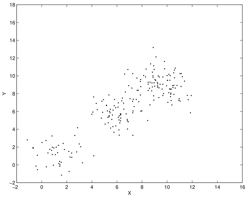
Figure 6: The data set generated for Test 1

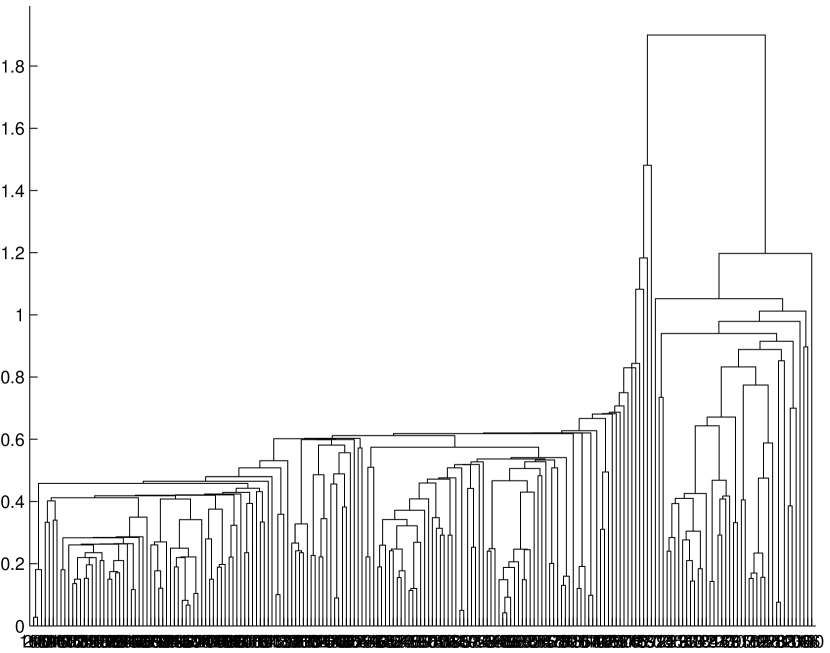
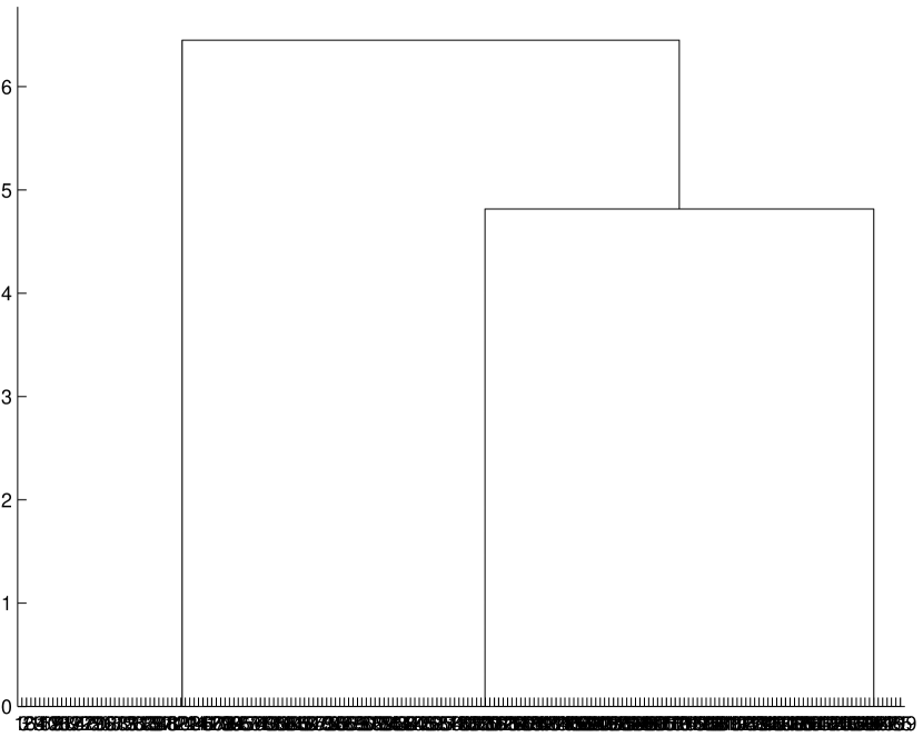
Figure 7: The dendrogram of Test 1: the single linkage algorithm’s result is on the left and the SCM’s is on the right. There are too many data points, so the data identity numbers below the horizontal axis are not clear.

The data set generated for Test 1 is shown in Fig. 6. From Fig. 6, it seems there are 2 or 3 clusters. Thus, a precise method to determine the cluster number is necessary. We process the single linkage algorithm and SCM with this data set. The clustering results are shown in Fig. 7. In the left panel, it is clear that different cut-off level of distances would give different number of clusters for the single linkage algorithm’s result. In the right panel of Fig. 7, SCM clearly indicates that there are three well-separated clusters. Furthermore, the cluster centers are $(1.2784,1.3323),(5.9372,5.7933),(9.4804,9.0544)$. These results reflect the original structure of the data set designed for Test 1.

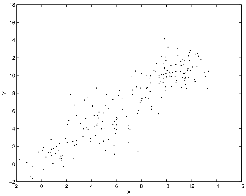
Figure 8: The data set generated for Test 2

Fig. 8 shows the data set generated for Test 2. From Fig. 8, the cluster number seems to be 3. In the same way, we implement the single linkage algorithm and SCM on this data set. The dendrogram of the single linkage algorithm cannot classify this data set well. But the SCM clearly indicates that there are three well-separated clusters. Furthermore, the cluster centers are $(1.2096,1.3824),(4.9835,4.6876),(10.6420,10.3181)$. These results reflect the structure of the data set designed for Test 2.

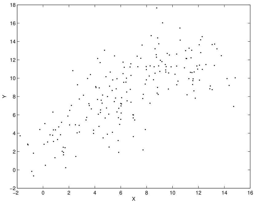
Figure 10: The data set generated for Test 3

Fig. 10 shows the data set generated for Test 3. It is difficult to know the cluster number from Fig. 10. We also implement the single linkage algorithm and SCM on this data set. The dendrogram of the single linkage algorithm looks very complicated. However, the SCM clearly indicates that there are three well-separated clusters. Furthermore, the cluster centers are $(1.2373,3.8693),(5.3338,7.2524),(9.3596,11.2041)$. These results reflect the original structure of the data set designed for Test 3.

For all the above three tests, SCM gave the optimal cluster number $c^{*}=3$ which is exactly the actual cluster number but the single linkage algorithm fails. It shows the superiority of SCM over the single linkage algorithm. As supported by these experiments, SCM produces satisfactory results with the artificially generated data.

5 The Results

In this section, both the single linkage algorithm and the SCM will be used to cluster the data of extrasolar planets. Our data is from the Extrasolar Planets Catalog maintained by Jean Schneider (http://cfa-www.harvard.edu/planets/catalog.html). We use the data of April 2005 and exclude the incomplete ones. There are 143 planets (see the Appendix) available for our work and each of them have the values of $M{\rm sin}~{}i$, orbital period $P$, semi-major axis $a$ and also orbital eccentricity $e$, where $M$ is the planetary mass and $i$ is the unknown orbital inclinations. We set ${\rm sin}~{}i$ = 1, for simplicity (Trilling et al. 2002). This assumption shall not have a significant impact on the results of our clustering analysis because it is not the absolute mass that matters but the structures of the mass distribution.

5.1 The Planetary Masses and Periods

Since there is a possible mass-period correlation for extrasolar planets (Zucker & Mazeh 2002, Pätzold & Rauer 2002, Jiang et al. 2003), it should be interesting to see whether there are groups for extrasolar planets on the ${\rm ln}P$-${\rm ln}M$ plane. The results of this clustering analysis would give hints about the formation conditions of these planets.

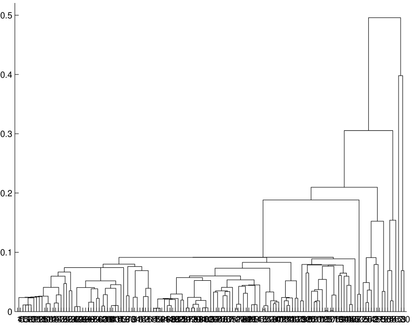
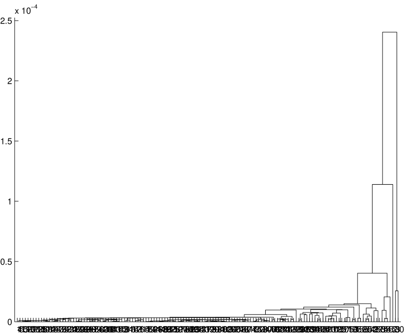
Figure 12: The dendrogram of exoplanets in the ${\rm ln}M$ space: the single linkage algorithm’s result is on the left and the SCM’s is on the right. There are too many data points, so the data identity numbers below the horizontal axis are not clear.

To investigate the problem step by step, we first study the possible clustering on the space of ${\rm ln}M$. The dendrogram illustrating the hierarchical clustering for ${\rm ln}M$ space is shown in the left panel of Fig. 12. From the dendrogram, we find that clustering (or mergers) takes place at different levels. For example, there are two clusters with the distance of about 0.48. One of them can actually be divided into two with the distance of about 0.38. Thus, the number of clusters keeps increasing and becomes very large when a smaller distance is chosen as the condition to group the data. Consequently, it is difficult to identity the final configuration of clusters. Please note that because there are too many data points, the data identity numbers below the horizontal axis of all dendrograms in this section are not clear. They can be ignored here. To obtain a better partition for this data, we use the SCM to do the analysis. The corresponding dendrogram is shown in the right panel of Fig. 12. From this dendrogram, the vertical axis indicates that the largest level is at $2.4\times 10^{-4},$ which is less than our chosen $\epsilon$ in SCA (We set $\epsilon=0.001$.). It means that the minimum distance between pairs of clusters is negligible. Therefore, all objects are merged to form a single cluster. That is, by SCM, the data of discovered exoplanets shall be regarded as a continuous distribution in the $\rm{ln}M$ space.

Indeed, the histogram of the exoplanets in the $\rm{ln}M$ space in Fig. 13 indicates that there is only one strong peak around ${\ln}M=0$ and the whole distribution seems to be continuous. Thus, the Jupiter-mass exoplanets dominate the population. Of course, there are many factors that influence the mass distribution. For example, the observational selection effect and perhaps also the orbital instability of close-in massive planets. Nevertheless, the clustering result showing there is only one group statistically confirms that there is no particular constraint on the possible planetary masses except their boundaries, i.e. the maximum and minimum masses.

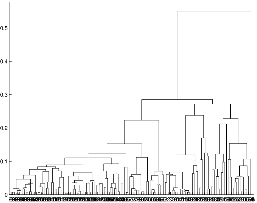
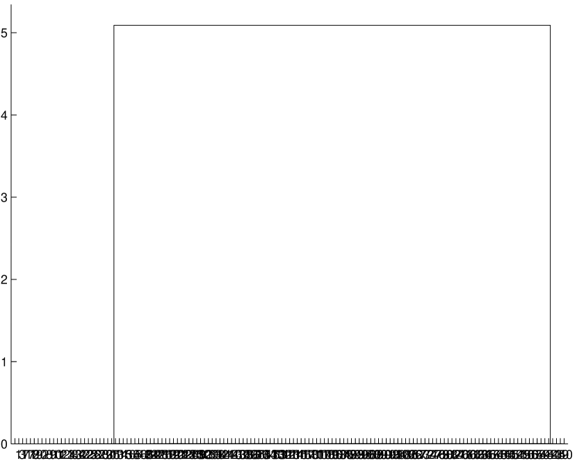
Figure 14: The dendrogram of exoplanets in the ${\rm ln}P$ space: the single linkage algorithm’s result is on the left and the SCM’s is on the right. There are too many data points, so the data identity numbers below the horizontal axis are not clear.

We then study the clustering on the ${\rm ln}P$ space. In the same way, we implement both the single linkage algorithm and SCM in the ${\rm ln}P$ space. The left and right panels of Fig. 14 show the dendrogram of these two methods, respectively. From the left panel of Fig. 14, there are no meaningful well-separated clusters. But there are two well-separated clusters in the right panel of Fig. 3. Thus, the SCM shows that there are 2 clusters, and the corresponding clustering results are shown in Table 2. The cluster with smaller average value of ${\rm ln}P$ is called Cluster $P_{1}$ and the other one is called Cluster $P_{2}$. The center of Cluster $P_{1}$ is at 1.4552 and the center of Cluster $P_{2}$ is at 6.5455.

Table 2. The clustering results in the ${\rm ln}P$ space.

Cluster	data point no.
$P_{1}$	1	2	3	4	7	8	9	10	11	12
	13	14	15	16	17	18	19	20	21	22
	25	26	27	28	29	30	33	34	35	37
	38
$P_{2}$	5	6	23	24	31	32	36	39	40	41
	42	43	44	45	46	47	48	49	50	51
	52	53	54	55	56	57	58	59	60	61
	62	63	64	65	66	67	68	69	70	71
	72	73	74	75	76	77	78	79	80	81
	82	83	84	85	86	87	88	89	90	91
	92	93	94	95	96	97	98	99	100	101
	102	103	104	105	106	107	108	109	110	111
	112	113	114	115	116	117	118	119	120	121
	122	123	124	125	126	127	128	129	130	131
	132	133	134	135	136	137	138	139	140	141
	142	143

We also make a histogram of our data in the ${\rm ln}P$ space. As shown in Fig. 15, for this case, it is difficult to group the data by eye. The two crosses in Fig. 15 indicate the cluster centers determined by SCM. They are very close to the peaks of the histogram, so the result of SCM is indeed reasonable and correct. Thus, we have statistically shown that there are two clusters for exoplanets in the ${\rm ln}P$ space. The distribution of orbital periods is unlikely to be a continuous function. In fact, there is a statistical gap between two continuous distributions.

How could that gap form? There could be two possibilities: (1) it is difficult to form the planets at particular distances from the central stars, (2) planetary migrations did happen. The possible planetary migrations as studied in many theoretical papers are good candidates to affect the results of observed period distribution. However, if there is only one migration mechanism, the resulting distribution is probably still continuous, unless that the rate of this migration mechanism varies as a sharp function of the orbital period. If there is a period for which the migration rate is fastest, we might expect much less systems would end up there. Another simple interpretation is that there are two important migration mechanisms to make the exoplanets have two clusters in the ${\rm ln}P$ space. Indeed, the center of Cluster $P_{1}$, 1.4552, is within the regime in which the tidal interaction with the central star is important (Jiang et al. 2003) and the center of Cluster $P_{2}$, 6.5455, is within the regime in which the disc interaction is important (Armitage et al. 2002, Trilling et al. 2002). The migrations caused by these two mechanisms, tidal interaction and disc interaction, might produce the two clusters in our statistical results.

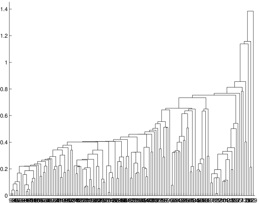
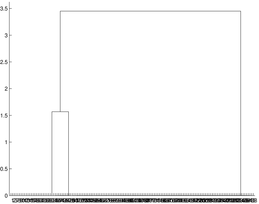
Figure 16: The dendrogram of exoplanets in the ${\rm ln}P-{\rm ln}M$ space: the single linkage algorithm’s result is on the left and the SCM’s is on the right. There are too many data points, so the data identity numbers below the horizontal axis are not clear.

Next, we consider the clustering on the ${\rm ln}P$-${\rm ln}M$ space. In the same way, we implement both the single linkage algorithm and the SCM on the data in the ${\rm ln}P$-${\rm ln}M$ space. Fig. 16 shows the dendrogram of these two methods. The right panel of Fig. 16 clearly indicates that there are three well-separated clusters. Three clusters are called Cluster $PM_{1}$, $PM_{2}$ and $PM_{3}$ and their centers are at $({\rm ln}P,{\rm ln}M)=(1.2750,-0.6980)$, $(2.8093,-0.3710)$ and $(6.1522,0.4857)$, respectively. Table 3 shows the members of these three clusters.

Table 3. The clustering results in the ${\rm ln}P$-${\rm ln}M$ space.

Cluster	data point no.
$PM_{1}$	1	2	3	7	8	9	10	11	12	13
	14	15	16	17	18	19	20	21	22	25
	26	27	28	30	33	34
$PM_{2}$	4	29	35	37	39	40	41	42	43	48
$PM_{3}$	5	6	23	24	31	32	36	38	44	45
	46	47	49	50	51	52	53	54	55	56
	57	58	59	60	61	62	63	64	65	66
	67	68	69	70	71	72	73	74	75	76
	77	78	79	80	81	82	83	84	85	86
	87	88	89	90	91	92	93	94	95	96
	97	98	99	100	101	102	103	104	105	106
	107	108	109	110	111	112	113	114	115	116
	117	118	119	120	121	122	123	124	125	126
	127	128	129	130	131	132	133	134	135	136
	137	138	139	140	141	142	143

Fig. 17 shows the distribution of exoplanet in the ${\rm ln}P$-${\rm ln}M$ space. The triangles are the members of Cluster $PM_{1}$, the open squares are the members of Cluster $PM_{2}$, and the full circles are the members of Cluster $PM_{3}$. There are two are reasons for the crosses going from the bottom-left to the top-right. The observational selection effect explains the absence in the bottom-right corner and the tidal interaction (Jiang et al. 2003) explains the absence in the top-left corner.

It is not surprising that there are more than one cluster here as there are already two clusters in the ${\rm ln}P$ space. From Fig. 15 and 17, we can see that Cluster $PM_{1}$ is very much overlapping Cluster $P_{1}$ and Cluster $PM_{3}$ is overlapping Cluster $P_{2}$. The reason why the Cluster $PM_{2}$ exists is that there is a very massive close-in planet, HD 162020 b (data 29), with mass ($Msini$) 13.75 $M_{J}$ and period 8.42 days. This planet together with a few other massive close-ins stand out as a new class. If some of the members of Cluster $PM_{2}$ fall into the central stars and thus disappear in the plot, this cluster might be absorbed by the other two clusters. Cluster $PM_{2}$ might represent the temporary group with members falling into the stars in the near future. Thus, we speculate that this cluster experiences on-going tidal interaction.

5.2 Orbital Eccentricities

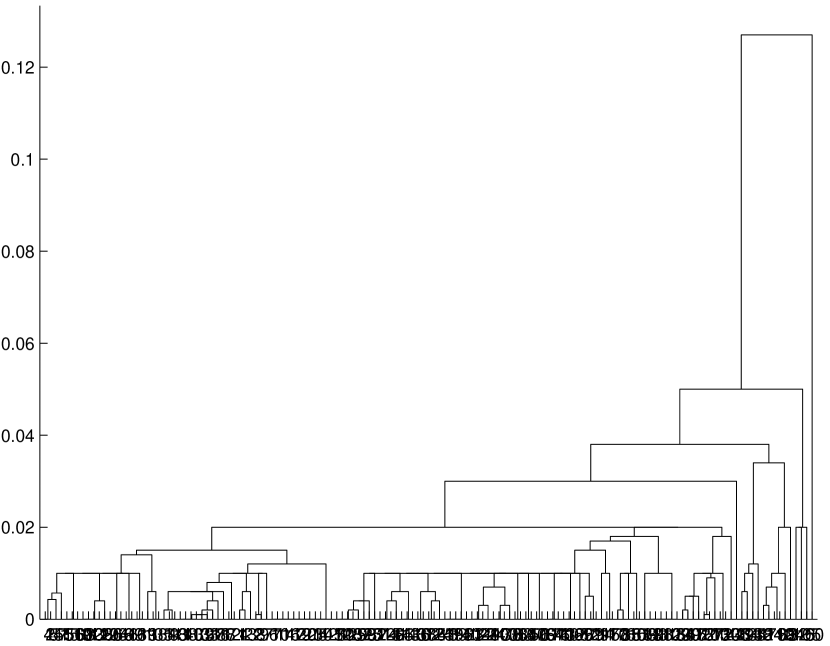
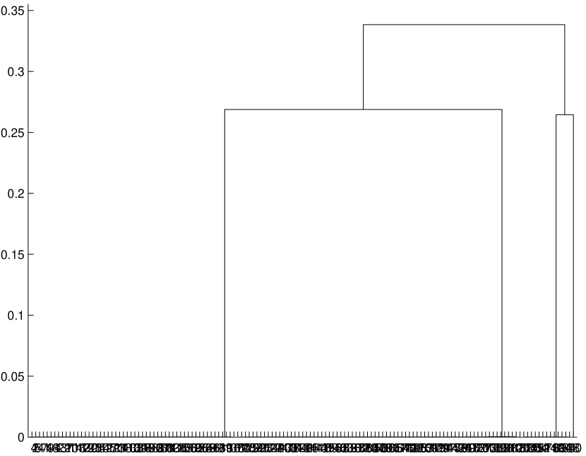
Figure 18: The dendrogram of exoplanets in the $e$ space: the single linkage algorithm’s result is on the left and the SCM’s is on the right. There are too many data points, so the data identity numbers below the horizontal axis are not clear.

To understand more about the orbital properties of these exoplanets, we study the possible clustering in the eccentricity $e$ space. We shall also study the clustering of exoplanets’ semi-major axes. Because ${\rm ln}a$ is simply a constant times ${\rm ln}P$, the clustering of the data in the ${\rm ln}a$ space is the same as in the ${\rm ln}P$ space. Thus, we use ${\rm ln}P$ to represent ${\rm ln}a$ and study the clustering in the ${\rm lnP}-e$ space. In the same way, we implement the single linkage algorithm and SCM on the data in the $e$ space. Fig. 18 shows the resulting dendrogram by these two methods. The right panel of Fig. 18 clearly indicates that there are four well-separated clusters but the left panel fails. Therefore, the SCM shows that there are 4 clusters, and the corresponding clustering results are shown in Table 4. Furthermore, the cluster centers of Cluster $e_{1}$, $e_{2}$, $e_{3}$, and $e_{4}$ are at 0.0486, 0.3177, 0.6562, and 0.9207, respectively.

Table 4. The clustering result in the $e$ space.

Cluster	data point no.
$e_{1}$	1	2	3	4	6	7	8	9	10	11
	12	13	14	15	16	17	18	19	20	21
	22	25	26	27	28	30	33	37	38	39
	40	42	44	45	46	48	55	56	57	66
	68	71	88	96	99	102	111	113	118	119
	120	135	136	139
$e_{2}$	5	23	24	29	31	34	35	36	41	43
	47	50	52	53	58	59	61	62	63	64
	65	67	70	72	73	74	75	76	77	78
	80	81	82	83	84	85	86	87	89	90
	91	92	93	94	95	97	98	100	101	103
	106	107	108	109	110	114	116	117	121	122
	123	125	126	127	128	129	130	131	132	133
	137	140	141	142	143
$e_{3}$	32	49	51	54	69	79	104	105	112	115
	124	134	138
$e_{4}$	60

We also plot the histogram of the data in the $e$ space as shown in Fig. 19. From the histogram, it looks as though there is more than one cluster but it is difficult to determine the number of clusters by eye. The result of SCM seems to be reasonable, particularly after we add the crosses to indicate the centers of these four clusters. Even though there are four clusters in the $e$ space, there is only one member in the Cluster $e_{4}$ and this planet has a very large orbital eccentricity 0.927.

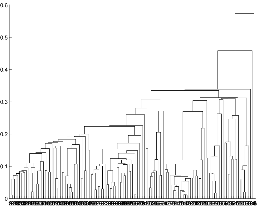
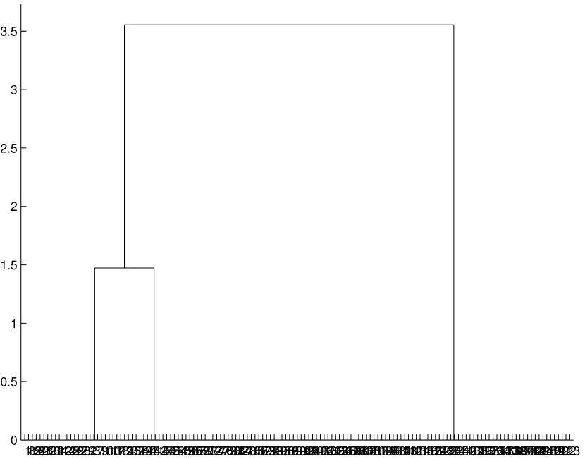
Figure 20: The dendrogram of exoplanets in the ${\rm ln}P-e$ space: the single linkage algorithm’s result is on the left and the SCM’s is on the right. There are too many data points, so the data identity numbers below the horizontal axis are not clear.

Finally, we consider the single linkage algorithm and the SCM in the ${\rm ln}P-e$ space. In the same way, we implement the single linkage algorithm and SCM on the data. The left and right panels of Fig. 20 show the dendrogram of these two methods, respectively. The right panel clearly indicates that there are three well-separated clusters. Table 5 shows the SCM’s clustering results. The cluster centers of Cluster $Pe_{1}$, $Pe_{2}$, and $Pe_{3}$ are given by $({\rm ln}P,e)=(1.2860,0.0446)$, $(2.7573,0.1206)$, and $(6.3061,0.3396)$, respectively.

Table 5. The clustering results in the ${\rm ln}P-e$ space.

Cluster	data point no.
$Pe_{1}$	1	2	3	7	8	9	10	11	12	13
	14	15	16	17	18	19	20	21	22	25
	26	27	28	29	30	33	34
$Pe_{2}$	4	35	37	38	39	40	41	42	45
$Pe_{3}$	5	6	23	24	31	32	36	43	44	46
	47	48	49	50	51	52	53	54	55	56
	57	58	59	60	61	62	63	64	65	66
	67	68	69	70	71	72	73	74	75	76
	77	78	79	80	81	82	83	84	85	86
	87	88	89	90	91	92	93	94	95	96
	97	98	99	100	101	102	103	104	105	106
	107	108	109	110	111	112	113	114	115	116
	117	118	119	120	121	122	123	124	125	126
	127	128	129	130	131	132	133	134	135	136
	137	138	139	140	141	142	143

In the ${\rm ln}P-e$ space as shown in Fig. 21, there are two data points in Cluster $Pe_{2}$ with a particularly large $e$ and thus form a class. They are data 35 and data 41. We find that these two are also in the Cluster $PM_{2}$, so they are likely to be the temporary cluster, in which some of the members will fall into their central stars in the near future. In general, the exoplanet data in the ${\rm ln}P-e$ space shows that there is a strong eccentricity-period correlation. That is, the planets with larger orbital periods might have larger eccentricities.

6 Speculations and Implications

To statistically investigate the properties of the distributions of the mass, period, and orbits of exoplanets, we have used both the conventional method, single-linkage algorithm, and the advanced SCM of Cluster Analysis to study the possible clusters of the exoplanets in the ${\rm ln}M$, ${\rm ln}P$, ${\rm ln}P-{\rm ln}M$, $e$, and ${\rm ln}P-e$ space. In general, the SCM gives very good and reasonable results.

We find that there is only one cluster in the ${\rm ln}M$ space, so a continuous mass function (Tabachnik and Tremaine 2002) would be a good approximation. We find that there are two clusters in the ${\rm ln}P$ space and this could be due to two migration mechanisms; tidal and disc interactions. In addition to the two clusters associated with the above two mechanisms, there is one more cluster which might present the massive close-in exoplanets with on-going tidal interaction in the ${\rm ln}P-{\rm ln}M$ space. Our SCM found that there are four clusters in the $e$ space. However, there is only one member in the Cluster $e_{4}$, which is an unusual case with an extremely large eccentricity 0.927. The other three clusters, Cluster $e_{1}$, $e_{2}$, and $e_{3}$ might associate with the tidal, on-going tidal, and disc interactions, respectively. The three clusters in the ${\rm ln}P-e$ space, Cluster $Pe_{1}$, $Pe_{2}$, and $Pe_{3}$ could associate with the same things, respectively. Finally, the eccentricity-period correlation is strong and obvious.

Figure 1: The dendrogram for distances between five objects in the example of Section 2.

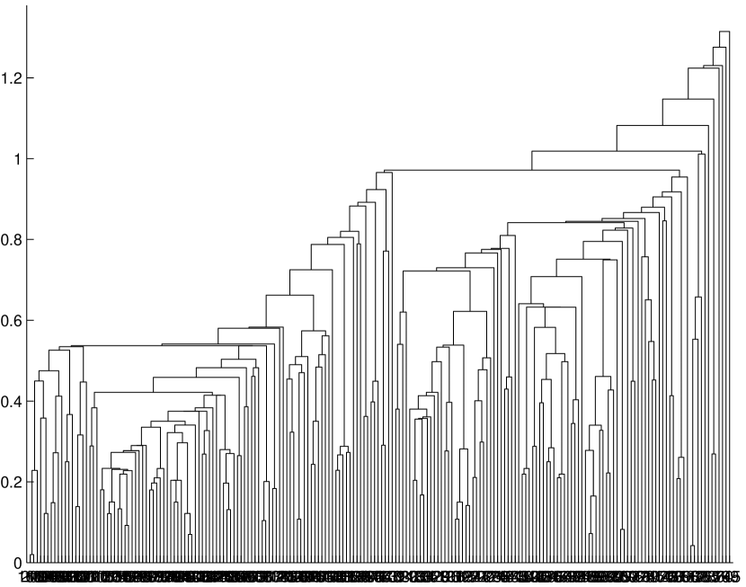
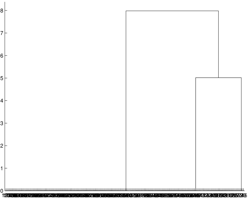
Figure 9: The dendrogram of Test 2: the single linkage algorithm’s result is on the left and the SCM’s is on the right. There are too many data points, so the data identity numbers below the horizontal axis are not clear.

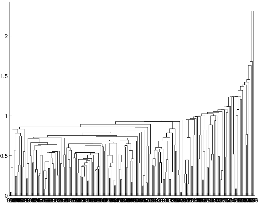
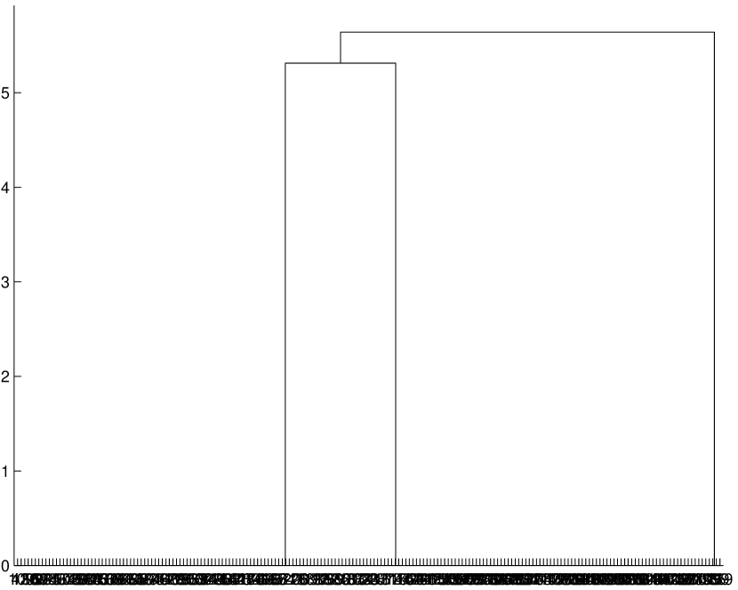
Figure 11: The dendrogram of Test 3: the single linkage algorithm’s result is on the left and the SCM’s is on the right. There are too many data points, so the data identity numbers below the horizontal axis are not clear.

Figure 13: The histogram of exoplanets in the ${\rm ln}M$ space.

Figure 15: The histogram of exoplanets in the ${\rm ln}P$ space. In the plot, the left cross indicates that the center of Cluster $P_{1}$ is at 1.4552 and the right cross indicates that the center of Cluster $P_{2}$ is at 6.5455.

Figure 17: The distribution of exoplanets in the ${\rm ln}P-{\rm ln}M$ space. There are three crosses indicating the centers of three clusters. The triangles indicate the members of the Cluster $PM_{1}$, the open squares indicate the members of the Cluster $PM_{2}$, and the full circles indicate the members of the Cluster $PM_{3}$.

Figure 19: The histogram of exoplanets in the $e$ space. There are four crosses indicating the centers of four clusters.

Figure 21: The distribution of exoplanets in the ${\rm ln}P-e$ space. There are three crosses indicating the centers of three clusters. The triangles indicate the members of the Cluster $Pe_{1}$, the open squares indicate the members of the Cluster $Pe_{2}$, and the full circles indicate the members of the Cluster $Pe_{3}$.

Appendix

Extra-solar planets data

No.	NAME	M[.SINI]	SEM-MAJ.AXIS	PERIOD	ECC
		Jup. mass	(AU)	days
1	HD 73256 b	1.85	0.037	2.54863	0.038
2	GJ 436 b	0.067	0.0278	2.6441	0.12
3	55 Cnc e	0.045	0.038	2.81	0.174
4	55 Cnc b	0.84	0.11	14.65	0.02
5	55 Cnc c	0.21	0.24	44.28	0.34
6	55 Cnc d	4.05	5.9	5360	0.16
7	HD 63454 b	0.38	0.036	2.81782	0
8	HD 83443 b	0.41	0.04	2.985	0.08
9	HD 46375 b	0.249	0.041	3.024	0.04
10	TrES-1	0.75	0.0393	3.030065	0
11	HD 179949 b	0.84	0.045	3.093	0.05
12	HD 187123 b	0.52	0.042	3.097	0.03
13	Tau Boo b	3.87	0.0462	3.3128	0.018
14	HD 330075 b	0.76	0.043	3.369	0
15	HD 88133 b	0.29	0.046	3.415	0.11
16	HD 2638 b	0.48	0.044	3.4442	0
17	BD-10 3166 b	0.48	0.046	3.487	0
18	HD 75289 b	0.42	0.046	3.51	0.054
19	HD 209458 b	0.69	0.045	3.52474541	0
20	HD 76700 b	0.197	0.049	3.971	0
21	51 Peg b	0.468	0.052	4.23077	0
22	Ups And b	0.69	0.059	4.617	0.012
23	Ups And c	1.19	0.829	241.5	0.28
24	Ups And d	3.75	2.53	1284	0.27
25	HD 49674 b	0.12	0.0568	4.948	0
26	HD 68988 b	1.9	0.071	6.276	0.14
27	HD 168746 b	0.23	0.065	6.403	0.081
28	HD 217107 b	1.28	0.07	7.11	0.14
29	HD 162020 b	13.75	0.072	8.428198	0.277
30	HD 160691 d	0.042	0.09	9.55	0

(Continued) Extra-solar planets data

No.	NAME	M[.SINI]	SEM-MAJ.AXIS	PERIOD	ECC
		Jup. mass	(AU)	days
31	HD 160691 b	1.7	1.5	638	0.31
32	HD 160691 c	3.1	4.17	2986	0.8
33	HD 130322 b	1.08	0.088	10.724	0.048
34	HD 108147 b	0.41	0.104	10.901	0.498
35	HD 38529 b	0.78	0.129	14.309	0.29
36	HD 38529 c	12.7	3.68	2174.3	0.36
37	Gl 86 b	4	0.11	15.78	0.046
38	HD 99492 b	0.112	0.119	17.038	0.05
39	HD 27894 b	0.62	0.122	17.991	0.049
40	HD 195019 b	3.43	0.14	18.3	0.05
41	HD 6434 b	0.48	0.15	22.09	0.3
42	HD 192263 b	0.72	0.15	24.348	0
43	Gliese 876 c	0.56	0.13	30.1	0.27
44	Gliese b	1.98	0.21	61.02	0.12
45	HD 102117 b	0.14	0.149	20.67	0
46	HD 11964 c	0.11	0.23	37.82	0.15
47	HD 11964 b	0.7	3.17	1940	0.3
48	rho CrB b	1.04	0.22	39.845	0.04
49	HD 74156 b	1.86	0.294	51.643	0.636
50	HD 117618 b	0.19	0.28	52.2	0.39
51	HD 37605 b	2.4	0.26	55.02	0.677
52	HD 168443 b	7.7	0.29	58.116	0.529
53	HD 168443 c	16.9	2.85	1739.5	0.228
54	HD 3651 b	0.2	0.284	62.23	0.63
55	HD 121504 b	0.89	0.32	64.6	0.13
56	HD 101930 b	0.3	0.302	70.46	0.11
57	HD 178911 B b	6.292	0.32	71.487	0.1243
58	HD 16141 b	0.23	0.35	75.56	0.21
59	HD 114762 b	11	0.3	84.03	0.334
60	HD 80606 b	3.41	0.439	111.78	0.927

(Continued) Extra-solar planets data

No.	NAME	M[.SINI]	SEM-MAJ.AXIS	PERIOD	ECC
		Jup. mass	(AU)	days
61	70 Vir b	7.44	0.48	116.689	0.4
62	HD 216770 b	0.65	0.46	118.45	0.37
63	HD 52265 b	1.13	0.49	118.96	0.29
64	HD 34445 b	0.58	0.51	126.	0.4
65	HD 208487 b	0.45	0.49	130	0.32
66	HD 93083 b	0.37	0.477	143.58	0.14
67	GJ 3021 b	3.21	0.49	133.82	0.505
68	HD 37124 b	0.75	0.54	152.4	0.1
69	HD 37124 c	1.2	2.5	1495	0.69
70	HD 73526 b	3	0.66	190.5	0.34
71	HD 104985 b	6.3	0.78	198.2	0.03
72	HD 82943 b	0.88	0.73	221.6	0.54
73	HD 82943 c	1.63	1.16	444.6	0.41
74	HD 169830 b	2.88	0.81	225.62	0.31
75	HD 169830 c	4.04	3.6	2102	0.33
76	HD 8574 b	2.23	0.76	228.8	0.4
77	HD 202206 b	17.4	0.883	225.87	0.435
78	HD 202206 c	2.44	2.55	1383.4	0.267
79	HD 89744 b	7.99	0.89	256.6	0.67
80	HD 134987 b	1.58	0.78	260	0.25
81	HD 40979 b	3.32	0.811	267.2	0.25
82	HD 12661 b	2.3	0.83	263.6	0.35
83	HD 12661 c	1.57	2.56	1444.5	0.2
84	HD 150706 b	1	0.82	264.9	0.38
85	HR 810 b	1.94	0.91	311.288	0.24
86	HD 142 b	1.36	0.98	338	0.37
87	HD 92788 b	3.8	0.94	340	0.36
88	HD 28185 b	5.6	1	385	0.06
89	HD 196885 b	1.84	1.12	386	0.3
90	HD 142415 b	1.62	1.05	386.3	0.5

(Continued) Extra-solar planets data

No.	NAME	M[.SINI]	SEM-MAJ.AXIS	PERIOD	ECC
		Jup. mass	(AU)	days
91	HD 177830 b	1.28	1	391	0.43
92	HD 154857 b	1.8	1.11	398	0.51
93	HD 108874 b	1.65	1.07	401	0.2
94	HD 4203 b	1.65	1.09	400.944	0.46
95	HD 128311 b	2.58	1.02	420	0.3
96	HD 27442 b	1.28	1.18	423.841	0.07
97	HD 210277 b	1.28	1.097	437	0.45
98	HD 19994 b	2	1.3	454	0.2
99	HD 188015 b	1.26	1.19	456.46	0.15
100	HD 13189 b	14	1.85	471.6	0.27
101	HD 20367 b	1.07	1.25	500	0.23
102	HD 114783 b	0.9	1.2	501	0.1
103	HD 147513 b	1	1.26	540.4	0.52
104	HIP 75458 b	8.64	1.34	550.651	0.71
105	HD 222582 b	5.11	1.35	572	0.76
106	HD 65216 b	1.21	1.37	613.1	0.41
107	HD 183263 b	3.69	1.52	634.23	0.38
108	HD 141937 b	9.7	1.52	653.22	0.41
109	HD 41004A b	2.3	1.31	655	0.39
110	HD 47536 b	7.32	1.93	712.13	0.2
111	HD 23079 b	2.61	1.65	738.459	0.1
112	16 CygB b	1.69	1.67	798.938	0.67
113	HD 4208 b	0.8	1.67	812.197	0.05
114	HD 114386 b	0.99	1.62	872	0.28
115	HD 45350 b	0.98	1.77	890.76	0.78
116	gamma Cephei b	1.59	2.03	902.96	0.2
117	HD 213240 b	4.5	2.03	951	0.45
118	HD 10647 b	0.91	2.1	1040	0.18
119	HD 10697 b	6.12	2.13	1077.906	0.11
120	47 Uma b	2.41	2.1	1095	0.096

(Continued) Extra-solar planets data

No.	NAME	M[.SINI]	SEM-MAJ.AXIS	PERIOD	ECC
		Jup. mass	(AU)	days
121	HD 190228 b	4.99	2.31	1127	0.43
122	HD 114729 b	0.82	2.08	1131.478	0.31
123	HD 111232 b	6.8	1.97	1143	0.2
124	HD 2039 b	4.85	2.19	1192.582	0.68
125	HD 136118 b	11.9	2.335	1209.6	0.366
126	HD 50554 b	4.9	2.38	1279	0.42
127	HD 196050 b	3	2.5	1289	0.28
128	HD 216437 b	2.1	2.7	1294	0.34
129	HD 216435 b	1.49	2.7	1442.919	0.34
130	HD 106252 b	6.81	2.61	1500	0.54
131	HD 23596 b	7.19	2.72	1558	0.314
132	14 Her b	4.74	2.8	1796.4	0.338
133	HD 142022	4.4	2.8	1923	0.57
134	HD 39091 b	10.35	3.29	2063.818	0.62
135	HD 72659 b	2.55	3.24	2185	0.18
136	HD 70642 b	2	3.3	2231	0.1
137	HD 33636 b	9.28	3.56	2447.292	0.53
138	Epsilon Eridanib	0.86	3.3	2502.1	0.608
139	HD 117207 b	2.06	3.78	2627.08	0.16
140	HD 30177 b	9.17	3.86	2819.654	0.3
141	HD 50499 b	1.84	4.403	2990	0.32
142	Gl 777A b	1.33	4.8	2902	0.48
143	HD 89307 b	2.73	4.15	3090	0.32

References

- (1) Armitage, P. J., Livio, M., Lubow, S. H., Pringle, J. E., 2002, MNRAS, 334, 248
- (2) Baggaley, W. J., Galligan, D. P., 1997, Planetary and Space Science, 45, 865
- (3) Galligan, D. P., 2003a, MNRAS, 340, 893
- (4) Galligan, D. P., 2003b, MNRAS, 340, 899
- (5) Gower, J. C., Ross, G. J. S., 1969, Appl. Stat., 18, 54
- (6) Hartigan, J.A., 1967, J. Am. Stat. Ass., 62, 1140
- (7) Hartigan, J.A., 1975, Clustering Algorithms (Wiley, New York)
- (8) Ji, J., Kinoshita, H., Liu, L., Li, G. 2003, ApJ, 585, L139
- (9) Ji, J., Li, G., Liu, L. 2002, ApJ, 572, 1041
- (10) Jiang, I.-G., Ip, W.-H., 2001, A&A, 367, 943
- (11) Jiang, I.-G., Ip, W.-H., Yeh, L.-C., 2003, ApJ, 582, 449
- (12) Jiang, I.-G., Yeh, L.-C. 2004a, AJ, 128, 923
- (13) Jiang, I.-G., Yeh, L.-C. 2004b, Int. J. Bifurcation and Chaos, 14, 3153
- (14) Johnson, R. A., Wichern, D. W., 1988, Applied Multivariate Statistical Analysis (Prentice-Hall, Inc.)
- (15) MacQueen, J., 1967, Proceeding of the Fifth Berkeley Symposium on Mathematical Statistics and Probability (University of California Press, Berkeley), 281
- (16) Pätzold, M., Rauer, H., 2002, ApJ, 568, L117
- (17) Tabachnik, S., Tremaine, S., 2002, MNRAS, 335, 151
- (18) Trilling, D. E., Lunine, J. I., Benz, W., 2002, A&A, 394, 241
- (19) Veras, D., Armitage, P. J., 2004, MNRAS, 347, 613
- (20) Yang, M.-S., Wu, K.-L., 2004, IEEE Trans. PAMI, 26, 434
- (21) Yeh, L.-C., Jiang, I.-G., 2001, ApJ, 561, 364
- (22) Zakamska, N. L., Tremaine, S., 2004, AJ, 128, 869
- (23) Zappala, V., Bendjoya, P., Cellino, A., Farinella, P., Froeschle, C., 1995, Icarus, 116, 291
- (24) Zucker, S., Mazeh, T., 2002, ApJ, 568, L113