X-ray and TeV Gamma-Ray Emission from Parallel Electron-Positron or Electron-Proton Beams in BL Lac Objects

Abstract

In this paper we discuss models of the X-rays and TeV $\gamma$-ray emission from BL Lac objects based on parallel electron-positron or electron-proton beams that form close to the central black hole owing to the strong electric fields generated by the accretion disk and possibly also by the black hole itself. Fitting the energy spectrum of the BL Lac object Mrk 501, we obtain tight constraints on the beam properties. Launching a sufficiently energetic beam requires rather strong magnetic fields close to the black hole ($\sim 100-1000$ G). However, the model fits imply that the magnetic field in the emission region is only $\sim 0.02$ G. Thus, the particles are accelerated close to the black hole and propagate a considerable distance before instabilities trigger the dissipation of energy through synchrotron and self-Compton emission. We discuss various approaches to generate enough power to drive the jet and, at the same time, to accelerate particles to $\sim$20 TeV energies. Although the parallel beam model has its own problems, it explains some of the long-standing problems that plague models based on Fermi-type particle acceleration, like the presence of a very high minimum Lorentz factor of accelerated particles. We conclude with a brief discussion of the implications of the model for the difference between the processes of jet formation in BL Lac type objects and in quasars.

1 Introduction

1.1 Observations and models of the continuum emission from blazars

Observations with the EGRET Energetic Gamma-Ray Experiment Telescope on board of the Compton Gamma-Ray Observatory (CGRO) revealed that blazars are powerful and variable emitters, not just at radio through optical wavelengths but also at $\geq$100 MeV $\gamma$-ray energies (Hartman et al., 1999). The 66 blazars detected with EGRET were mainly quasars, i.e. Flat Spectrum Radio Quasars and Optically Violent Variables. Observations with ground based Cerenkov telescopes showed that BL Lac objects, the low-power counterparts to the high-powered EGRET quasars, emit even more energetic $\gamma$-rays (Punch et al., 1992). Based on observations with ground based Cerenkov telescopes, more than a dozen BL Lac type objects have been identified as sources of $>$300 GeV gamma-rays (Aharonian et al., 2005; Horan & Weekes, 2004).

The MeV and TeV $\gamma$-ray emission from blazars is commonly thought (e.g. Tavecchio 2005; Krawczynski 2006) to originate from relativistic particle dominated outflows (jets) from mass accreting supermassive black holes (Lynden-Bell, 1969; Zeldovich & Novikov, 1971; Rees, 1978). The jet may form electromagnetically or through magnetohydrodynamic processes. Electromagnetic models come in two flavors. Either the accretion disk (Lovelace, 1976; Blandford, 1976) or the Kerr black hole (Blandford & Znajek, 1977) launch a Poynting flux dominated flow. The mechanism to convert the Poynting dominated outflow into a particle dominated one is not understood. In other models magnetohydrodynamic pressure may play a dominant role in the process of jet formation (Blandford & Payne, 1982; Begelman, Blandford, & Rees, 1984). Models usually assume that the particle dominated outflows move with velocities $v\,\sim$ $c$ and Bulk Lorentz factors $\Gamma\,=$ $(1-(v/c)^{2})^{-1/2}$ between a few and $\sim$50. Some models suggest very high bulk Lorentz factors between 100 and 1000 (Pohl & Schlickeiser, 2000; Rebillot et al., 2006). At shocks within the jet plasma, the Fermi mechanism may transfer a fraction of the bulk kinetic energy into random kinetic energy of high-energy particles, electrons, or protons (Rees, 1978). These accelerated particles themselves, or secondaries produced in cascades, may emit the observed continuum emission. Although the spectral energy distributions (SEDs) of blazars are often only sparsely sampled, most blazars seem to emit two distinct emission components, one at low energies and one at high energies. The two components are attributed either to the emission by a single particle population emitting photons of vastly different energies through two different emission processes (Rees, 1967; Blandford & Rees, 1978; Konigl, 1981; Ghisellini, Maraschi, & Treves, 1985), or to the emission by two particle populations. An example for the first are synchrotron Compton models in which a single population of electrons emit the low-energy and high-energy emission components as synchrotron and inverse Compton emission, respectively. In synchrotron self-Compton (SSC) models, the synchrotron photons are the dominant source of target photons for inverse Compton processes. Examples for the latter are hadronic models in which the low-energy component originates as synchrotron radiation from a population of low-energy electrons. The high-energy component is synchrotron emission either from extremely high energy (EHE) protons (Aharonian, 2000; Mücke & Protheroe, 2001; Mücke et al., 2003), or from secondary $e^{+}/e^{-}$ resulting from a synchrotron and pair-creation cascade initiated by EHE protons (Mannheim, 1993) or high-energy electrons or photons (Lovelace, MacAuslan, & Burns, 1979; Burns & Lovelace, 1982; Blandford & Levinson, 1995; Levinson & Blandford, 1995).

Following the end of the CGRO in 2000, studies of the MeV emission from quasars has to await the launch of the next space-borne $\gamma$-ray telescope. The GLAST (Gamma-Ray Large Space Telescope) satellite will be one order of magnitude more sensitive than EGRET and is scheduled for launch in the near future. Ground-based $\gamma$-ray observatories continue to provide data on the TeV $\gamma$-ray emission from BL Lac objects. Numerous broadband multiwavelength observation campaigns on a few objects (most notably Markarian (Mrk) 421 ($z\,=$ 0.031), Mrk 501 ($z\,=$ 0.034), and 1ES 1959+650 ($z\,=$ 0.048)) have yielded important results which shed some light on the emission mechanism. The key-results from these campaigns are:

1. There is a highly significant flux correlation between X-rays and TeV $\gamma$-rays (Takahashi et al., 1996; Buckley et al., 1996; Krawczynski, et al., 2000; Sambruna et al., 2000; Fossati et al., 2004). The “time lag” between the flux variations at X-rays and at TeV $\gamma$-rays is sufficiently short ( $\stackrel{{\scriptstyle<}}{{\scriptstyle\sim}}$1 hr) to evade detection (Maraschi et al., 1999; Fossati et al., 2004). The X-rays and TeV $\gamma$-rays are emitted close to the peaks of the low-energy and high-energy emission components, respectively.

2. The sources show strong correlated X-ray/TeV $\gamma$-ray flares with X-ray and TeV $\gamma$-ray flux changes by factors of between a few and 20 on time scales between 15 min (Mrk 421) and a few hours (Mrk 501, 1ES 1959+650) (Gaidos et al., 1996; Krawczynski, et al., 2000).

3. The campaigns did not reveal a highly significant flux correlation of the radio to optical emission with the X-ray or TeV $\gamma$-ray emissions. The interested reader is referred to Buckley et al. (1996) for weak evidence for such a correlation and to Blazejowski et al. (2005); Rebillot et al. (2006) for campaigns which did not reveal supportive evidence.

4. As discussed further below, shock acceleration theories predict that the X-ray and TeV $\gamma$-ray energy spectra are softer during the early rising phases of flares than during the later phases. While some flares showed such a behavior, others did not (e.g. Takahashi et al. 2000; Falcone et al. 2004; Fossati et al. 2004).

Despite some disparity of the data on a whole, the good X-ray/TeV-$\gamma$-ray correlation strengthens the case for leptonic synchrotron-Compton models.

1.2 The reference model and its problems

In this paper, we focus the discussion on the X-ray and TeV-$\gamma$-ray emission from BL Lac type objects. In Section 4, we will briefly outline the relevance of the model for quasars.

We use the term “reference model” for the following combination of model components. The accretion system launches a Poynting flux dominated jet and as the outflow propagates, the flow transforms into a particle dominated outflow. Shocks within the jet transfer a fraction of the jet’s bulk kinetic energy to a few high-energy particles that emit synchrotron and Inverse Compton emission.

The reference model suffers from a number of weak links. No simple mechanism has yet been suggested to convert the Poynting flux dominated outflow into a particle dominated outflow. Furthermore, the hypothesis of shock acceleration of electrons to $\sim$TeV energies is observationally very poorly supported. The modeling of the SEDs of some BL Lacs require “non-standard” electron energy spectra.

Models of Mrk 501 and Mrk 421 data require a minimum Lorentz factor of accelerated particles $\gamma_{\rm min}$ on the order of $10^{5}$ in the jet reference frame (e.g. Pian et al. 1998; Krawczynski et al. 2002), or non-power-law distributions with very high characteristic Lorentz factors (e.g. Saugé & Henri 2004; Katarzyǹski et al. 2006; Giebels, Dubus & Khelifi 2006). If the shocks are internal to the jet and the jet medium is made of cold protons, simple arguments lead to $\gamma_{\rm min}$-values close to the proton-to-electron mass ratio $\gamma_{\rm min}\,\approx$ $m_{\rm p}/m_{\rm e}\,=$ 1836. If the shocks are external and the jet medium runs into a much slower target medium, the $\gamma_{\rm min}$-values could be higher by a factor of $\Gamma$. A modification of the reference model might be able to account for the high $\gamma_{\rm min}$-values and for the non-standard electron spectral indices even in the internal shock model. Bykov & Mészáros (1996) point out that statistical acceleration by relativistic magnetohydrodynamic fluctuations in flow collision regions of jets might give rise to hard electron energy spectra and to $\gamma_{\min}$-values on the order of 10⁵.

As mentioned above, the theory of shock acceleration predicts that the X-ray and TeV $\gamma$-ray spectra of flares are soft during the early rising phases of flares. The beautiful Mrk 421 observations taken in 2001 with the RXTE (Rossi X-ray Timing Explorer) show both, soft and hard energy spectra during the early rising phases of flares (Fossati et al. 2004, and Fossati and Buckley, private communication, 2006). This negative result can still be explained in the framework of the reference model, if a strong flare is made of the superposition of many small flares, or if other processes (e.g. the growth and decline of the shock, a changing viewing angle, radiative cooling, and adiabatic particle losses) dominate the temporal evolution of the flares (Kirk & Mastichiadis, 1999). Sokolov, Marscher, & McHardy (2004) and Sokolov & Marscher (2005) emphasize that the geometry and structure of the acceleration region also influence the observed spectral behavior.

A different problem concerns the bulk Lorentz factors of the emitting jet plasmas. Simple SSC models require bulk Lorentz factors $\Gamma\,\raisebox{-2.15277pt}{\mbox{$\stackrel{{\scriptstyle>}}{{\scriptstyle\sim}}$}}$25 (Krawczynski et al., 2001; Konopelko et al., 2003; Henri & Saugé, 2006). While Very Large Baseline Array (VLBA) observations of quasars have recently succeeded in finding sources with apparent superluminal motions that support $\Gamma\,\sim$ 50 (Piner, Bhattarai, Edwards, & Jones, 2006), the observations of BL Lac objects in general (Lister, 2006) and the TeV sources Mrk 421, Mrk 501, 1ES 1959+650 in particular (Piner & Edwards, 2004, 2005) show only subluminally moving components. In contrast to SSC models, “External Compton” models do not require such high bulk Lorentz factors. In these latter models an otherwise unobserved radiation component originating from a different emission zone than the X-ray and TeV $\gamma$-ray emission, provides the seed photons for the inverse Compton processes that produce the observed $\gamma$-rays. The recent models of Ghisellini, Tavecchio, & Chiaberge (2005) and Georganopoulos & Kazanas (2003) can fit the data with lower bulk Lorentz factors.

1.3 Structure of the paper

Motivated by the problems of the reference model, we explore here models similar to the ones of Lovelace (1976), Blandford (1976), and Blandford & Znajek (1977). As the models invoke parallel electron-positron or electron-proton beams, we will refer to them in the following as “parallel beam” models. A disk carrying a magnetic field and possibly the Kerr black hole induce a strong electric field parallel to the rotation axis of the black hole/disk system. We assume that the electric field will give rise to a beam of high-energy electrons and positrons or protons that move nearly parallel to the rotation axis of the accretion system. These particles, in turn, directly emit the observed X-ray and TeV $\gamma$-ray emission as synchrotron and inverse Compton emission, respectively. This model does not require the formation of shocks or Fermi-type acceleration mechanisms as in the reference model. In this paper, we scrutinize for the first time how the model can be applied to explain the X-ray/TeV $\gamma$-ray data that have recently become available. We will use the data to guide the evaluation of the models. In Section 2, we will first infer the properties of the nearly parallel beam from modeling a specific data set. Once that we know the properties of the beam, we will discuss in Sect. 3 where and how the accretion system may form such a beam. Finally, in Sect. 4 we will summarize the findings and discuss the strengths and weaknesses of the model.

Electromagnetic models have recently been discussed by Levinson (2000), Maraschi & Tavecchio (2003), Kundt & Krishna (2004), and Katz (2006). The work described in the following is new in that it starts with simultaneously modeling the X-ray and TeV $\gamma$-ray data. The data constrain the beam properties tightly, and it becomes possible to perform a targeted study of how and where the beam originates. We will describe the parallel beams in the AGN frame and we will focus on electron and positrons as emitting particles. To make the description more concise, we will frequently use the term electrons for both, electrons and positrons. The best studied BL Lac objects Mrk 421, Mrk 501, and 1ES 1959+650 have all redshifts well below 0.1, and we will omit all redshift and $k$-correction factors to avoid unnecessary clutter in the equations.

2 Beam Properties

2.1 Model Geometries

We will model the X-ray and TeV $\gamma$-ray observations of Mrk 501 taken on April 16th, 1997, the day of the strongest flare, observed during a spectacular six months long flaring period. Over the six month period several X-ray (Pian et al., 1998; Catanese et al., 1997; Krawczynski, et al., 2000) and TeV $\gamma$-ray observatories (Aharonian et al., 1999; Djannati-Atai et al., 1999; Quinn et al., 1999) gathered good data. We will use the data from the BeppoSAX (Satellite per Astronomia X) and CAT (Cerenkov Array at Themis) experiments that observed the April 16 flare with partial temporal overlap. The Mrk 501 data taken in 1997 have been modeled by many different groups (e.g. Pian et al. 1998; Krawczynski et al. 2002; Mannheim 1998; Mücke & Protheroe 2001). We consider two model geometries of the emission zones to get an estimate of the model dependencies of the relevant quantities. In both cases, we assume a magnetic field configuration with azimuthal symmetry with regards to the jet axis. The charged particles move along the magnetic field lines that are nearly parallel to the jet axis (the $z$-axis). At the outer edges of the emission zone, the field lines make an angle $\alpha_{\rm max}$ to the jet axis.

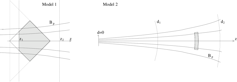
Fig. 1: Two geometries to account for the X-ray and TeV $\gamma$-ray emission from BL Lac objects. On the left side, the emitting particles fill a volume (shaded grey here) made up of two back-to-back cones. The geometry might result from a single larger cone (dotted line), where the number of electrons tapers off after some time. The right side shows a shell of high-energy particles traveling down the jet. Such a geometry might result from an electromagnetic shower developing close to the black hole. In both geometries, the emitting electrons and/or positrons drift along the magnetic field lines, and start emitting within the regions delimited by $z_{1}$ and $z_{2}$, and by $d_{1}$ and $d_{2}$, respectively. The true geometry might lie between the two extremes shown here.

In Model 1 the high-energy electrons fill a shape that resembles two back-to-back cones with a maximum cone radius of $R$ and a total length of $2\,R$ along the jet axis (Fig. 1, left side). The specific geometry chosen here reproduces the triangle shaped flares commonly observed in X-ray and TeV-$\gamma$-ray light curves of blazars. Note that the exact shape of the region is not very important. The important property of Model 1 is that the diameter divided by the speed of light equals approximately the observed flare duration. For simplicity we choose an identical height and length of the emitting volume. More realistic shapes may be obtained from modeling how an $e^{+}/e^{-}$ spark forms in a high electric field region. We assume that the leptons follow the magnetic field lines dissipating little energy until they enter the radiation zone at a distance $z_{1}$ from the black hole in which some instability causes the particles to move with an isotropic distribution of pitch angles $\theta$ to the magnetic field lines with $\theta<\theta_{\rm max}$. We assume that the electrons stop emitting when they exit the radiation zone at a distance $z_{2}$ from the black hole with $z_{2}-z_{1}\,=$ $2\,R$. The electrons may stop emitting because further instabilities slow them down. The duration $\Delta t_{\rm obs}$ of a flare is given by the length of the emission zone: $\Delta t_{\rm obs}\approx$ $(z_{2}-z_{1})\,/\,c\,=$ $2\,R\,/\,c$. For Mrk 501, typical flare durations are $\Delta t_{\rm obs}=$ 12 hrs and thus $R\,\approx$ 6.5 $(\Delta t_{\rm obs}/12{\rm~{}hrs})$ 10${}^{14}\,$cm. Each electron spends a time $\Delta t_{\rm rad}=$ $\Delta t_{\rm obs}$ in the emission region. Here and in the following model, the emitting particles travel together with the emitted photons down the jet with the main velocity dispersion originating from the pitch angle distribution of the leptons and photons.

Model 2 describes a spatial electron/positron distribution that might result from a synchrotron/pair-creation cascade of extremely high-energy particles accelerated by strong electric fields close to the black hole. We assume that the electrons move along magnetic field lines that make angles $\alpha$ up to $\alpha_{\rm max}$ to the jet axis and are concentrated in a spherical or conical shell or “shower front” that travels down the jet axis (Fig. 1, right side). We assume that the electrons only emit in a radiation zone that extends from a distance $d_{1}$ to $d_{2}$ from the black hole. Within the emission zone the electrons spiral with pitch angles $\theta<\theta_{\rm max}$ around magnetic field lines.

We assume $d_{1}\equiv d_{2}/2$ and consider only the case where the jet points exactly at the observer. High-Lorentz factor electrons emit synchrotron and inverse Compton emission only along the direction of their motion. Taking into account the electron pitch angle distribution, observers can only see the emission from electrons traveling along field lines with $\alpha\,\leq$ $\theta_{\rm max}$. Based on the standard equations from the description of superluminal motion (Blandford, McKee, & Rees, 1977) and neglecting $(\cos{(\theta_{\rm max})})$ factors, we get

$$\Delta t_{\rm obs}\,\approx\,\frac{\kappa\,d_{2}\,+\,T}{c}{\rm~{}~{},~{}with~{}~{}}$$ (1)

$$\kappa\,=\,1\,-\,\cos{\theta_{\rm max}}\,\approx\,\frac{1}{1642}\,\left(\frac{\theta_{\rm max}}{2^{\circ}}\right)^{2}$$ (2)

As the electrons travel from $d_{1}$ to $d_{2}$, their different pitch angles result in an increase of the thickness of the shell by $\Delta T\,\approx$ $\kappa\,(d_{2}-d_{1})$ . Taking into account that the shell has already a finite thickness at $d_{1}$, we use in simple approximation a constant shell thickness of

$$T\,=\,\kappa\,d_{2}$$ (3)

Combining eqs. (1) and (3), we get

$$d_{2}\,\approx\,\frac{c\,\Delta t_{\rm obs}}{2\,\kappa}\,\approx\,10^{18}~{}\left(\frac{\Delta t}{\rm 12~{}hrs}\right)\left(\frac{\theta_{\rm max}}{2^{\circ}}\right)^{-2}~{}\rm cm$$ (4)

The thickness is $T\,=$ $c\,\Delta t_{\rm obs}\,/2\,=$ 6.5$\cdot 10^{14}$ $(\Delta t_{\rm obs}/{\rm 12~{}hrs})$ cm. At $d_{2}$ the shell has the following height perpendicular to the jet axis

$$H\,=\,\frac{c\,\Delta t_{\rm obs}\,\sin{\theta_{\rm max}}}{2\kappa}\,\approx\,3.7\cdot 10^{16}~{}\left(\frac{\Delta t}{\rm 12~{}hrs}\right)\left(\frac{\theta_{\rm max}}{2^{\circ}}\right)^{-1}~{}\rm cm$$ (5)

For $d_{1}\,=$ $d_{2}/2$, each electron spends a time $\Delta t_{\rm rad}\,=$ $(d_{2}-d_{1})/c\,=$ $\Delta t_{\rm obs}\,/\,(4\,\kappa)$ in the emission region. In Model 2, triangle shaped pulses could result from a particle density that drops at a certain distance from the jet axis.

Models 1 and 2 represent extreme geometries. The true geometry may lie between these two extremes.

2.2 Simple Analytical Considerations

In this section, we use some simple analytical estimates to derive insights about the beam parameters and their scaling behavior with the model parameters. Further below, we will see that the inverse Compton emission is mainly emitted in the Klein-Nishina regime where the electrons give most of their energy to the scattered photons. The observation of $\sim$20 TeV photons thus implies the presence of electrons with Lorentz factors $\gamma_{0}\,=$ 4$\cdot 10^{7}$ and energy $E_{\rm e}\,=$ $\gamma_{0}m_{\rm e}c^{2}\,=$ 20 TeV. From the BeppoSAX X-ray observations on April 16, 1997 (Pian et al., 1998; Massaro et al., 2004) we infer an 0.1 keV-200 keV energy flux of $\hat{I}_{\rm x}\,=$ $4\cdot 10^{-9}$ ergs cm^-2 sec^-1. The observations did not cover the entire flare, and we assume here that the flux averaged over the flare duration was half the peak flux $I_{\rm x}\,=\hat{I}_{\rm x}/2$. If the source at distance $D$ emits into the solid angle $\Delta\Omega\,\approx$ $2\,\pi$ $(1-\cos{\sqrt{\alpha_{\rm max}\,\!^{2}+\theta_{\rm max}\,\!^{2}}})$, the time averaged X-ray luminosity during the flare is

$$L_{\rm x}\,=\,I_{\rm x}\,\Delta\Omega\,D^{2}\,\approx\,3\cdot 10^{42}\,{\rm~{}erg~{}sec}^{-1}$$ (6)

The total energy emitted into the X-ray band is

$$W_{\rm x}\,=\,\Delta t_{\rm obs}\,L_{\rm x}$$ (7)

Electrons with Lorentz factor $\gamma$ moving with pitch angles $0<\theta<\theta_{\rm max}\,\ll$ 1 emit synchrotron radiation at a mean critical frequency

$$\nu_{\rm c}\,=\,\frac{e\,\gamma^{2}\,B\,\theta_{\rm max}}{2\,\pi\,m_{\rm e}\,c}$$ (8)

For a Lorentz factor $\gamma_{0}$, the frequency of synchrotron emission equals $\nu_{\rm s0}\,\equiv$ 2.4$\cdot 10^{17}$ Hz for a magnetic field

$$B\,=\frac{2\,\pi\,m_{\rm e}\,c\,\nu_{\rm s0}}{e\,\gamma_{0}\,\!^{2}\,\theta_{\rm max}}\,\approx\,0.016~{}\left(\frac{\nu_{\rm s0}}{2.4\cdot 10^{17}\rm~{}Hz}\right)\left(\frac{\gamma_{\rm 0}}{4\cdot 10^{7}}\right)^{-2}\left(\frac{\theta_{\rm max}}{2^{\circ}}\right)^{-1}~{}\rm G$$ (9)

where $h$ is Planck’s constant. Averaged over pitch angles, the synchrotron power per electron is

$$p_{\rm s}\,=\,\frac{e^{4}\,\gamma_{0}\,\!^{2}\,B^{2}\,\theta_{\rm max}\,\!^{2}}{3\,m_{\rm e}\,\!^{2}\,c^{3}}\,\approx\,3.9\cdot 10^{-7}~{}\left(\frac{\nu_{\rm s0}}{2.4\cdot 10^{17}\rm~{}Hz}\right)^{2}\left(\frac{\gamma_{\rm 0}}{4\cdot 10^{7}}\right)^{-2}{\rm~{}erg~{}sec}^{-1}$$ (10)

The synchrotron cooling time $t_{\rm s}\,=$ $E_{\rm e}/p_{\rm s}$ is

$$t_{\rm s}\,=\frac{3\,m_{\rm e}\,\!^{3}\,c^{5}}{e^{4}\,\gamma_{\rm 0}\,B^{2}\,\theta_{\rm max}\,\!^{2}}\,\approx\,8.3\cdot 10^{7}\left(\frac{\nu_{\rm s0}}{2.4\cdot 10^{17}\rm~{}Hz}\right)^{-2}\left(\frac{\gamma_{\rm 0}}{4\cdot 10^{7}}\right)^{3}{\rm~{}sec}$$ (11)

In Model 1, the electrons spend a time $\Delta t_{\rm obs}$ in the emission zone and radiate only $\sim t_{\rm s}\,/$ $\Delta t_{\rm obs}\,$ $\approx 0.05$% of their energy before leaving it. Given that the total synchrotron and inverse Compton luminosities are approximately equal, we see that the emitting particles radiate away only 0.1% of their energy. Model 1 is thus radiatively very inefficient. The efficiency does not depend strongly on details of the shape of the emitting region, as long as the length of the emission region equals approximately the flare duration. The scaling with the model input parameters shows that the efficiency is independent of the electron pitch angle distribution. It is lower if electrons with energies exceeding 20 TeV emit the observed synchrotron emission.

In Model 2, the emission zone is more extended. For this model, a rough estimate shows that the combined synchrotron and inverse Compton cooling time $\left(t_{\rm s}\,\!^{-1}+t_{\rm ic}\,\!^{-1}\right)^{-1}$ equals approximately the time $\frac{1}{4\,\kappa}\,\Delta t_{\rm obs}$ that the emitting particles stay in the emission region. Model 2 is thus radiatively very efficient.

A total number of electrons

$$N_{\rm e}\,=\,\frac{W_{\rm x}}{\Delta t_{\rm rad}\,p_{\rm s}} = \frac{L_{\rm x}}{p_{\rm s}}\,\approx\,8.5\cdot 10^{48}~{}~{}{\rm(Model~{}1)}$$ (12)

$$= 4\,\kappa\,\frac{L_{\rm x}}{p_{\rm s}}\,\approx\,2\cdot 10^{46}~{}~{}{\rm(Model~{}2)}$$ (13)

produce the flare. The models require a particle luminosity averaged over the duration of the flare of

$$L_{\rm e}\,=\,\frac{N_{\rm e}\,\gamma_{\rm 0}\,m_{\rm e}\,c^{2}}{\Delta t_{\rm rad}} \approx 6.3\cdot 10^{45}~{}{\rm erg~{}sec}^{-1}~{}~{}{\rm(Model~{}1)}$$ (14)

$$\approx 1.5\cdot 10^{43}~{}{\rm erg~{}sec}^{-1}~{}~{}{\rm(Model~{}2)}$$ (15)

For Model 2 it is indeed the observed flare duration and not the time $\Delta t_{\rm rad}$ that is relevant for computing the power required for sustaining continued flaring activity. These luminosities are minimum luminosities to produce the observed X-ray emission. There may be additional electrons that produce X-ray emission outside the BeppoSAX energy band.

The electron beam of Model 2 resembles in some aspects the blobs filled with emitting particles of the reference model. This is not too surprising as both models assume that the radiation is emitted as synchrotron-Compton emission. The different models result in some differences in the phase space distribution of the electrons and photons. Furthermore, the beams in Models 1 and 2 could be made entirely of high-energy particles. The reference model assumes the presence of a support medium of rather cold particles, and shocks are invoked to explain how the energy of the bulk of cold particles is transferred to a few high-energy particles.

It is instructive to compare these jet luminosities to the Eddington luminosity. Based on bulge stellar dispersion measurements, the best estimate of the black hole mass in Mrk 501 is $M_{\rm BH}\,\approx$ $10^{9}$ $M_{\odot}$ (Falomo, Kotilainen & Treves, 2002; Barth, Ho, & Sargent, 2003). The Schwarzschild radius thus is

$$r_{\rm Sch}\,=\,2\,G\,M_{\rm BH}\,/\,c^{2}\,=\,3\cdot 10^{14}\,\frac{M_{\rm BH}}{10^{9}M_{\odot}}{\rm~{}cm}$$ (16)

and the expression for the Eddington luminosity reads

$$L_{\rm Edd}\,=\,\frac{4\,\pi\,c\,m_{\rm p}\,G\,M_{\rm BH}}{\sigma_{\rm T}}\,=\,1.25\cdot 10^{47}~{}\frac{M_{\rm BH}}{10^{9}M_{\odot}}~{}{\rm erg~{}sec}^{-1}$$ (17)

It is roughly 20 and 10⁴ higher than the minimum luminosities required by Models 1 and 2, respectively.

2.3 Numerical Results

While the analytic estimates allow us to understand the scaling of the power-requirements, they are not appropriate for describing the inverse Compton component and internal $\gamma$-ray absorption processes as these two depend on the details of the synchrotron photon energy spectrum. The following numerical estimates use electron energy spectra $dN_{\rm e}/d\gamma$ instead of a mono-energetic electron distribution. We use energy spectra that resemble broken power laws over small dynamic ranges with a ratio of the maximum to minimum Lorentz factor of $\sim 100$. The synchrotron power emitted by the leptons at frequency $\nu$ per frequency interval d$\nu$ is computed using the standard equation (Rybicki & Lightman, 1979):

$$P_{\rm s}(\nu)\,=\,c_{1}\,\int_{\gamma_{\rm min}}^{\gamma_{\rm max}}d\gamma~{}\int_{0}^{\theta_{\rm max}}\sin\theta~{}d\theta~{}\frac{dN_{\rm e}}{d\gamma}~{}\frac{3\,e^{3}\,B\,\sin{\theta}}{m_{\rm e}\,c^{2}}~{}F(x)$$ (18)

where the first integral runs over the electron Lorentz factors and the second averages over the pitch angle distribution. Here and in the following we use the constant $c_{1}\,\equiv$ $(1-\cos{\theta_{\rm max}})^{-1}$ to normalize the integrals over the pitch angle distribution. The function $F(x)$ equals $x\int_{x}^{\infty}~{}K\frac{5}{2}(\xi)~{}d\xi$ with $K\frac{5}{2}$ the modified Bessel function of $5/2$ order, and $x\,=$ $\nu\,/\,\nu_{\rm c}$. The emitted inverse Compton power is approximately given by

$$P_{\rm ic}(\nu)\,=\,c_{1}\,\int_{\gamma_{\rm min}}^{\gamma_{\rm max}}d\gamma~{}\int_{\nu_{\rm min}}^{\nu_{\rm max}}d\nu_{\rm s}~{}\int_{0}^{\theta^{\prime}_{\rm max}}\sin\theta~{}d\theta~{}\frac{dN_{\rm e}}{d\gamma}~{}\,c\left(1-\cos{\theta}\right)\,\sigma_{\rm KN}(y)\,n_{\rm s}(\nu_{\rm s})\,\Delta E(y)$$ (19)

Here we use $\theta^{\prime}_{\rm max}\,=\,\theta_{\rm max}$ in rough approximation. The last term in the integrand is the energy that a photon gains in a scattering. The other terms give the scattering rate that depends on the angle between the electron and photon velocity vectors and on the density of synchrotron photons $n_{\rm s}$. The Klein-Nishina cross section is to good approximation

$$\sigma_{\rm KN}(y)\,=\,\frac{3}{8}\,\frac{\ln{(2\,y)}+0.5}{y}\,\sigma_{\rm T}$$ (20)

where $\sigma_{\rm T}$ is the Thomson cross section. The value $y$ is the photon energy in the electron rest frame in units of the electron rest mass

$$y\,=\,\frac{h\,\nu_{\rm s}\,\gamma_{\rm 0}\,(1-cos{\theta})}{m_{\rm e}\,c^{2}}$$ (21)

Following Dermer & Schlickeiser (1993), we use the approximation

$$\Delta E(y) = y\,\gamma\,m_{\rm e}\,c^{2}{\rm~{}for~{}}y~{}<~{}1{\rm~{}and~{}}$$ (22)

$$= \gamma\,m_{\rm e}\,c^{2}\hskip 7.68236pt{\rm~{}for~{}}y~{}\geq~{}1$$ (23)

For Model 1, $n_{\rm s}$ can be computed as follows. The total number of photons emitted in a certain frequency interval over the duration of the flare is $N_{\rm s}(\nu)\,=$ $\Delta t_{\rm obs}\,P_{\rm s}(\nu)\,/$ ${h\,\nu}$. The emitting particles occupy a volume of $\pi\,R^{3}$. Taking into account that the photon density rises from 0 to its final value as the emitting particles move through the emission region, the time averaged photon density is

$$n_{\rm s}(\nu)\,=\,\frac{1}{2\,\pi\,R^{3}}\,\frac{\Delta t_{\rm obs}\,P_{\rm s}(\nu)}{h\,\nu}~{}~{}{\rm(Model~{}1)}$$ (24)

In the case of Model 2, a similar argument gives after some arithmetic:

$$n_{\rm s}(\nu) = \frac{2\,(1-\ln{2})}{\pi\,(\Delta t_{\rm obs}\,c)^{3}}\,\frac{\Delta t_{\rm obs}\,P_{\rm s}(\nu)}{h\,\nu}~{}~{}{\rm(Model~{}2)}$$ (25)

The factor $(1-\ln{2})$ arises from averaging the synchrotron photon density over the time the emitting particles travel from $d_{1}$ to $d_{2}$, taking into account that the shell height increases from $H/2$ to $H$ and the number of synchrotron photons increases linearly from 0 to its final value. Finally, the time averaged fluxes received at Earth can be computed from:

$$I(\nu) = \frac{P_{\rm s}(\nu)+P_{\rm ic}(\nu)}{\Delta\Omega\,D^{2}}~{}~{}{\rm(Model~{}1)}$$ (26)

$$= \frac{\Delta t_{\rm rad}\,(P_{\rm s}(\nu)+P_{\rm ic}(\nu))}{\Delta t_{\rm obs}\,\Delta\Omega\,D^{2}}\,=\,\frac{P_{\rm s}(\nu)+P_{\rm ic}(\nu)}{4\,\kappa\,\Delta\Omega\,D^{2}}~{}~{}{\rm(Model~{}2)}$$ (27)

The optical depth per path length for $\gamma\gamma\,\rightarrow$ $e^{+}\,e^{-}$ processes is computed with the equations of Gould & Schréder (1967)

$$\frac{d\tau_{\rm int}}{dz}(\nu_{\gamma})\,=\,c_{1}\,\int_{0}^{\theta_{\rm max}}\sin{\theta}d\theta~{}\int_{\nu_{\rm thr}}^{\infty}d\nu~{}\sigma_{\gamma\gamma}\,n_{\rm s}(\nu)\,(1-\cos{\theta})$$ (28)

The first integral runs over the pitch angle distribution and the second integrates over the target photon frequencies. The threshold frequency for pair creation reads

$$\nu_{\rm thr}\,=\,\frac{2\,(m_{\rm e}\,c^{2})^{2}}{h^{2}\,\nu_{\gamma}\,(1-\cos{\theta})}$$ (29)

and the pair-creation cross section is

$$\sigma_{\gamma\gamma}\,=\,\frac{3\,\sigma_{\rm T}}{16}(1-\beta^{2})\left[2\,\beta\,(\beta^{2}-2)+(3-\beta^{4})\,ln{\left(\frac{1+\beta}{1-\beta}\right)}\right]~{}{\rm cm}^{2}$$ (30)

with $\beta\,=$ $\sqrt{1-\nu_{\rm thr}/\nu}$. In the following, we focus only on absorption by synchrotron photons. Absorption by external (e.g. disk) photons will briefly be discussed in Sect. 3.2. For Model 1, the optical depth is approximately $R\,d\tau_{\rm int}/dz$ and for Model 2 it is $\frac{1}{2}(d_{2}-d_{1})\,d\tau_{\rm int}/dz$.

The optical depth for extragalactic pair-creation processes is computed based on the model of the extragalactic background light (EBL) from Kneiske, Mannheim, & Hartmann (2002) and Kneiske, Bretz, Mannheim, & Hartmann (2004). This model is almost identical to the model P045 of Aharonian et al. (2006) and is thus consistent with the observed energy spectra of two distant BL Lac objects detected with the H.E.S.S. experiment. An equation similar to eq. (30) is used with the modifications that the integral over pitch angles goes from 0 to $\pi$ and the EBL target photon density is used.

The models together with the BeppoSAX and CAT energy spectra are shown in Fig. 2. We use the BeppoSAX data reanalyzed by G. Fossati (private communication, 2006) and the CAT data from (Djannati-Atai et al., 1999). In the case of the CAT data, we show the systematic (rather than statistical) errors which seem to be the dominant ones. Comparing TeV $\gamma$-ray energy spectra taken with different Cerenkov telescope experiments (including CAT) we obtain a one sigma systematic error on TeV spectral indices of approximately 0.2.

The difference of the solid and dotted lines in Fig. 2 shows the effect of extragalactic $\gamma$-ray absorption. Although the emitted inverse Compton components peak at and above $>$5 TeV, the absorbed energy spectra are rather soft compared to the measured SEDs. Models with harder $\gamma$-ray energy spectra can be produced with inverse Compton processes deeper in the Klein-Nishina regime. We did not implement this possibility here as the resulting models do not fully account for the $<1$ keV BeppoSAX data, and would thus require additional X-ray emission from downstream plasma to reproduce the $<1$ keV flux.

The specific choices of model parameters result in mechanical luminosities of 2.3$\cdot 10^{46}$ erg sec^-1 and 2.7$\cdot 10^{44}$ erg sec^-1 for Model 1 and 2, respectively. For Model 1, we fitted the data using $\Delta t_{\rm obs}\,=$ 22 hrs, $\theta_{\rm max}\,=$ $1^{\circ}$, $\alpha_{\rm max}\,=$ $1^{\circ}$ as the main input parameters. For Model 2, we used $\Delta t_{\rm obs}\,=$ 12 hrs, $\theta_{\rm max}\,=$ $2^{\circ}$, and $\alpha_{\rm max}\,=$ $3^{\circ}$. Compared to the parameters of Model 1, we had to assume for Model 2 a larger solid angle into which the radiation is emitted and a shorter $\Delta t_{\rm obs}$ in order to reproduce the TeV $\gamma$-ray flux level. The power requirement for Model 2 could be reduced to a value close to the one in eq. (15) with smaller $\theta_{\rm max}$ and $\alpha_{\rm max}$ values and assuming the presence of external seed photons, for example from an outer slower layer of the jet similar as in the model of Ghisellini, Tavecchio, & Chiaberge (2005).

The main conclusions from the more detailed modeling are that (i) parallel beam synchrotron self-Compton models are viable without requiring external seed photons to account for the observed $\gamma$-ray emission, (ii) internal absorption effects are small or negligible, and (iii) that the high-energy beams require so much power that power efficient beam formation models are strongly preferred.

3 Origin of the parallel electron beam

3.1 Constraints from the Total Energetics

We concentrate here on electromagnetic models as they predict powerful large-scale magnetic and electric fields that might be able to accelerate particles to very high energies and produce large-scale ordered motion. Three geometries for accelerating particles in electromagnetic models have been discussed in the literature. The models assume that the black hole and accretion disk are embedded in a conducting magnetosphere. Free charge carriers are created in the magnetosphere through cascades involving curvature radiation or inverse Compton scattering and pair creation processes. A quasi-stationary configuration is achieved if the charge carriers are distributed such that $\vec{E}\cdot\vec{B}\,=0$. If this condition is fulfilled, charged particles move along magnetic field lines without gaining or loosing energy. The magnetosphere can act as a series of nearly parallel conductors with zero resistance along the magnetic field lines that can sustain a voltage drop far away from where it was generated. The voltage drop may either be generated by the disk itself (Lovelace, 1976; Blandford, 1976), or by the Kerr black hole spinning in the horizon-threading magnetic field supported by the disk (Blandford & Znajek, 1977; Thorne et al., 1986). Katz (2006) argues that the electric field generated by a homopolar generator in a rotating magnetized fluid has curls in the observers frame and cannot be shorted out at all locations by a stationary charge distribution. It thus seems likely that non-stationary vacuum gaps form, which are capable of accelerating particles. A possible geometry of the magnetosphere and the gap region is shown in Figure 3. The formation of the gap close to the rotation axis might explain the initial collimation of the jet.

In electromagnetic models, the Poynting flux launches the jet and anchors the jet to the disk or black hole. For simplicity we focus here on disk models; some considerations are applicable to the Blandford-Znajek model as well. We assume that the coordinate system $r$, $\phi$, $z$ is aligned with the jet and the black hole resides at its origin. Directly above the disk, the Poynting flux is

$$\vec{S}\,=\,\frac{c}{4\,\pi}\,\vec{E}\times\vec{B}\,=\,\frac{c}{4\,\pi}\,\vec{E}_{\rm p}\times\vec{B}_{\rm t}$$ (31)

where the subscripts p and t denote the poloidal ($r$ and $z$) and toroidal ($\phi$) components, respectively. The second equality follows from the fact that the toroidal electric field vanishes for a stationary axisymmetric solution. The condition that the electric field $\vec{E}^{\prime}$ in the frame co-rotating with the disk material vanishes gives

$$0\,=\,\vec{E^{\prime}}\,=\,\vec{E}_{\rm p}\,+\frac{1}{c}\left(\vec{\Omega}\times\vec{r}\right)\times\vec{B}_{\rm p}$$ (32)

with $\vec{\Omega}\,=$ (0,0,$\Omega$) the angular velocity of the disk material at location $\vec{r}$. Thus, the poloidal electric field satisfies

$$\vec{E}_{\rm p}\,=\,-\frac{1}{c}\,\left(\vec{\Omega}\times\vec{r}\right)\times\vec{B}_{\rm p}$$ (33)

Combining eqs. (31) and (33), the magnitude of the Poynting flux is

$$S\,=\,\frac{1}{4\pi}\,\Omega\,r\,B_{\rm p}\,B_{\rm t}$$ (34)

If we now use

$$\Omega\,r\,=\,\left(\frac{G\,M_{\rm BH}}{r}\right)^{1/2}$$ (35)

and assume

$$B_{\rm t}(r) = B_{\rm t,r_{1}}\,(r/r_{1})^{-1}$$ (36)

$$B_{\rm p}(r) = B_{\rm p,r_{1}}\,(r/r_{1})^{-1}$$ (37)

the power transported by the Poynting flux perpendicular to the disk surface is

$$L_{\rm disk}\,=\,2\,\pi\,\int_{r_{1}}^{r_{2}}\,S\,r\,dr\,=\,\frac{6^{3/2}}{4\,c^{3}}\,\left(G\,M_{\rm BH}\right)^{2}\,B_{\rm t}\,B_{\rm p}\,\approx\,5\cdot 10^{44}\,\frac{M_{\rm BH}}{10^{9}\,M_{\odot}}\,\frac{B_{\rm t,r_{1}}}{10^{3}\,\rm G}\,\frac{B_{\rm p,r_{1}}}{200\,\rm G}{\rm~{}erg~{}sec}^{-1}$$ (38)

where we used $r_{1}\,\approx\,3\,R_{\rm Sch}$ and $r_{2}\,\gg\,r_{1}$. Thus, magnetic fields between $10^{2}$ and $10^{3}$ G are needed to form the beam of Model 2. Here and in the following, we use the rather high power requirement from the numerical SSC calculations. The reader should keep in mind that external Compton models would require $\sim$20 times less power. For Model 1, $B_{\rm t}$ and $B_{\rm p}$ have to be both roughly ten times higher. Various estimates of the magnetic field in accretion disks have been discussed by Ghosh & Abramowicz (1997). Magnetic fields of $\simeq 10^{4}$ G seem likely from dimensional arguments and numerical simulations.

The voltage drop across the disk from $r_{1}$ to $r_{2}\,\gg\,r_{1}$ is

$$V_{\rm 12}\,=\,\int_{r_{1}}^{r_{2}}\frac{1}{c}\,r\,\Omega\,B_{\rm p}\,dr\,=\,\frac{\sqrt{24}\,G\,M_{\rm BH}\,B_{\rm p,r_{1}}}{c^{2}}\,\approx\,4.3\cdot 10^{19}\,\frac{M_{\rm BH}}{10^{9}\,M_{\odot}}\,\frac{B_{\rm p,r_{1}}}{200\,\rm G}{\rm~{}V}$$ (39)

If $r_{2}\,=$ 2$\,r_{1}$ (rather than $r_{2}\gg r_{1}$), $L_{\rm disk}$ and $V_{\rm 12}$ are smaller by a factor of $(1-1/\sqrt{2})$. A natural mechanism for explaining the variable nature of the X-ray and TeV gamma-ray emission from blazars is screening of the voltage $V_{12}$ by electron/positron pairs. The Blandford-Znajek mechanism results in a qualitatively similar relations between the magnetic field, the electric fields, and the emitted power. The main difference is that the EMF is generated close to the event horizon rather than at the inner region of the accretion disk.

Given a poloidal magnetic field with $B_{\rm p,r_{1}}\,\approx$ 200 G at the base of the jet, we can estimate the magnetic field at the distance $d_{2}$ in the simple case that the poloidal magnetic field scales inversely proportional to the radius of the emission zone squared. For Model 2 we obtain

$$B_{\rm d1}\,=\,B_{\rm r_{1}}\,\left(\frac{r_{1}}{H}\right)^{2}\,=\,0.013~{}\left(\frac{B_{r_{1}}}{\rm 200~{}G}\right)~{}\left(\frac{H}{3.7\cdot 10^{16}\rm~{}cm}\right)^{-2}{\rm~{}G}$$ (40)

where $H$ is the radius of the emission zone perpendicular to the jet axis. This simple estimate agrees well with the value inferred from modeling the data (see eq. (9)).

3.2 Beam Formation

The number of electrons required to explain the X-ray and TeV $\gamma$-ray emission is so large that charge neutrality of the beam is important as otherwise the jet would expand too rapidly in the direction perpendicular to the jet axis. The maximum energy to which particles are accelerated depend on the relative magnitude of the energy gain and energy loss rates. The energy gain rate depends on $V_{12}$ and the distance over which the voltage drop occurs. Energy loss mechanisms are curvature radiation, synchrotron emission and inverse Compton emission. With curvature radii on the order of $r_{1}$, curvature losses are only important at very high $\gg$TeV energies. The magnitudes of the synchrotron and inverse Compton losses are highly uncertain as they depend on the magnetic field strength and particle pitch angle distribution, and on the intensity of the ambient photon field in the acceleration region, respectively. Synchrotron losses are negligible if electrons drift along magnetic field lines. Assuming scattering in the Thomson regime, a 20 TeV electrons loses the energy

$$\Delta E_{\rm ic}\,=\,\gamma_{0}\,\!^{2}\,(1-\cos{\vartheta})^{2}\,l_{\rm acc}\,\sigma_{\rm T}\,u_{\rm a}$$ (41)

when traveling a distance $l_{\rm acc}$ through an ambient photon field with energy density $u_{\rm a}$. Here, $\vartheta$ is the angle between the electron and photon velocity vectors. The energy losses are negligible when $u_{\rm a}$ satisfies

$$u_{\rm a} \ll \frac{m_{\rm e}\,c^{2}}{\gamma_{0}\,(1-\cos{\vartheta})^{2}\,l_{\rm acc}\,\sigma_{\rm T}}\,\approx\,0.002{\rm~{}erg~{}cm}^{-3}$$ (42)

for $\vartheta\,=$ 30^∘ and $l_{\rm acc}\,=\,r_{1}$. The ambient photon energy density corresponds to a luminosity of

$$L_{\rm a}\,=\,4\pi\,(30\,r_{1})^{2}\,c\,u_{\rm a}\,\approx\,5\cdot 10^{41}{\rm erg~{}sec}^{-1}$$ (43)

if the particle acceleration region is at a distance $30\,r_{1}$ from the photon source, presumably the accretion disk. Comparing the minimum beam luminosity required for producing the observed X-ray and TeV $\gamma$-ray emission (eq. (15)) with $L_{\rm a}$, we see that the model requires an accretion flow with a radiative efficiency of 3% or less. Higher disk luminosities are possible if the emission frequency is sufficiently high that the high-energy electrons interact only in the Klein-Nishina regime.

Lovelace (1976) assumed that protons may be accelerated all the way to ultra high energies and that quasars thus may be accelerators of ultra high energy cosmic rays (see Boldt & Ghosh 1999; Boldt & Loewenstein 2000; Levinson 2000 for similar recent papers). He stipulated that the flow of high-energy protons may entrain or pick up electrons. Assuming that the high-energy electrons and protons would move with identical velocities and Lorentz factors, the acceleration of protons would increase the minimum beam luminosity by the proton to electron mass ratio. For Model 1, the required luminosity would exceed the Eddington luminosity by at least two orders of magnitude. For Model 2, accretion with a few times the Eddington rate would be sufficient. With $B_{\rm p,r_{1}}\approx$0.17 G, eq. (39) predicts proton energies of $\approx 3\cdot 10^{16}$ eV and just the right electron energy of $\approx$20 TeV. However, a prohibitively strong toroidal magnetic field exceeding $10^{6}$ G would be required so that the Poynting flux can power the massive electron-proton beam.

The acceleration of electrons or positrons with subsequent entrainment of oppositely charged leptons would result in a beam with a much lower power. However, eq. (39) predicts an adequate voltage drop for a very weak poloidal magnetic field with $B_{\rm p,r_{1}}\,\approx$ $2\cdot 10^{-4}$ G. Even for Model 2, the beam power requires again a toroidal magnetic field exceeding $10^{6}$ G. Stronger $B_{\rm p,r_{1}}$ and weaker $B_{\rm t,r_{1}}$ would be viable if the leptons are accelerated to energies exceeding 40 TeV, and then entrain both electrons and positrons, slowing them down to a mean energy of $\sim$20 TeV per lepton.

Acceleration of electrons or positrons with $B_{\rm t}\sim B_{\rm p}$ would produce a few particles with very high energies. A natural way of transferring the energy from a few high-energy particles to many low-energy particles are cascades. Electromagnetic cascades in AGN jets have been discussed by (Burns & Lovelace, 1982; Blandford & Levinson, 1995; Levinson & Blandford, 1995). A generic discussion of electromagnetic cascades in the $>$TeV regime has been given in (Svensson, 1987). Unfortunately, cascade models need considerable fine tuning to produce the electron beams with the right properties. We briefly go through a specific scenario to emphasize some of the relevant difficulties. Electrons are accelerated until the energy gains in the electric field $E_{12}\,=V_{12}/l_{\rm acc}$ along magnetic field lines equal the energy losses. If curvature losses dominate, the energy loss rate reads

$$p_{\rm c}\,=\,\frac{2}{3}\,\frac{e^{2}\,c\,\gamma^{4}}{\rho^{2}}$$ (44)

with $\rho$ an average curvature radius, which gives a maximum Lorentz factor of

$$\gamma_{\rm max}\,=\,\left(\frac{3}{2}\,\frac{(V_{12}/l_{\rm acc})\,\rho^{2}}{e}\right)^{1/4}\,\approx\,10^{11}\left(\frac{V_{\rm 12}}{10^{19}\rm~{}V}\right)^{1/4}\,\left(\frac{l_{\rm acc}}{0.15\,r_{1}}\right)^{-1/4}\,\left(\frac{\rho}{r_{1}}\right)^{1/2}$$ (45)

which corresponds to an energy of 50 PeV. The highest-energy electrons emit curvature photons at frequency

$$\nu_{\rm c}\,=\,\frac{3}{4\pi}\,\frac{\gamma_{\rm max}\,\!^{3}\,c}{\rho}\,\approx 10^{28}\left(\frac{V_{\rm 12}}{10^{19}\rm~{}V}\right)^{3/4}\,\left(\frac{l_{\rm acc}}{0.15\,r_{1}}\right)^{-3/4}\,\left(\frac{\rho}{r_{1}}\right)^{-1/2}{\rm Hz}$$ (46)

corresponding to a photon energy of $\simeq$40 TeV. Overall, each lepton drifting through the acceleration region emits $\gamma$-rays with a total energy of $e\,V_{12}-\gamma_{\rm max}\,m_{\rm e}\,c^{2}$, while it escapes with a relatively small amount of kinetic energy $\sim\gamma_{\rm max}\,m_{\rm e}\,c^{2}$. A part of the energy in the $\gamma$-ray beam may be converted back to the leptonic sector if the optical depth for pair creation is approximately unity. The pair creation cross section (eq. (30)) reaches its maximum value of $\approx 1/4\,\sigma_{\rm T}$ for target photons of frequency $\nu_{\rm a}\approx 2\,\nu_{\rm thr}$. Assuming that the target photons have the frequency $\nu\,\approx$ $2\nu_{\rm thr}$, and that the curvature $\gamma$-rays are emitted at a distance $30\,r_{1}$ from the target photon source, we infer a minimum target photon luminosity of 1.4$\cdot 10^{41}$ erg sec^-1 for which the pair creation optical depth for 40 TeV $\gamma$-rays escaping to infinity equals unity. The model requires fine-tuning as seed photons of frequency $\approx 2\,\nu_{\rm thr}$ are needed to suppress inverse Compton processes of $>$20 TeV electrons. If the target photon field is sufficiently intense, a cascade with several generations of photons and pairs can be initiated. The end-product of the cascade then depends on the energy spectrum and spatial gradient of the target photons.

Proton induced synchrotron/pair-creation cascades (PIC) in blazars have been discussed by (Mannheim, 1993; Mücke & Protheroe, 2001; Mücke et al., 2003). These models produce $\gamma$-rays as synchrotron emission of high-energy electrons/positrons with possible contributions from other secondary cascade particles. The models require not only high-energy protons, but also co-spatially accelerated electrons. The latter emit the radiation field that causes the protons to photo-produce mesons, and explain the observed X-ray emission. PIC models had originally been proposed in the framework of the shock-acceleration picture. A re-evaluation of these models with regards to accelerating the protons and electrons in the strong electric fields in the surrounding of a black hole may be a worthwhile enterprise, but is outside of the scope of this paper.

4 Discussion

This paper discusses the possibility that the X-ray and TeV $\gamma$-ray radiation from BL Lac type objects is emitted by parallel electron-positron beams that are accelerated by strong electric fields close to the accreting central black hole. For the first time we attempt to explain both the X-ray and TeV $\gamma$-ray emission from these objects with such a model. Fitting the model to data from the BL Lac object Mrk 501, we find that the particle acceleration zone and the X-ray and TeV $\gamma$-ray emission zone have to be spatially distinct. Otherwise, the large magnetic fields required to launch the jets prohibit the simultaneous emission of the X-rays and TeV $\gamma$-rays as synchrotron and inverse Compton radiation, respectively. Previous papers discussing the high-energy emission from blazars dismissed the possibility that the high-energy particles producing the observed radiation may be accelerated close to the black hole. It was believed that the co-spatially emitted radio to optical emission would cause an inverse Compton catastrophe, causing the high-energy particles to lose all their energy. For several reasons this argument is not valid for all blazars. First, in contrast to the situation in powerful quasars, the accretion disks of BL Lac objects are not radiating efficiently. For most BL Lac objects, there are only upper limits on the disk luminosity. Furthermore, a common assumption had been that the observed radio to optical radiation from BL Lac objects was emitted co-spatially with the X-ray and TeV $\gamma$-ray emission. For some objects like Mrk 501, this assumption had to be dropped even for the reference model, as the upper limits on the size of the emission region from the observed flux variability time scales resulted in synchrotron self-absorption cut-offs in the 100-1000 GHz range. Thus, even the standard model requires that at least the radio emission is produced further downstream in the jet than the X-ray and TeV $\gamma$-ray emission. In BL Lac objects, the observation campaigns carried through so far have not produced solid evidence for a correlation between the X-ray/TeV gamma-ray fluxes and the infrared-optical fluxes. Thus, also the infrared and optical emission may be produced downstream of the X-ray and TeV $\gamma$-ray emission, or even by independent processes. Two other factors contribute to the suppression of an inverse Compton catastrophe. In the parallel beam model the emitting particles and the photons travel almost in parallel, greatly reducing their interaction rate; furthermore, inverse Compton interactions of $>$TeV electrons and positrons with all photons with wavelengths shorter than a few microns are Klein-Nishina suppressed.

In the reference model, the jet is launched electromagnetically and the jet power is subsequently transferred to particles which carry it to large distances from the accretion system. Shocks in the jet medium transfer the energy transported by a large number of cold particles to high-energy particles that emit the observed radiation. Compared to this reference model, the model discussed here avoids the need for transferring the power first from Poynting flux to a large number of particles and then to transfer it back to a few high-energy particles. Furthermore, the parallel electron-positron beam model can cope with some of the difficulties of the reference model:

1. The model can explain the “odd” energy spectra of emitting electrons/positrons inferred from synchrotron-Compton fits to BL Lac data with more ease than the Fermi acceleration mechanisms. The most striking features are particle distribution functions almost resembling “delta-functions” or Maxwellian distributions. Such particle distribution might result from the acceleration and/or cascading processes discussed above.

2. The parallel beam model accounts for the non-detection of one of the tell-tale signatures of Fermi-type acceleration mechanisms, namely a particularly soft energy spectrum during the early rising phases of flares.

3. A consequence of the nearly parallel flow of the emitting particles and photons in the emission region are nearly simultaneous variations of the synchrotron and inverse Compton fluxes if fluxes emitted by electrons of similar energies are sampled, and if complications arising from cooling of electrons and thus an increase in seed photons can be neglected. Synchrotron self-Compton models in which the emitting particles move isotropically in the jet frame, predict that the synchrotron fluxes should rise faster than the inverse Compton fluxes (Coppi & Aharonian, 1999). Although such a time lag has long been searched for, it has eluded detection so far.

4. Sources like Mrk 501 and Mrk 421 show extended flaring periods with many flares. Furthermore, observations of Mrk 501 in 1997 showed an astonishing stability of the TeV $\gamma$-ray energy spectrum during the entire observation campaign (Krawczynski, et al., 2000). The X-ray and TeV $\gamma$-ray fluxes followed the same correlation during many distinct flares over a time period of several months. In the parallel beam model, regular and rather uniform flaring might result from alternating between shorting out and evacuating the particle acceleration region. Particle-accelerating recollimation shocks at certain typical distances from the central engines provide a viable alternative explanation. In contrast, models in which flares are produced by collisions of plasma blobs have difficulties to do so (Tanihata et al., 2003).

5. In the reference model, the high-energy particles move isotropically. As the particle pressure dominates over the magnetic field pressure by many orders of magnitude (Kino, Takahara, & Kusunose, 2002; Krawczynski et al., 2002), the model has difficulties to explain why the particles do not flow out of the emission volume with the speed of light. In the parallel beam model, the motion of the emitting particles along ordered magnetic field lines explains the beam collimation more naturally.

The parallel beam model has its own challenges. The discussion in the previous section indicates that direct particle acceleration followed by entrainment of ambient matter and the study of electromagnetic cascades in the TeV-PeV energy regime are areas where more detailed modeling is required. Another area for future work is more detailed time resolved simulations of the temporal evolution of the beam.

In the introduction we mentioned the discrepancy between jet bulk Lorentz factors inferred from the reference model to the X-ray and TeV $\gamma$-ray data, and from VLBA observations. Both, the reference model, and the parallel beam model can solve this problem by positing that the emission of the X-rays and TeV $\gamma$-rays is the start of a drastic energy dissipation of the jet. Model 2 is radiatively very efficient so that a considerable fraction of the jet energy goes directly into radiation. If radiatively inefficient models apply, the jet may slow down by entraining ambient material.

In the reference model, the difference between the emission of quasars and BL Lac objects is commonly attributed to a difference of the maximum energy of accelerated particles owing to more efficient inverse Compton cooling of accelerated particles in the intense radiation fields of quasars (Ghisellini et al., 1998). The parallel beam model has the potential to explain not only that the SEDs of quasars and BL Lac objects are different, but also that the kpc-scale jets are different. In the reference model, the intense photon fields only affect the particles accelerated by the jet far away from the central engine. In the parallel beam model, they can affect the process of jet formation itself. Thus, the intense radiation fields of quasars may prevent a parallel particle beam from forming altogether, and may allow a different jet formation mechanism to produce the powerful quasar jets.

Fig. 2: Results from modeling the Mrk 501 data from April 16, 1997 with the parallel beam model. The left and right panels show fits with Model 1 and Model 2, respectively. The solid and dotted lines show the emission with and without accounting for extragalactic absorption in $\gamma\gamma\rightarrow e^{+}e^{-}$ pair creation processes. The April 16 flare was the brightest of a large number of flares detected during a 6 month period. We show here the BeppoSAX X-ray and CAT $\gamma$-ray fluxes at only 50% of their measured values, to take into account that the observations did not cover the entire flare and that the fluxes averaged over the entire duration of the flare are likely to be lower than those measured at the peak of the flare. In the case of the CAT spectrum the shaded area shows the systematic uncertainties which dominate over the statistical uncertainties. The model parameters are given in the text.

Fig. 3: Snapshot of the magnetosphere and a non-stationary vacuum gap above an accreting black-hole system. Close to the black hole and the disk, the magnetosphere is filled with low-energy $e^{+}/e^{-}$ pairs that move along electric equipotential surfaces (dashed lines). Further away, there is a vacuum gap with a voltage drop $V_{12}\,=$ $V_{2}-V_{1}$ that can accelerate particles to $>$TeV energies. See Lovelace, MacAuslan, & Burns (1979) and Lovelace & Ruchti (1983) for a slightly different geometry.

References

- Aharonian (2000) Aharonian, F. A. 2000, New A, 5, 377
- Aharonian et al. (2006) Aharonian, F., et al. 2006, Nature, 440, 1018
- Aharonian et al. (2005) Aharonian, F., et al. 2005, A&A, 441, 465
- Aharonian et al. (1999) Aharonian, F. A., et al. 1999, A&A, 342, 69
- Barth, Ho, & Sargent (2003) Barth, A. J., Ho, L. C., & Sargent, W. L. W. 2003, ApJ, 583, 134
- Begelman, Blandford, & Rees (1984) Begelman, M. C., Blandford, R. D., & Rees, M. J. 1984, Reviews of Modern Physics, 56, 255
- Blandford (1976) Blandford, R. D. 1976, MNRAS, 176, 465
- Blandford & Levinson (1995) Blandford, R. D., & Levinson, A. 1995, ApJ, 441, 79
- Blandford, McKee, & Rees (1977) Blandford, R. D., McKee, C. F., & Rees, M. J. 1977, Nature, 267, 211
- Blandford & Payne (1982) Blandford, R. D., & Payne, D. G. 1982, MNRAS, 199, 883
- Blandford & Rees (1978) Blandford, R. D., & Rees, M. J. 1978, Pittsburgh Conference on BL Lac Objects, Pittsburgh, Pa., April 24-26, 1978, Proceedings. (A79-30026 11-90) Pittsburgh, Pa., University of Pittsburgh, 1978, p. 328-341; Discussion, p. 341-347.
- Blandford & Znajek (1977) Blandford, R. D., & Znajek, R. L. 1977, MNRAS, 179, 433
- Blazejowski et al. (2005) Blazejowski, M., et al. 2005, ApJ, 630, 130
- Boldt & Ghosh (1999) Boldt, E., & Ghosh, P. 1999, MNRAS, 307, 491
- Boldt & Loewenstein (2000) Boldt, E., & Loewenstein, M. 2000, MNRAS, 316, L29
- Buckley et al. (1996) Buckley, J. H., et al. 1996, ApJ, 472, L9
- Burns & Lovelace (1982) Burns, M. L., & Lovelace, R. V. E. 1982, ApJ, 262, 87
- Bykov & Mészáros (1996) Bykov, A. M., Mészáros, P., ApJ, 461, 37
- Catanese et al. (1997) Catanese, M., et al. 1997, ApJ, 487, L143
- Coppi & Aharonian (1999) Coppi, P. S., & Aharonian, F. A. 1999, ApJ, 521, L33
- Dermer & Schlickeiser (1993) Dermer, C., Schlickeiser, R. 1993, ApJ, 416, 458
- Djannati-Atai et al. (1999) Djannati-Atai , A., et al. 1999, A&A, 350, 17
- Falcone et al. (2004) Falcone, A. D., Cui, W., Finley, J. P. 2004, ApJ, 601, 165
- Falomo, Kotilainen & Treves (2002) Falomo, R., Kotilainen, J. K., Treves, A. 2002, ApJ, 569, L35
- Fossati et al. (2004) Fossati, G., Buckley, J., Edelson, R. A., Horns, D., & Jordan, M. 2004, New Astronomy Review, 48, 419
- Gaidos et al. (1996) Gaidos, J. A., Akerlof, C. W., Biller, S. D., et al. 1996, Nature, 383, 319
- Georganopoulos & Kazanas (2003) Georganopoulos, M., Kazanas, D. 2003, ApJ, 594, L27
- Ghisellini et al. (1998) Ghisellini, G., Celotti, A., Fossati, G., Maraschi, L., & Comastri, A. 1998, MNRAS, 301, 451
- Ghisellini, Maraschi, & Treves (1985) Ghisellini, G., Maraschi, L., & Treves, A. 1985, A&A, 146, 204
- Ghisellini, Tavecchio, & Chiaberge (2005) Ghisellini, G., Tavecchio, F., & Chiaberge, M. 2005, A&A, 432, 401
- Ghosh & Abramowicz (1997) Ghosh, P., Abramowicz, M. A. 1997, MNRAS, 292, 887
- Giebels, Dubus & Khelifi (2006) Giebels, B., Dubus, G., Khelifi, B. 2007, A&A, 462, 29
- Gould & Schréder (1967) Gould, R. J., & Schréder, G. P. 1967, Physical Review , 155, 1404
- Hartman et al. (1999) Hartman, R. C., et al. 1999, ApJS, 123, 79
- Henri & Saugé (2006) Henri, G., & Saugé, L. 2006, ApJ, 640, 185
- Horan & Weekes (2004) Horan, D., & Weekes, T. C. 2004, New Astronomy Review, 48, 527
- Katarzyǹski et al. (2006) Katarzyǹski, K., Ghisellini, G.,Mastichiadis, A., Tavecchio, F., Maraschi, L. 2006, A&A, 453, 47
- Katz (2006) Katz, J. I. 2006, ArXiv Astrophysics e-prints, arXiv:astro-ph/0603772
- Kino, Takahara, & Kusunose (2002) Kino, M., Takahara, F., & Kusunose, M. 2002, ApJ, 564, 97
- Kirk & Mastichiadis (1999) Kirk, J. G., & Mastichiadis, A. 1999, Astroparticle Physics, 11, 45
- Kneiske, Bretz, Mannheim, & Hartmann (2004) Kneiske, T. M., Bretz, T., Mannheim, K., & Hartmann, D. H. 2004, A&A, 413, 807
- Kneiske, Mannheim, & Hartmann (2002) Kneiske, T. M., Mannheim, K., & Hartmann, D. H. 2002, A&A, 386, 1
- Konigl (1981) Konigl, A. 1981, ApJ, 243, 700
- Konopelko et al. (2003) Konopelko, A., Mastichiadis, A., Kirk, J., de Jager, O. C., & Stecker, F. W. 2003, ApJ, 597, 851
- Krawczynski, et al. (2000) Krawczynski, H., Coppi, P. S., Maccarone, T., & Aharonian, F. A. 2000, A&A, 353, 97
- Krawczynski et al. (2002) Krawczynski, H., Coppi, P. S., & Aharonian, F. 2002, MNRAS, 336, 721
- Krawczynski et al. (2001) Krawczynski, H., et al. 2001, ApJ, 559, 187
- Krawczynski (2006) Krawczynski, H. 2006, Astronomical Society of the Pacific Conference Series, 350, 105
- Kundt & Krishna (2004) Kundt, W., Gopal, K. 2004, JApA, 25, 115
- Levinson (2000) Levinson, A. 2000, Physical Review Letters, 85, 912
- Levinson & Blandford (1995) Levinson, A., & Blandford, R. 1995, ApJ, 449, 86
- Lister (2006) Lister, M. L. 2006, Astronomical Society of the Pacific Conference Series, 350, 139
- Lovelace (1976) Lovelace, R. V. E. 1976, Nature, 262, 649
- Lovelace, MacAuslan, & Burns (1979) Lovelace, R. V. E., MacAuslan, J., & Burns, M. 1979, AIP Conf. Proc. 56: Particle Acceleration Mechanisms in Astrophysics, 56, 399
- Lovelace & Ruchti (1983) Lovelace, R. V. E., & Ruchti, C. B. 1983, AIP Conf. Proc. 101: Positron-Electron Pairs in Astrophysics, 101, 314
- Lynden-Bell (1969) Lynden-Bell, D. 1969, Nature, 223, 690
- Mannheim (1993) Mannheim, K. 1993, A&A, 269, 67
- Mannheim (1998) Mannheim, K. 1998, Science, 279, 684
- Maraschi et al. (1999) Maraschi, L., et al. 1999, ApJ, 526, L81
- Maraschi & Tavecchio (2003) Maraschi, L., & Tavecchio, F. 2003, ApJ, 593, 667
- Massaro et al. (2004) Massaro, E., Perri, M., Giommi, P., Nesci, R., & Verrecchia, F. 2004, A&A, 422, 103
- Mücke & Protheroe (2001) Mücke, A., & Protheroe, R. J. 2001, Astroparticle Physics, 15, 121
- Mücke et al. (2003) Mücke, A., Protheroe, R. J., Engel, R., Rachen, J. P., & Stanev, T. 2003, Astroparticle Physics, 18, 593
- Pian et al. (1998) Pian, E., et al. 1998, ApJ, 492, L17
- Piner, Bhattarai, Edwards, & Jones (2006) Piner, B. G., Bhattarai, D., Edwards, P. G., & Jones, D. L. 2006, ApJ, 640, 196
- Piner & Edwards (2004) Piner, B. G., & Edwards, P. G. 2004, ApJ, 600, 115
- Piner & Edwards (2005) Piner, B. G., & Edwards, P. G. 2005, ApJ, 622, 168
- Pohl & Schlickeiser (2000) Pohl, M., & Schlickeiser, R. 2000, A&A, 354, 395, Erratum: 355, 829
- Punch et al. (1992) Punch, M., et al. 1992, Nature, 358, 477
- Quinn et al. (1999) Quinn, J., et al. 1999, ApJ, 518, 693
- Rebillot et al. (2006) Rebillot, P. F., et al. 2006, ApJ, 641, 740
- Rees (1967) Rees, M. J. 1967, MNRAS, 137, 429
- Rees (1978) Rees, M. J. 1978, Nature, 275, 516
- Rybicki & Lightman (1979) Rybicki, G. B., & Lightman, A. P. 1979, Radiative Processes in Astrophysics, Wiley-VCH
- Sambruna et al. (2000) Sambruna, R. M., et al. 2000, ApJ, 538, 127
- Saugé & Henri (2004) Saugé, L., Henri, G. 2004, ApJ, 616, 136
- Sokolov & Marscher (2005) Sokolov, A., & Marscher, A. P. 2005, ApJ, 629, 52
- Sokolov, Marscher, & McHardy (2004) Sokolov, A., Marscher, A. P., & McHardy, I. M. 2004, ApJ, 613, 725
- Svensson (1987) Svensson, R. 1987, MNRAS, 227, 403
- Takahashi et al. (2000) Takahashi, T., et al. 2000, ApJ, 542, L105
- Takahashi et al. (1996) Takahashi, T., et al. 1996, ApJ, 470, L89
- Tanihata et al. (2003) Tanihata, C., Takahashi, T., Kataoka, J., Madejski, G. M. 2003, ApJ, 584, 153
- Tavecchio (2005) Tavecchio, F. 2005, The Tenth Marcel Grossmann Meeting. On recent developments in theoretical and experimental general relativity, gravitation and relativistic field theories , 512
- Thorne et al. (1986) Thorne, K., S., et al. 1986, “Black Holes: The Membrane Paradigm”, Yale University press
- Zeldovich & Novikov (1971) Zeldovich, Y. B., & Novikov, I. D. 1971, “Relativistic astrophysics. Vol.1: Stars and relativity”, Chicago: University of Chicago Press, 1971