Magnetocentrifugal Winds in 3D: Nonaxisymmetric Steady State

Abstract

Outflows can be loaded and accelerated to high speeds along rapidly rotating, open magnetic field lines by centrifugal forces. Whether such magnetocentrifugally driven winds are stable is a longstanding theoretical problem. As a step towards addressing this problem, we perform the first large-scale 3D MHD simulations that extend to a distance $\sim 10^{2}$ times beyond the launching region, starting from steady 2D (axisymmetric) solutions. In an attempt to drive the wind unstable, we increase the mass loading on one half of the launching surface by a factor of $\sqrt{10}$, and reduce it by the same factor on the other half. The evolution of the perturbed wind is followed numerically. We find no evidence for any rapidly growing instability that could disrupt the wind during the launching and initial phase of propagation, even when the magnetic field of the magnetocentrifugal wind is toroidally dominated all the way to the launching surface. The strongly perturbed wind settles into a new steady state, with a highly asymmetric mass distribution. The distribution of magnetic field strength is, in contrast, much more symmetric. We discuss possible reasons for the apparent stability, including stabilization by an axial poloidal magnetic field, which is required to bend field lines away from the vertical direction and produce a magnetocentrifugal wind in the first place.

1 Introduction

The jets and winds observed around young stellar objects (YSOs) are thought to be driven magnetocentrifugally from disk surface (Blandford & Payne 1982; see Uchida & Shibata 1985 for a related mechanism). The fluid rotation winds the magnetic field up into a predominantly toroidal configuration at large distances. The toroidal field is thought to be able to collimate part of the wind into a jet through “hoop” stresses (Shu et al., 1995; Heyvaerts & Norman, 1989). It may, however, lead to instabilities that can potentially disrupt the outflow (Eichler, 1993; Begelman, 1998).

How narrow astrophysical jets maintain their stability over large distances is a longstanding puzzle (Ferrari, 1998). Numerical simulations have demonstrated that hydrodynamical jets are prone to disruption by Kelvin-Helmholtz (KH) instabilities (e.g., Bodo et al. 1998; Hardee 2004). Magnetic fields can add rigidity to a flow, and have a stabilizing effect against KH instabilities. They may, however, introduce current-driven (CD) instabilities (e.g., Appl & Camenzind 1992; Lery, Baty, & Appl 2000). Baty & Keppens (2002) studied the interplay between KH and CD instabilities and concluded that large-scale deformation of magnetic fields associated with the CD mode can effectively saturate the KH surface vortices and thus aid in jet survival. Whether magnetized jets can indeed travel large distances without being disrupted remains an area of active research (e.g., Nakamura & Meier 2004).

By comparison, the stability of magnetically driven jets and winds during launching and early propagation is less explored. Lucek & Bell (1996) studied the 3D stability of a jet accelerated and pinched by a purely toroidal magnetic field. They found that the $m=1$ (kink) instability can cause the tip of the jet to fold back upon itself. The mode is stabilized by poloidal magnetic fields in the simulations of Lucek & Bell (1997), where the jet is squirted along the (initially uniform) poloidal field lines by the high pressure created near the central object through rapid equatorial infall. Ouyed, Clarke, & Pudritz (2003) examined the 3D stability of a cold jet launched magnetically from a Keplerian disk. They too adopted an initially uniform magnetic field threading the disk vertically. The differential rotation between the disk and a stationary (pressure-supported) corona winds up the field lines, generating a larger toroidal field at a smaller radius. The gradient in the toroidal field can bend the initially vertical field lines away from the disk axis by more than $30\arcdeg$, enabling steady outflow through the magnetocentrifugal mechanism. Ouyed & Pudritz (1999) showed that a relatively large mass loading is required to generate a large enough toroidal field gradient to open up the field lines for steady magnetocentrifugal wind driving in 2D; lightly-loaded outflows remain unsteady, generating knots episodically. The 3D jet of Ouyed, Clarke, & Pudritz (2003) has parameters in this episodic regime. More recently, Kigure & Shibata (2005) carried out 3D simulations of disk-corona system threaded (again) by vertical field lines. They found that a jet is produced by the Uchida-Shibata mechanism, despite the non-axisymmetric perturbations imposed on the disk rotation rate. In this letter, we are interested in the stability of cold magnetocentrifugal winds accelerated steadily along field lines inclined more than $30^{\circ}$ away from the axis, as in the original picture of Blandford & Payne (1982).

2 Simulation Setup and Numerical Results

We simulate the disk-driven magnetocentrifugal wind using Cartesian coordinate system, with the $z$-axis along the rotation axis, and $x$- and $y$-axis in the disk plane. Our calculations are carried out using an MPI-parallel version of the ZEUS-3D MHD code (Clarke, Norman, & Fiedler, 1994), which we have previously used to simulate 2D axisymmetric winds (Krasnopolsky, Li, & Blandford 1999, 2003a; Anderson et al. 2005, Paper I hereafter). The 2D simulations serve as the starting points for our new, 3D calculations. They are specified by three functions on the disk surface: the distributions of disk rotation speed $v_{d}(\varpi)$, vertical field strength $B_{z}(\varpi)$, and rate of mass loading per unit area $\rho(\varpi)v_{z}(\varpi)$, where $\varpi$ is the cylindrical radius from the axis, and $\rho$ and $v_{z}$ are the density and vertical component of the injection speed at the base of the wind. Inside a sphere of radius $r=\varpi_{g}$, we soften the gravitational field of the central point mass to avoid singularity (eq. [11] of Paper I). The softening yields an equilibrium disk in sub-Keplerian rotation inside $\varpi_{g}$. Outside $\varpi_{g}$, the disk rotation is exactly Keplerian. The magnetocentrifugal wind is launched from this portion of the disk, from $\varpi_{g}$ to an outer radius $\varpi_{0}$. The material coming off of the outer edge is assumed to slide outwards along the equatorial plane to fill all available space.

On the launching surface between $\varpi_{g}$ and $\varpi_{0}$, we impose the Blandford-Payne distributions for density $\rho\propto\varpi^{-3/2}$ and field strength $B_{z}\propto\varpi^{-5/4}$; the latter is multiplied by a spline function $S(\varpi)$ to bring it to zero at the outer edge of the launching region (see eq. [14] of Paper I), as demanded by the space-filling requirement. Cold material is injected into the wind at a slow speed $v_{z}=0.1\ V_{K}(\varpi)\ S(\varpi)$, where $V_{K}$ is the Keplerian speed. Inside the softening radius $\varpi_{g}$, $B_{z}$ continues to increase slowly inwards, reaching a maximum value at the origin. In this sub-Keplerian region, the field lines are generally not inclined by a large enough angle away from the axis to drive a cold outflow centrifugally. Here, we inject a low-density material along the field lines, with $v_{z}$ set to twice the local escape velocity. This tenuous, fast-moving axial flow carries a small fraction ($8.2\%$) of the total mass flux. It provides a clean inner boundary to the magnetocentrifugally driven wind, the focus of our study, and may represent the stellar wind inferred in some young stellar objects from blue-shifted absorption lines (e.g., Edwards et al. 2006).

The 2D wind solutions are characterized by a dimensionless mass-loading parameter $\mu_{g}={4\pi\rho v_{z}V_{K}/B_{z}^{2}},$ where the density, injection and rotation speeds, and field strength are evaluated at the radius $\varpi_{g}$ on the disk. In “light” winds with $\mu_{g}\ll 1$, the magnetic field is initially dominated by the poloidal component near the launching surface. It becomes toroidally dominated only outside the Alfvén surface (Spruit, 1996). As $\mu_{g}$ approaches unity, the winds become toroidally dominated all the way to the launching surface. These are “heavy” winds. In Paper I, we have explored the structure of 2D winds with $\mu_{g}$ varying from $6.25\times 10^{-4}$ to 6.25. Since our main interest here is to determine whether a 2D wind is stable in 3D to potential instabilities driven by toroidal field, we decide to focus on the $\mu_{g}=0.625$ case, which is representative of toroidally-dominated heavy winds. The heavy wind has the added advantage of having a relatively low Alfvén speed, which allows for a relatively large timestep, which in turn enables the simulation to reach a later physical time than the lighter wind simulations that we have also performed.

Our simulations are carried out in dimensionless quantities. We set the inner radius of the Keplerian disk to $\varpi_{g}=1$, and the outer radius of the wind-launching region to $\varpi_{0}=5$. The simulation box extends far beyond the launching region, to $\pm 500$ in the $x$ and $y$ directions, and to $400$ in the $z$ direction. We adopt a $240\times 240\times 132$ grid, with a uniform sub-grid of $80\times 80\times 32$ covering the innermost $12\times 12\times 4$ region (which includes all of the launching surface), and the remaining grid spaced logarithmically. As in the 2D case, we impose conditions on the electromotive force at the launching surface such that the field lines are firmly anchored on the disk at their footpoints while able to twist and bend freely in response to the stresses in the wind (Krasnopolsky, Li, & Blandford, 1999, 2003a). A technique based on Appendix A3 of Ouyed, Clarke, & Pudritz (2003) is used to ensure the anchoring of the field lines on the disk to machine accuracy in a Cartesian coordinate system. On the remaining boundaries, the standard outflow conditions in ZEUS-3D are adopted.

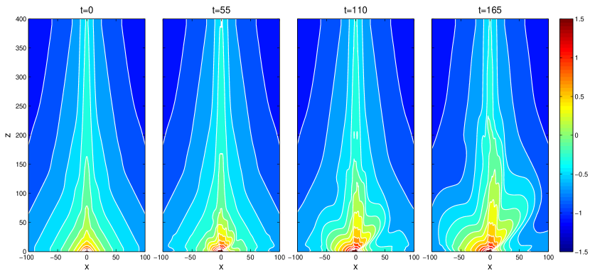
Figure 1: Distributions of column density (log scale) in the $y$ direction at four representative times, with 5 contours per decade. The inner contours for the last two times appear nearly identical, signaling the approach to a steady state.

We perturb the initially steady axisymmetric wind through the boundary conditions on the disk between $\varpi_{g}\leq\varpi\leq\varpi_{0}$. We increase the mass loading rate (through the density at the base of the wind) by a factor of $\sqrt{10}$ on one half of the disk ($x\geq 0$) and decrease it by the same factor on the other half ($x<0$). This perturbation is initiated at $t=0$, and is kept throughout the simulation. The goal is to determine whether the large non-axisymmetric perturbation imposed at the launching surface can lead to disruption of the wind during its acceleration and initial phase of propagation, particularly by the kink ($m=1$) mode. The numerical results are shown in Figs. 1 and 2.

Fig. 1 shows the snapshots of column density in the $y$ direction at four representative times, in units of the radius divided by the Keplerian speed at $\varpi_{g}$. (In this unit, the rotation period at the inner edge of the Keplerian disk is $2\pi$.) At time $t=0$, the column density in the axisymmetric wind is well collimated at large distances along the axis, as predicted by Shu et al. (1995) from asymptotic analysis. As time progresses, an increasingly large portion of the wind becomes distorted as the perturbation propagates outwards from the launching surface. There is no evidence, however, for any growth of instabilities that are commonly expected for such a toroidally dominated wind. Indeed, the perturbed region appears to settle quickly into a nonaxisymmetric steady state, as can be seen by comparing the column density contours in the inner parts of the last two frames.

Fig. 2 displays selected properties of the apparent steady state. In the upper panels, we show the distributions of volume density in an $xy$-plane at height $z=30$ and in an $xz$-plane at $y=0$ for the time $t=165$, corresponding to $26.3$ times the rotation period at the inner edge of the Keplerian disk. Clearly, the density distribution is strongly asymmetric. In the $xy$-plane, it is dominated by a trailing spiral arm outside the central region – the region occupied by the non-magnetocentrifugal outflow injected near the axis (termed “the axial column” hereafter). The spiral is created by the smearing of the denser material magnetocentrifugally launched from one half of the disk surface by rotation. Wind rotation is evident from the velocity vectors displayed, particularly in the central region where the velocity field is dominated by rotation rather than outflowing motion. Inside the axial column, there is some hint of a 4-armed spiral structure in density distribution. We believe the structure is numerical in origin, since the conditions at the base of the axial column are kept axisymmetric. Most likely, it is generated by the rectangular grid, which is not ideal for following rotating motion near the axis. Nevertheless, the numerical artifact appears localized inside the axial column. Between the column and the surrounding magnetocentrifugal wind lies a shell of high density. Most likely, it is created by the squeezing of the strong toroidal magnetic field in the magnetocentrifugal wind against the strong poloidal field in the column. The compressed shell is evident in the density distribution in the $xz$-plane. The shell, which encases the axial column, is tilted away from the $z$-axis. The dense ridge further to the right of the axis (at an angle $\sim 45^{\circ}$) corresponds to the large-scale spiral arm in the $xy$-plane, which has a helical shape in 3D.

The strong asymmetry in mass distribution all but disappears in the distribution of magnetic field, as shown in the lower panels of Fig. 2. In the $xy$-plane, contours of constant total field strength form nearly concentric rings. Close inspection shows that the rings are shifted slightly in the positive $x$ direction. The white contour near the center marks the location where $B_{z}=(B_{x}^{2}+B_{y}^{2})^{1/2}$. Roughly speaking, it divides the axial column of non-magnetocentrifugal outflow (inside the contour) where the magnetic field is mainly poloidal from the toroidally dominated magnetocentrifugal part of the wind; the latter occupies most of the space. The bending of the axial column can be seen more clearly in the $xz$-plot. Except for the narrow region inside the white contour, the magnetic field is toroidally dominated, including the launching surface. The much more symmetric field distribution indicates that the mechanical structure of the steady wind is controlled to a large extent by magnetic stresses, rather than forces due to fluid motions.

3 Discussion: a Built-in Stabilizer for Magnetocentrifugal Winds?

The magnetocentrifugal wind in our simulation appears stable in 3D. There is no evidence for rapid growth of instabilities that would lead to flow disruption, despite the fact that the magnetic field in the wind is toroidally dominated all the way to the launching surface. In particular, there is not hint of exponential growth of the kink ($m=1$) mode, even though our perturbation at the base of the wind is designed to maximize the $m=1$ component. The same conclusion appears to hold for the more lightly loaded winds that we have done as well (see also Krasnopolsky, Li, & Blandford 2003b), although in these cases we are unable to run the simulations for as long.

The most likely reason for the stability is that, in our simulations, the perturbed magnetocentrifugal part of the wind encloses a (light) fast-moving outflow near the axis with a poloidally dominated magnetic field. Mathematically, the fast axial flow is used to provide a clean inner boundary to the outer part of wind driven through the magnetocentrifugal mechanism, which fails close to the axis because of unfavorable field line inclinations. Physically, it may represent a flow driven non-magnetocentrifugally along open field lines anchored on young stars, perhaps by nonlinear Alfvén waves generated through magnetic footpoint motions (e.g., Suzuki & Inutsuka 2005). A magnetically dominated stellar outflow is also seen in the simulations of Ustyugova et al. (2006) for disk-magnetosphere interaction in the “propeller” regime. One may attempt to test the supposition by removing the poloidally dominated fast outflow in the axial region. However, if we were to do this, the field line originally at the interface between the inner flow and outer wind would bend inwards, pulling the field lines right outside of it to a more vertical position. The magnetocentrifugal mechanism would shut off for these field lines, leaving them loaded with little material. A more tenuous outflow may still be possible along these unfavorably inclined field lines, driven for example by Alfvén waves. We would then be back to essentially the original configuration: namely, a lighter and perhaps faster flow dominated by poloidal magnetic field enclosed by a more heavily loaded wind that becomes increasingly toroidally dominated at large distances. Our simulations suggest that the same lightly loaded, nearly vertical field lines that force the open field lines further out on the disk to bend by more than 30^∘ away from the axis to make the magnetocentrifugal wind-launching possible in the first place may stabilize the launched wind at the same time. In other words, if a wind is driven magnetocentrifugally, its stability may be guaranteed by the built-in stabilizer. This two-component structure is intrinsic to the X-wind theory, where the stabilizer is envisioned as the open stellar field (Ostriker & Shu, 1995). The same stabilizing mechanism should work equally well, if not better, in the disk-wind picture where, in addition to the stellar field, lightly loaded field lines on the inner part of the disk can also contribute to wind stabilization, especially if there is magnetic flux accumulation due to disk accretion.

Our simulations are limited to the region of acceleration and early propagation of magnetocentrifugal winds, where they appear stable. Whether such winds can stably propagate to much larger distances remains to be determined. Kink instabilities are seen in some simulations of MHD jet propagation (e.g., Nakamura & Meier 2004). The adopted jets are different from the magnetocentrifugally driven jet in our picture, which is simply the densest part of a space-filling wind that also includes an inner, axial region dominated by a poloidal magnetic field and an outer, more tenuous wide-angle component (Shu et al., 1995). We have treated the disk as a fixed boundary. Allowing the disk to evolve in response to angular momentum removal by the wind may lead to instability in the coupled disk-wind system (Lubow, Papaloizou, & Pringle 1994; see, however, Königl 2004). We plan to address this important issue in the future through numerical experiments.

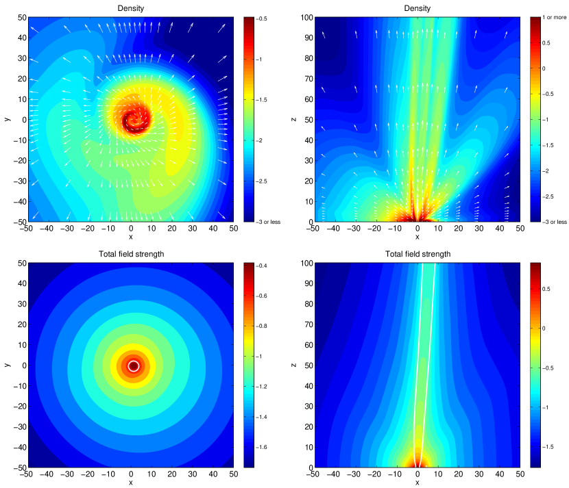
Figure 2: Properties of the non-axisymmetric steady state. Upper panels show the density distribution (log scale) in an $xy$-plane at height $z=30.14$ (left) and in the $xz$-plane at $y=0$ (right). Superposed are vectors of velocity field in the plane, with the length of arrow proportional to the magnitude of velocity. Lower panels show the distribution of total field strength (log scale) in the same $xy$- (left) and $xz$-plane (right), with white contours marking the location where $B_{z}=(B_{x}^{2}+B_{y}^{2})^{1/2}$. Roughly speaking, the magnetic fields inside (outside) the contours are poloidally (toroidally) dominated.

References

- Anderson et al. (2005) Anderson, J. M, Li, Z.-Y., Krasnopolsky, R. & Blandford, R. D. 2005, ApJ, 630, 945
- Appl & Camenzind (1992) Appl, S., & Camenzind, M. 1992, A&A, 256, 354
- Baty & Keppens (2002) Baty, H., & Keppens, R. 2002, ApJ, 580, 800
- Begelman (1998) Begelman, M. C. 1998, ApJ, 493, 291
- Blandford & Payne (1982) Blandford, R. D., & Payne, D. G. 1982, MNRAS, 199, 883
- Bodo et al. (1998) Bodo, G., Rossi, P., Massaglia, S., Ferrari, A., Malagoli, A., Rosner, R. 1998, A&A, 133, 1117
- Clarke, Norman, & Fiedler (1994) Clarke, D. A., Norman, M. L., & Fiedler, R. A. 1994, ZEUS-3D User Manual (Tech. Rep. 015; Urbana-Champaign: National Center for Supercomputing Applications)
- Edwards et al. (2006) Edwards, S., Fischer, W., Hillenbrand, L. & Kwan, J. 2006, ApJ, 646, 319
- Eichler (1993) Eichler, D. 1993, ApJ, 419, 111
- Ferrari (1998) Ferrari, A. 1998, ARA&A, 36, 539
- Hardee (2004) Hardee, P. E. 2004, Ap&SS, 293, 117
- Heyvaerts & Norman (1989) Heyvaerts, J., & Norman, C. 1989, ApJ, 347, 1055
- Kigure & Shibata (2005) Kigure, K. & Shibata, K. 2005, ApJ, 634, 879
- Königl (2004) Königl, A. 2004, ApJ, 617, 1267
- Krasnopolsky, Li, & Blandford (1999) Krasnopolsky, R., Li, Z.-Y., & Blandford, R. 1999, ApJ, 526, 631
- Krasnopolsky, Li, & Blandford (2003a) Krasnopolsky, R., Li, Z.-Y., & Blandford, R. 2003a, ApJ, 595, 631
- Krasnopolsky, Li, & Blandford (2003b) Krasnopolsky, R., Li, Z.-Y., & Blandford, R. 2003b, Ap&SS, 287, 75
- Lery, Baty, & Appl (2000) Lery, T., Baty, H., & Appl, S. 2000, A&A, 355, 1201
- Lubow, Papaloizou, & Pringle (1994) Lubow, S., Papaloizou, J., & Pringle, J. 1994, MNRAS, 268, 1010
- Lucek & Bell (1996) Lucek, S. G., & Bell, A. R. 1996, MNRAS, 281, 245
- Lucek & Bell (1997) Lucek, S. G., & Bell, A. R. 1997, MNRAS, 290, 327
- Nakamura & Meier (2004) Nakamura, M., & Meier, D. L. 2004, ApJ, 617, 123
- Ostriker & Shu (1995) Ostriker, E. C. & Shu, F. H. 1995, ApJ, 447, 813
- Ouyed & Pudritz (1999) Ouyed, R., & Pudritz, R. E. 1999, MNRAS, 309, 233
- Ouyed, Clarke, & Pudritz (2003) Ouyed, R., Clarke, D. A., & Pudritz, R. E. 2003, ApJ, 582, 292
- Shu et al. (1995) Shu, F. H., Najita, J., Ostriker, E. & Shang, S. 1995, ApJ, 455, L155
- Spruit (1996) Spruit, H. C. 1996, Evolutionary Processes in Binary Stars, NATO ASI Series C., 477, 249
- Suzuki & Inutsuka (2005) Suzuki, T. & Inutsuka, S. 2005, J. Geophys. Res., 111, A06101, doi:10.1029/2005JA011502
- Uchida & Shibata (1985) Uchida, Y. & Shibata, K. 1985, PASJ, 36, 105
- Ustyugova et al. (2006) Ustyugova, G. V., Koldoba, A. V., Romanova, M. M. & Lovelace, R. V. E. 2006, ApJ, 646, 304