GaaP: PSF- and aperture-matched photometry using shapelets

Abstract

Aims. We describe a new technique for measuring accurate galaxy colours from images taken under different seeing conditions.

Methods. The method involves two ingredients. First we define the Gaussian-aperture-and-PSF flux, which is the Gaussian-weighted flux a galaxy would have if it were observed with a Gaussian PSF. This theoretical aperture flux is independent of the PSF or pixel scale that the galaxy was observed with. Second we develop a procedure to measure such a ‘GaaP’ flux from observed, pixellated images. This involves modelling source and PSF as a superposition of orthogonal shapelets. A correction scheme is also described, which approximately corrects for any residuals to the shapelet expansions.

Results. A series of tests on simulated images shows that with this method it is possible to reduce systematic errors in the matched-aperture fluxes to a percent, which makes it useful for deriving photometric redshifts from large imaging surveys.

1 Introduction

Accurate measurement of colours of astronomical sources is important for many applications. In this paper we describe a new technique for colour measurement that is specifically geared towards poorly-resolved galaxy images in wide-area optical surveys. It is often the case that images taken through different filters have different image quality (different seeing or pixel scale, for example), and it is important to correct the photometry for these effects. An important application is the measurement of photometric redshifts of galaxies (e.g., Baum Baum1957 (1957)) from multi-band imaging surveys such as SDSS (Adelman-McCarthy et al. sdssdr4 (2006)), FIRES (Labbé et al. fires1 (2003); Förster Schreiber et al. fires2 (2006)), FDF (Heidt et al. fdf (2003)), CFHTLS (Brodwin et al. cfhtls3 (2006)), or the up-coming KIDS survey on the VST (Kuijken et al., in preparation).

Ideally, the total flux for each source can be measured in each band, after which the colours follow simply. But in practice we are limited to measuring aperture fluxes, because of pixel noise and confusion by neighbouring sources. Finite aperture fluxes are affected by smearing by the point spread function (PSF) and by pixellation.

To measure accurate colours does not require good measurements of the total flux of a source: it is sufficient to determine the flux of a particular intrinsic part of the source in different wavelength bands, and compare those. The aperture need not have sharp edges: any weight function will do. The technical problem to solve is then how to make sure that the same intrinsic part of the source is measured in each band, when all that is available is a set of convolved images of the source, each with a different PSF.

An often-used solution is to smooth all images to the same effective PSF. This involves convolution of the sharpest images in a multi-band set with appropriate convolution kernels, resulting in smoothed images that have the same PSF as the worst-seeing image of the set. Matched-aperture photometry on these images then yields proper colours. A practical disadvantage of this method is that all images need to be brought together in order to compute the proper convolution kernels—in case of a large multi-band survey this is not a simple task. It is also computationally expensive to convolve all pixels of an image with a spatially variable kernel, particularly if most of these pixels will in the end not be part of any source.

This paper describes a different approach which is considerably more efficient and no less accurate. Rather than convolving images to each other’s PSF, we encode the detected sources in each image as a sum of orthogonal basis functions (‘shapelets’, Refregier Refregier2003 (2003), henceforth R03). The same is done for the PSF. From this point on we only manipulate the sources, removing the need to convolve all pixels. For each source we then construct a ’PSF cleaning’ operator with which to compute the aperture flux that would be measured with a standard (Gaussian) PSF. By standardizing on a ’clean’ PSF we avoid the need to know the ’dirty’ PSFs of all bands at once, which means that images can be analysed quite independently.

This paper is organized as follows. Section 2 defines the aperture flux we will use. Section 3 summarizes the shapelets formalism, and we show there how to use it to compute our aperture fluxes for shapelet objects. An error analysis is also given. In section 4 we present the results of many simulations, and derive several technical improvements which take into account the residuals to the shapelet description for the observed sources and PSFs. Tests of the noise propagation and a discussion of the choice of aperture radius are treated in section 5. After a short discussion (Section 6) we summarize the paper in Section 7.

2 An aperture flux measure independent of PSF

We define the ’Gaussian-aperture-and-PSF’ (GaaP) flux $F_{q}$ of aperture radius $q$ as the Gaussian-weighted flux the source would have if it were observed with a Gaussian PSF of the same width as the weight function:

$$F_{q}\equiv\int d{\bf r}\,e^{-r^{2}/2q^{2}}\int d{\bf r^{\prime}}S({\bf r^{\prime}}){e^{-({\bf r}-{\bf r^{\prime}})^{2}/2q^{2}}\over 2\pi q^{2}}$$ (1)

where $S$ is the intrinsic (pre-PSF, pre-pixelization) light distribution of the source. We will show below how we can estimate $F_{q}$ from observed (PSF-convolved, pixelated) images of the source.

Changing the order of integration in eq. 1 and some simple algebra shows that $F_{q}$ is equivalent to the integral

$$F_{q}=\int d{\bf r}\,\frac{1}{2}e^{-r^{2}/4q^{2}}S({\bf r}),$$ (2)

i.e., half of the weighted flux of the intrinsic source $S$ with a Gaussian weight function of dispersion $2^{1/2}q$.

The GaaP flux for Sersic model light profiles is plotted in Fig. 1, and compared with the top-hat aperture flux. As expected (because the GaaP flux includes some smoothing), the GaaP flux has a flatter curve of growth than the straight aperture flux, and is less sensitive to differences in galaxy type.

Figure 1: Left: The GaaP aperture flux for different Sersic profiles of effective radius 1, and total flux 1, as a function of aperture radius $q$. From steepest to flattest, Sersic index 0.5 (Gaussian), 1 (exponential), 2, 3 and 4 (de Vaucouleur) are plotted. Right: the top-hat aperture fluxes within radius $q$ for the same profiles.

3 Shapelets

In the shapelets formalism (R03) images are expressed as a truncated sum of orthonormal Gauss-Hermite terms. In this paper we follow the notation used in Kuijken (Kuijken2006 (2006), henceforth K06), where an application of shapelets to weak gravitational lensing is described.

The shapelet basis function of scale $\beta$ and $x,y$ orders $a,b$ is

$$B^{ab}(x,y)=k^{ab}\beta^{-1}e^{-[(x-x_{c})^{2}+(y-y_{c})^{2}]/2\beta^{2}}H^{a}(x/\beta)H^{b}(y/\beta),$$ (3)

where $x_{c}$ and $y_{c}$ are the center of the expansion, $B^{ab}$ is the basis function of order $(a,b)$, $H^{a}$ is the Hermite polynomial of order $a$ and

$$k^{ab}=1/\sqrt{\pi a!b!2^{a+b}}$$ (4)

is a normalization constant chosen so that $\left(B^{ab}\right)^{2}$ integrates to one.

An image of a source, or a point spread function, can be expressed as a sum of such basis functions with coefficients $s_{ab}$. This can be done in two, not quite equivalent ways: by integration or by fitting. Integration is more straightforward in principle. The $B^{ab}$ are an orthonormal basis, so the coefficient of each term is simply the integral of the image times this basis function. Since the image is pixellated, however, performing this integral numerically is fundamentally inaccurate since it needs to be approximated by a finite sum. Fitting has the advantage that it is well-defined: one minimizes $\chi^{2}$ over all coefficients, which yields a description of an image that fits the fluxes in each image pixel. Formally, the best-fit coefficients therefore describe the pixel-convolved image, which means that when image and PSF are both fitted in the same way, their deconvolution should be independent of the pixel scale. In this paper we determine shapelet coefficients by least-squares fitting to the pixel values.

Once the shapelet coefficients have been determined they can be operated on to calculate the effects of convolution, translation, magnification, shear, etc, as well as a range of photometric quantities. For the present application the relevant operations are convolution, and weighted-aperture photometry.

Convolution of a source by a PSF is a linear operator and can be represented by the action of a PSF matrix ${\bf P}$. The elements of ${\bf P}$ depend on the shapelet coefficients $p_{ab}$ and scale $\beta_{\mathrm{psf}}$ of the PSF, on the shapelet scale $\beta_{\mathrm{in}}$ of the source being convolved, and on the shapelet scale $\beta_{\mathrm{out}}$ of the result. For a model source whose shapelet coefficients are $m_{ab}$, the convolution with the PSF can be written as

$$\left(\sum_{a,b}p_{ab}B^{ab}_{\beta_{\mathrm{psf}}}\right)\otimes\left(\sum_{a,b}m_{ab}B^{ab}_{\beta_{\mathrm{in}}}\right)\qquad\qquad\qquad$$

$$=\sum_{a_{1},b_{1}}\left(\sum_{a_{2},b_{2}}{\bf P}_{a_{1}b_{1}a_{2}b_{2}}(\beta_{\mathrm{in}},\beta_{\mathrm{out}})m_{a_{2}b_{2}}\right)B^{a_{1}b_{1}}_{\beta_{\mathrm{out}}}.$$ (5)

The coefficients of the PSF matrix are

$${\bf P}_{a_{1}b_{1}a_{2}b_{2}}(\beta_{\rm in},\beta_{\rm out})=\sum_{a_{3},b_{3}}C_{a_{1}a_{3}a_{2}}^{\beta_{\rm out}\beta_{\rm psf}\beta_{\rm in}}C_{b_{1}b_{3}b_{2}}^{\beta_{\rm out}\beta_{\rm psf}\beta_{\rm in}}p_{a_{3}b_{3}}$$ (6)

where the elemental convolution matrix $C_{mnl}^{\beta_{3}\beta_{1}\beta_{2}}$ expresses the convolution of two one-dimensional shapelets of scales $\beta_{1}$ and $\beta_{2}$ as a new shapelet series with scale $\beta_{3}$. A recurrence relation for $C_{mnl}$ is given in R03.

If the image of the source $S$ is expressed as a shapelet series, with scale radius $\beta$, then the GaaP flux defined in §2 can be calculated analytically for each $S=B^{ab}$: only those terms for which the orders $a$ and $b$ are both even contribute, and in this case the $x$ and $y$ integrals in eq. 2 separate as $F_{q}=F_{q}^{a}F_{q}^{b}$ with

$$F_{q}^{a}=\int dx\,\frac{1}{2}e^{-x^{2}/4q^{2}}{H^{a}(x^{\prime}/\beta)e^{-x^{\prime 2}/2\beta^{2}}\over\sqrt{\sqrt{\pi}2^{a}a!\beta}}$$ (7)

which, with the help of the result that, for even $n$,

$$\int_{-\infty}^{\infty}e^{-t^{2}}H^{n}(tx)dt=\sqrt{\pi}{n!\over(n/2)!}(x^{2}-1)^{n/2}$$ (8)

(Abramowicz and Stegun a+s (1972), eq. 22.13.17) reduces to

$$F_{q}^{a}={\pi^{1/4}\beta^{1/2}\over\sqrt{1+\beta^{2}/2q^{2}}}\sqrt{(a-1)!!\over a!!}\left(2q^{2}-\beta^{2}\over 2q^{2}+\beta^{2}\right)^{a/2}.$$ (9)

(where $0!!=1!!=1$ and $n!!=n(n-2)!!$). Hence the Gaussian-aperture, Gaussian-PSF flux of an object with shapelet coefficients $s_{ab}$ at scale $q$ is simply the sum

$$F_{q}(s)=\sum_{a,b\,\,\mathrm{even}}s_{ab}F_{q}^{a}F_{q}^{b}.$$ (10)

To calculate the GaaP flux of an object $S$ observed with PSF $P$, we therefore

1. express both as shapelet series $s_{ab}$ and $p_{ab}$, using scales $\beta$ and $\beta_{\mathrm{psf}}$ respectively;

2. construct the PSF matrix ${\bf P}$ using eq. 6, using the same value $\beta$ as the input and output shapelet scale;

3. calculate the shapelet expansion for the deconvolved image ${\bf P}^{-1}\cdot{\bf s}$;

4. calculate the GaaP flux using eqs. 9 and 10.

The resulting expression is

$$F_{q}=\sum_{a_{1},b_{1}\,\,\mathrm{even}}\ \ \sum_{a_{2},b_{2}}\ \ {\bf P}_{a_{1}b_{1}a_{2}b_{2}}^{-1}F_{q}^{a_{1}}F_{q}^{b_{1}}s_{a_{2}b_{2}}.$$ (11)

From this expression it is also straightforward to calculate the variance of $F_{q}$: for background-limited imaging the standard errors on the $s_{ab}$ are uncorrelated and, because of the normalization of the basis functions, equal to the standard error $\sigma$ on the flux in a pixel. Hence the variance of the GaaP flux is

$$\hbox{Var}\left(F_{q}\right)=\sum_{a_{2},b_{2}}\left(\sum_{a_{1},b_{1}\,\,\mathrm{even}}{\bf P}_{a_{1}b_{1}a_{2}b_{2}}^{-1}F_{q}^{a_{1}}F_{q}^{b_{1}}\right)^{2}\sigma^{2}.$$ (12)

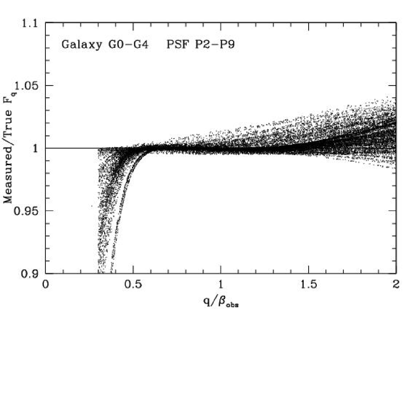
Figure 2: The ratio of the measured GaaP flux to the true value, for a series of simulated Sersic profile model galaxies convolved with Moffat PSF profiles. Models are identified in Table 1. The horizontal axis is the aperture radius $q$, divided by the shapelet scale used to describe the observed image. See the text for details. Shapelet order 8 was used. (Colour versions of this and similar figures indicating the parameter dependence of the results are included in the on-line materials.)

Table 1: PSF and Galaxy profiles used in the tests

PSF type
0	Pseudo-Airy (eq. 23)
1	Pseudo-Airy with 10% spikes
2	Moffat, $m=2$
3	Moffat, $m=3$
9	Moffat, $m=9$ (nearly Gaussian)
Galaxy type
0	Gaussian
1	Sersic, $n=1$ (exponential)
2	Sersic, $n=2$
3	Sersic, $n=3$
4	Sersic, $n=4$ (de Vaucouleur)
5	Spiral (eq. 22)

4 Tests and improvements

To test this procedure, we performed the following simulations. First we generated a series of model galaxy images with Sersic (Sersic1968 (1968)) profiles $\exp(-kr^{1/n})$. These were then convolved with Moffat profile $(1+r^{2}/a^{2})^{-m}$ PSFs, and pixellated to yield simulated images. A corresponding pixellated PSF image was generated in the same way. All images were built by monte-carlo selection, as described in K06.

Each pixelated image and its PSF was then fitted with a shapelet series to order 8. Following K06, we used a scale radius $\beta$ that is 1.3 times the dispersion of the best-fit Gaussian: this choice favours a more accurate description of the outer wings of the images, and helps to suppress any sub-pixel scale freedom the shapelet fit might otherwise have. At this point it is assumed that the correct background level is known; this assumption is addressed in §6.

The GaaP flux is then calculated using eq. 11. and compared with the exact GaaP flux, as calculated directly from eq. 2 and plotted in Fig. 1. We repeated this procedure for a range of aperture radii $q$ for each model, and ran a large set of models of different Sersic index for the galaxies (0.5 to 4), Moffat index for the PSF (2, 3 and 9), galaxy effective radius (from completely unresolved to 6 pixels), PSF FWHM (3 to 6 pixels), and location of the galaxy centre with respect to the pixel grid (center and corner of a pixel, middle of an edge).

The results of this first test are plotted in Fig. 2, which show that, provided the Gaussian aperture radius $q$ is within a factor of two of the shapelet scale of the observed source, the procedure yields GaaP fluxes that are accurate to 10% or better. Going to shapelet order 12 improves the results somewhat (not shown), but not spectacularly.

While useful, these residuals are still troublingly large. We now describe two simple refinements which take account of the residuals to the shapelet fits to observed source and PSF.

4.1 Residuals to the observed source expansion

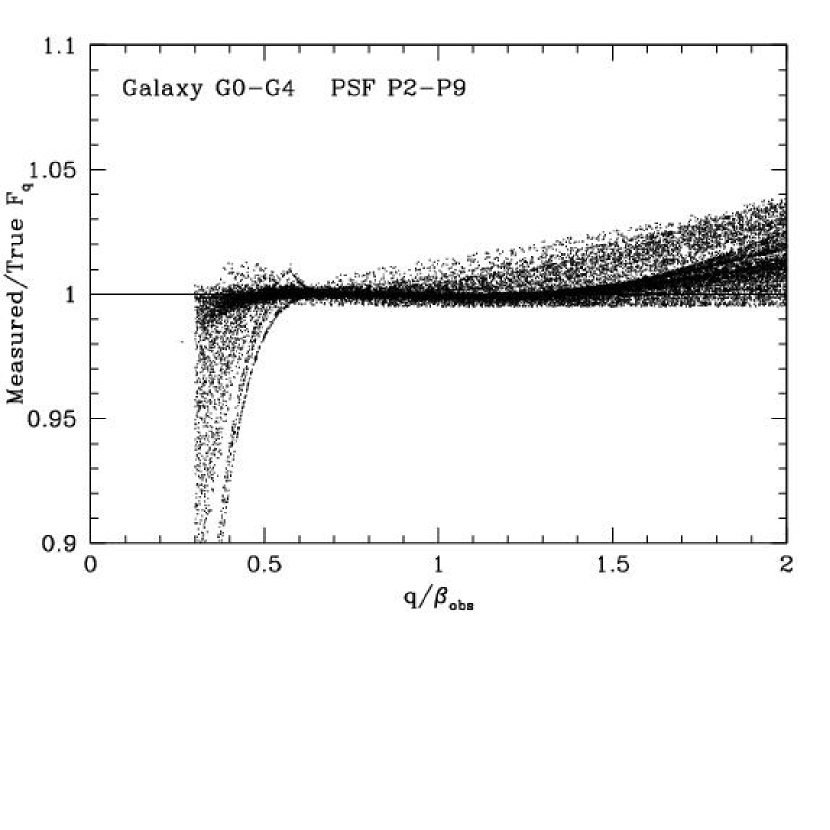
Figure 3: As fig. 2, but now including the additive correction for residual pixel flux to the observed sources’ shapelet expansions.

The first improvement is to take into account the residual galaxy flux $R_{ij}$ at pixel $(i,j)$ to the shapelet expansion:

$$R_{ij}=S^{\mathrm{obs}}(x_{i},y_{i})-\sum_{a,b}s_{ab}B^{ab}(x_{i},y_{j}).$$ (13)

Thus far we have simply ignored this flux, but a better approximation is to include its Gaussian aperture flux (albeit with only an approximate PSF correction) in the total. Approximating the PSF by a Gaussian of dispersion $g_{\mathrm{psf}}$, we can estimate the residual GaaP flux by convolving $R_{ij}$ with a Gaussian of dispersion $(q^{2}-g_{\mathrm{psf}}^{2})^{1/2}$, and computing the Gaussian-weighted aperture flux of this convolution:

$$\int d{\bf r}\int d{\bf r^{\prime}}R({\bf r^{\prime}}){e^{-({\bf r}-{\bf r^{\prime}})^{2}/(2q^{2}-2g_{\mathrm{psf}}^{2})}\over 2\pi(q^{2}-g_{\mathrm{psf}}^{2})}e^{-r^{2}/2q^{2}}$$ (14)

which, after changing the order of integration can be written (as a generalization of eq. 2) as the aperture integral

$$\int d{\bf r}R({\bf r}){q^{2}\over 2q^{2}-g_{\mathrm{psf}}^{2}}e^{-r^{2}/(4q^{2}-2g_{\mathrm{psf}}^{2})}.$$ (15)

Thus we add

$$F_{\mathrm{res}}=\sum_{i,j}R_{ij}{q^{2}\over 2q^{2}-g_{\mathrm{psf}}^{2}}e^{-(x_{i}^{2}+y_{j}^{2})/(4q^{2}-2g_{\mathrm{psf}}^{2})}$$ (16)

to the result obtained from eq. 11. For the simulated Sersic profiles this term can be of order 10% of $F_{q}$, particularly for very peaked images. The effect of incorporating this correction can be seen in Fig. 3.

4.2 Residuals to the PSF model

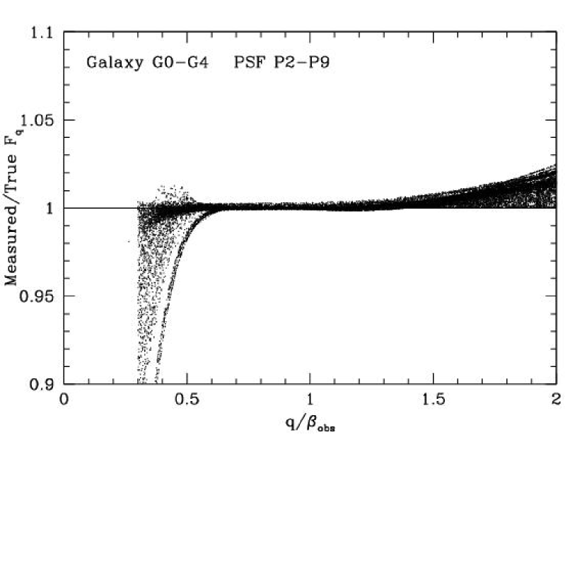
Figure 4: As fig. 3, but now furthermore including the multiplicative correction for residual pixel flux to the PSFs’ shapelet expansions.

The second effect is caused by residuals to the PSF’s shapelet expansion, which can introduce a multiplicative scaling error during the deconvolution. (Essentially, if some of the flux of the PSF is missed in the shapelet model then deconvolution by this underestimated PSF will result in an overestimated galaxy flux.) To estimate the effect of this missed PSF flux, we compute the correction factor for a Gaussian galaxy.

For a Gaussian galaxy, of dispersion $g$ and unit total flux, the GaaP flux $F^{q}$ is equal to (see eq. 2)

$$\int d{\bf r}\,\frac{1}{2}{e^{-r^{2}/2g^{2}}\over 2\pi g^{2}}e^{-r^{2}/4q^{2}}={q^{2}\over 2q^{2}+g^{2}}.$$ (17)

However, if a part $P_{\mathrm{res}}(x,y)$ of the PSF $P$ was not included in the shapelet model, then to first order in these residuals $F_{q}$ will have been overestimated by an amount

$$\int d{\bf r}\,\left[P_{\mathrm{res}}\otimes^{-1}P\otimes G(q)\otimes G(g)\right]e^{-r^{2}/2q^{2}}.$$ (18)

Here $G(\sigma)$ is a Gaussian of dispersion $\sigma$, $\otimes$ denotes convolution and $\otimes^{-1}$ deconvolution. We can estimate this integral by replacing the PSF $P$ by a Gaussian whose dispersion $g_{\mathrm{psf}}$ is chosen to be a reasonable match to the PSF size. Combining all Gaussian (de)convolutions reduces eq. 18 to

$$\int d{\bf r}\,\left[P_{\mathrm{res}}\otimes G\left(\sqrt{q^{2}-g_{\mathrm{psf}}^{2}+g^{2}}\right)\right]e^{-r^{2}/2q^{2}}$$ (19)

or, after the by now customary swapping of the order of integration,

$${q^{2}\over 2q^{2}+g^{2}-g_{\mathrm{psf}}^{2}}\int d{\bf r}\,P_{\mathrm{res}}e^{-r^{2}/(4q^{2}+2g^{2}-2g_{\mathrm{psf}}^{2})}.$$ (20)

The ratio of eqs. 20 and 17 is then an estimate of the fractional error that results from the incomplete PSF model. Correcting for this error is accomplished by dividing $F_{q}+F_{\mathrm{res}}$ (from eqs. 11 and 16) by

$$f_{\mathrm{psf}}=1+{2q^{2}+g^{2}\over 2q^{2}+g^{2}-g_{\mathrm{psf}}^{2}}\int d{\bf r}\,P_{\mathrm{res}}e^{-r^{2}/(4q^{2}+2g^{2}-2g_{\mathrm{psf}}^{2})}.$$ (21)

In practice we estimate $g$, the intrinsic Gaussian size of the source, from the best-fit Gaussian radius of the observed source $g_{\mathrm{obs}}$ as $g^{2}\simeq g_{\mathrm{obs}}^{2}-g_{\mathrm{psf}}^{2}$.

In figure 4 we show the result of implementing these two corrections: the GaaP flux is now systematically correct to better than 2%, over a wide range of Sersic index and PSF size, and for GaaP aperture radii between half and twice the shapelet scale of the observed images. The error is below 1% for $0.6<q/\beta<1.6$, with the worst errors arising for PSFs and galaxies that are only a few pixels across.

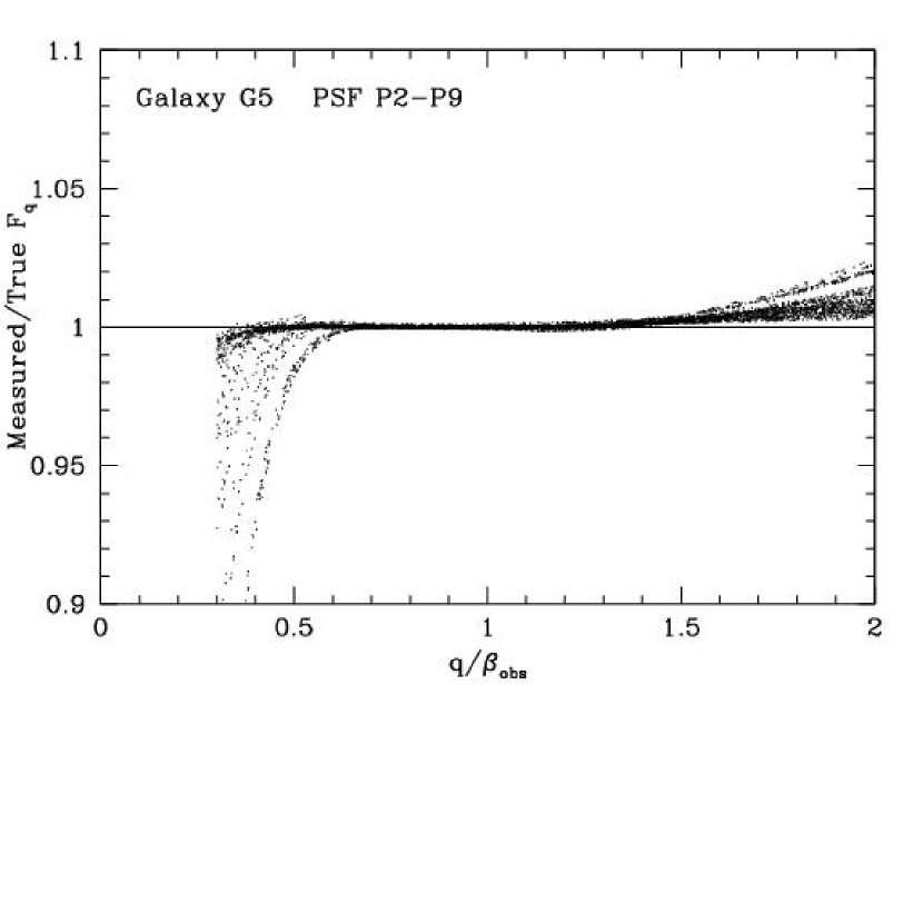
Figure 5: As Fig. 4, but for a two-armed spiral galaxy

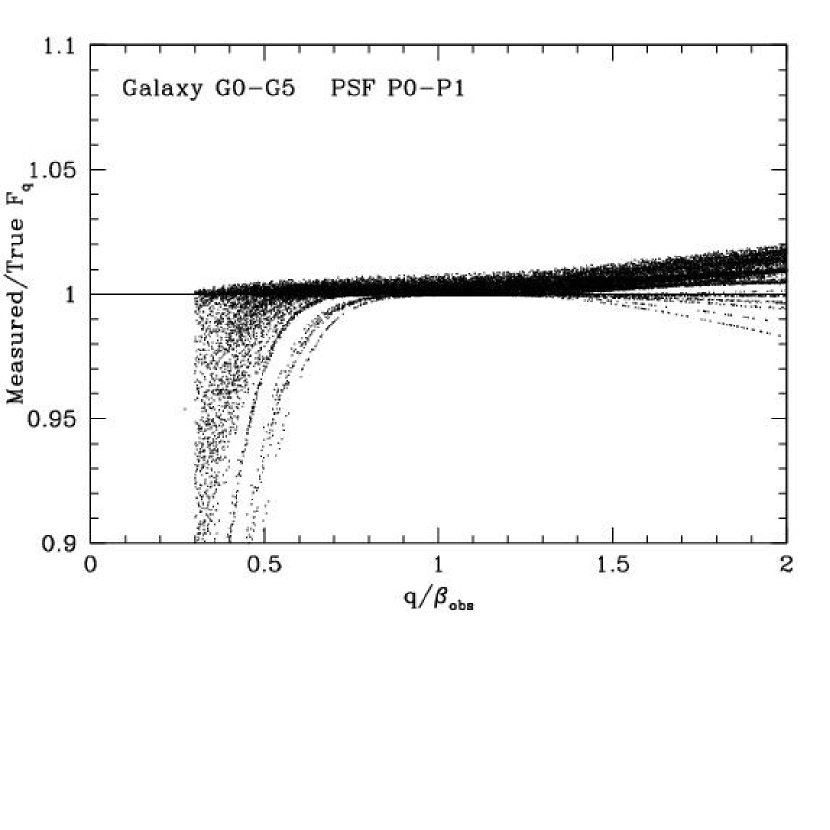
Figure 6: As Fig. 4, but for PSFs with diffraction rings. PSFs 0 and 1 are the same except that PSF 1 includes four diffraction spikes which together contain 10% of the flux.

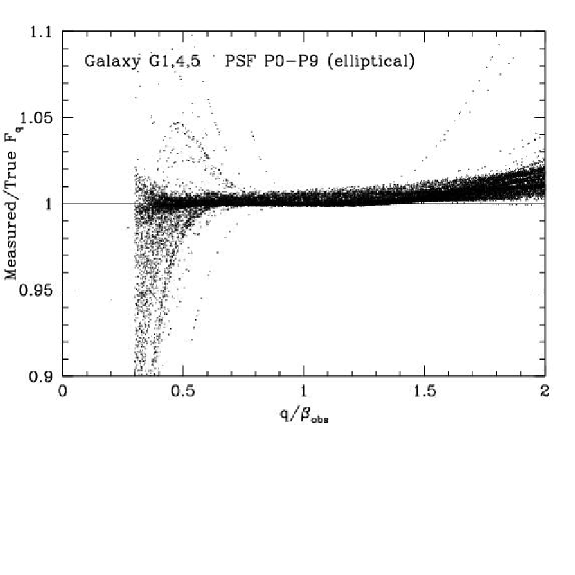
Figure 7: As Fig. 4, but for elliptical PSFs of axis ratio 3:2. PSF and galaxy types have the same meaning as before.

Figure 8: Azimuthally averaged profiles of the PSF (left) and galaxy (right) models used in the simulations. The PSF models are normalized to have FWHM=2, the galaxy models have effective (i.e., half-light) radius equal to 1.

Figure 9: Contour plots of the models used in the simulations. Top two rows: PSF models 0–9; bottom two rows: Galaxy models 0–5. Contours levels differ by a factor of two. The box sizes are six times the FWHM for the PSFs and twelve times the effective radius for the galaxies. See Table 1 for detailed descriptions of these models.

4.3 More complex morphologies

Having established that the method works for circular, regular galaxies, we extended the tests to more complicated shapes. In Fig. 5 we show the $F_{q}$ measurements for a simulated logarithmic spiral galaxy, for the same PSFs as above; the model used is obtained by replacing the random azimuths $\theta$ of stars in a circular exponential disk model by

$$\theta\rightarrow\theta-\frac{1}{2}\cos\left(2(\theta-\ln r)\right).$$ (22)

(The amplitude $\frac{1}{2}$ is chosen to give maximally sharp spiral arms.)

In Fig. 6 we show the results for all galaxy models and with two PSFs that mimick diffraction-limited PSFs. PSF type 0 is defined as

$$\mathrm{PSF0}(r)=\left\{\begin{array}[]{ll}{\sin^{2}r/r^{2}}&\qquad r<1;\\ {\sin^{2}r/r^{3}}&\qquad r>1.\end{array}\right.$$ (23)

and PSF type 1 is the same except that 10% of the flux is put in four thin linear ’diffraction spikes’ along which the density varies as $\mathrm{PSF0}(r/2^{1/2})$. Even here the GaaP flux is recovered to better than 1% for aperture $q$ between 0.7 and 1.5 times $\beta_{\mathrm{obs}}$. In the case where the PSF FWHM is 2 pixels (not shown) the differences can rise to 5%.

Finally, a series of simulations were analysed for circular galaxies that were convolved with elliptical PSFs (axis ratio 3:2). Also here, the results are satisfactory (see Fig. 7).

We therefore conclude that the method works.

More details of the relation between the residuals and the model parameters are given in colour figures included with the on-line material. We close this section with plots (Fig. 8 and  9) of the PSF and galaxy models used in the simulations, and remark that even though the shapelet formalism is built around a Gaussian ‘parent’ flux distribution, it can be used succesfully to do photometry on much more extended sources. Nevertheless, it may be profitable to consider expansions around more galaxy-like parent functions in the future.

Figure 10: Top: The scatter in measured GaaP fluxes from simulated images, $\sqrt{\hbox{Var}(F_{q})}/F_{q}$, versus the theoretical prediction of eq. 12. Each point represents a set of 100 noisy realizations of a particular combination of PSF and Galaxy models from Table 1, with aperture radius $q$ between 0.6 and 1.4 times $\beta_{\mathrm{obs}}$. The scatter is adequately predicted for signal-to-noise ratios above about three. Bottom: the average GaaP flux for each set of 100 realizations, versus the rms scatter, showing that there is no noise-related bias in the results.

5 Noise

A similar set of tests can be used to investigate the effect of noise on the GaaP fluxes: we simply add a constant Gaussian noise level to all pixels in simulated galaxy images, as appropriate for background-limited images, and repeat the analysis many times. In Fig. 10 we show the comparison between the errors prediction from eq. 12, and the scatter from a large number of realizations, using the models of Figs. 2 to 6.

For adequately resolved (FWHM 3 pixels or greater), or more Moffat-like, PSFs, the theoretical error bar adequately predicts the scatter in the measurements, and any bias in the results is neglegibly small.

Figure 11: The effect of aperture radius on S/N of the GaaP fluxes and colours. The thin solid curves show the S/N of the GaaP flux of an exponential disk, $R_{e}=2$ pixels, convolved with Moffat $\beta_{m}=3$ PSFs of FWHM 3 and 6 pixels (top and middle curves—tick marks indicate the shapelet scale radius used to model the sources). The heavy line shows the S/N of the ratio of the fluxes. For this calculation is was assumed that both images have the same pixel noise of 1% of the total flux of the galaxy. The dashed line shows the same result for a de Vaucouleur model galaxy.

Deconvolution will always amplify photon noise, so it is important to try to choose an optimal aperture radius. This is addressed in Fig. 11, which shows how the S/N of the Gaap fluxes and of their ratio varies with aperture radius. In this calculation we assume that a galaxy is observed with PSFs of two different sizes, so that a given choice of aperture radius $q$ requires a different degree of (de)convolution. The ratio of the two GaaP fluxes at a given $q$ represents a colour measurement, with the S/N ratios on the fluxes adding in inverse quadrature. As the figure shows, there is an optimal aperture to use, but the maximum is quite broad, so that useful colours can be measured for a wide range of $q$. It certainly is not optimal to smooth the best-seeing image to the worst one.

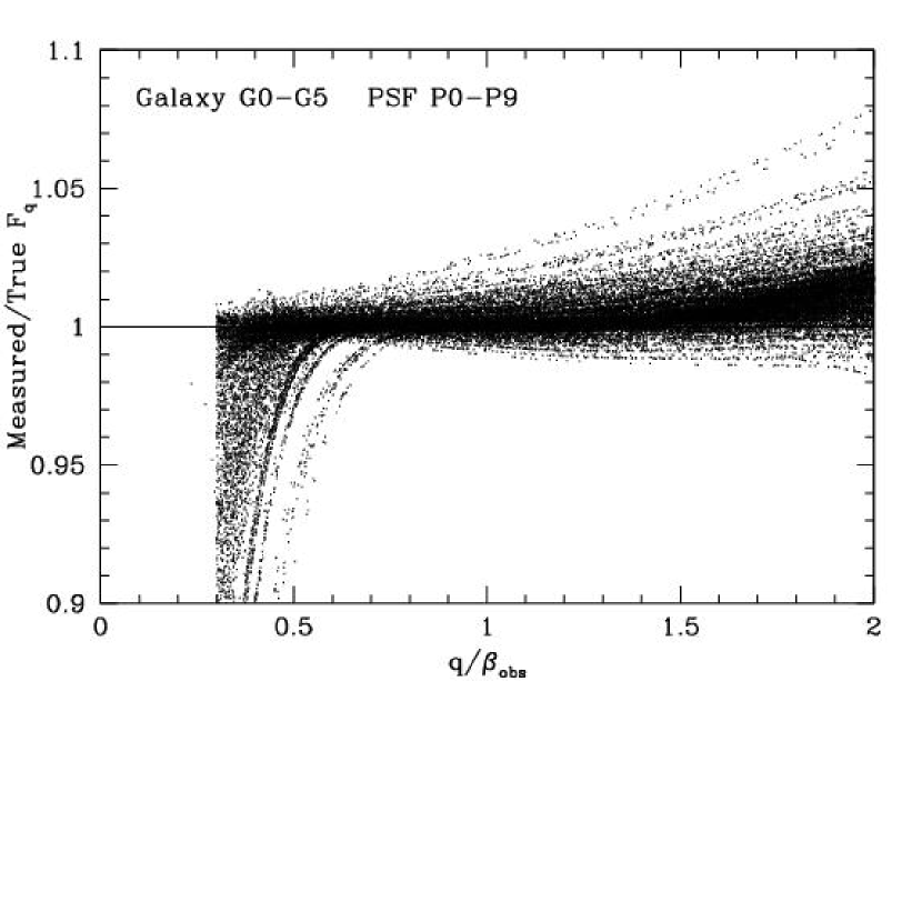
Figure 12: The same simulation as in Fig. 4, except that before the shapelet fitting a locally-fitted background level, determined from an annulus between radius $8\beta$ and $11\beta$ is subtracted. Particularly the ’wingy’ PSFs 0, 1 and 2 are affected by this background error.

6 Discussion

We have shown that the proposed technique is an effective way to generate well-defined aperture fluxes, with accurate error estimates, that are independent of PSF and pixel scale of the observations. In all cases with PSFs that are well-resolved (FWHM at least 3 pixels) systematic errors are below a percent.

The advantage of this approach is that it allows multi-colour photometry to be done on a distributed dataset. All that is needed is a set of object coordinates and aperture radii, and PSF models for each image: then tables of GaaP fluxes can be extracted from each separate image and simply merged into a multi-colour catalogue. The ratios of the GaaP fluxes of aperture radius $q$ are then true integrated colours, corresponding to the ratio of the Gaussian-weighted fluxes of the intrinsic sources with the same weight function $\exp(-r^{2}/4q^{2})$. It should be stressed that the GaaP fluxes are not total fluxes.

This method does not absolve one from knowing the correct background level and zeropoint of each image. This can be difficult with extended galaxies and PSFs, and any flux that is missed in either will have repercussions for the measured aperture fluxes. Provided the images are well flat-fielded, it is possible to obtain decent local background estimates in annuli around each source or star. This will include some source flux from the wings of the flux profile, but for sufficiently large annuli the effect is small. We have tested the effect with the simulations described in §4, by subtracting a background level (determined as the median flux in the pixels between $8\beta$ and $11\beta$ from the centre of the source) before performing the shapelet decomposition. The resulting GaaP fluxes, including all corrections for pixel residuals, are shown in Fig. 12. Not surprisingly, larger apertures are more affected by background level errors, particularly in the PSF. Overall, while the effect is visible, it is not catastrophic: moreover to first approximation the same amount of ’wing’ will be subtracted in different bands so that the overall colours should be affected even less.

We have argued that our procedure is advantageous in the context of large multi-band imaging surveys. The alternative approach of convolving entire images to a common PSF, followed by matched-aperture photometry, is less practical in that it requires much more information exchange between the different images (it may also be more computer-intensive as it requires all pixels to be convolved). In the context of huge multi-band surveys, in which different bands may be observed with different instruments or processed in different places, the logistics of these exchanges are complex.

A different, catalogue-based solution to the problem of deriving accurate colours would be to generate model total fluxes for all sources, e.g. by fitting detected sources to combinations of PSF-convolved Sersic profiles, as done for the Sloan Digital Sky Survey (e.g., Adelman-McCarthy et al. sdssdr4 (2006)). This can also be done image by image, and also yields fluxes that are PSF-independent, but the results will only be valid if the model is appropriate. Few-parameter models are a priori unlikely to yield percent-level accurate total fluxes, and any colour gradients in the source will give rise to wavelength-dependent systematic errors to such a simple fit. By contrast, the method proposed here makes virtually no assumptions on the galaxy shapes.

The technique described in this paper can be used to compare any set of images of a piece of sky: while we have concentrated on colour measurements, another application would be to compare images taken at different epochs to measure time variability. Most time-varying sources are point-like, in which case the more straightforward approach of comparing PSF-fitting fluxes might be more appropriate, but a possible application would be variability of embedded point sources such as galactic nuclei or distant supernovae.

7 Summary

We have defined a PSF-independent aperture flux, the GaaP (Gaussian-aperture and PSF) flux, and showed how it can be extracted from astronomical images provided the point spread function is known. An extensive series of tests on simulated images demonstrates that the level of systematic residual is at or below the 1% level, for aperture sizes that are up to a factor of two larger or smaller than the observed source. Implementation of these ideas into robust data processing pipelines will allow accurate colours to be extracted from large wide-field imaging surveys, virtually free from residual PSF and pixel scale effects.

Appendix A Colour-coded residual plots

This Appendix shows the relation between the residuals in $F_{q}$ measurements and the model parameters. The data plotted are identical to those of Figs. 2 to 7, but the points have been colour-coded according to different model parameters. This helps to identify the most discrepent cases.

As a key to the figures, a summary of all PSF and galaxy models tested is given in Table 1.

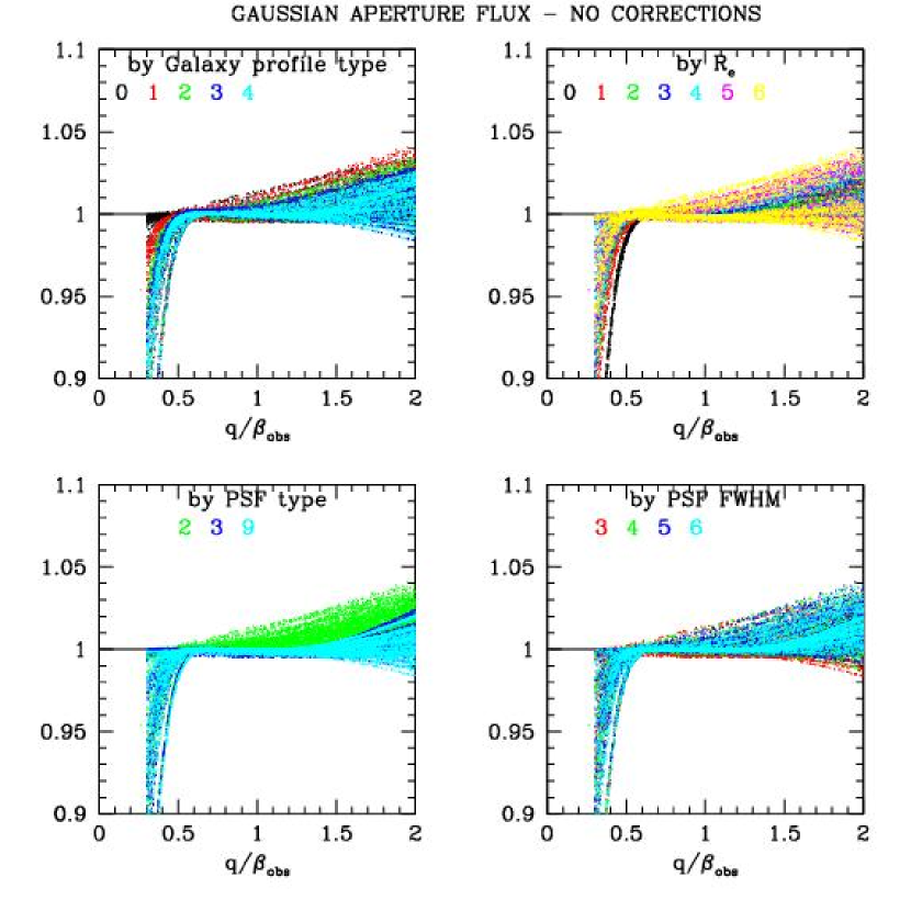
Figure 13: The results of the simulations plotted in Fig. 2, shown here as four panels. Each panel shows the same results, but colour-coded according to a different input parameter: top left, Galaxy type; top right, Galaxy effective radius; bottom left, PSF type; bottom right, PSF FWHM. The colour used to plot the results for each parameter value is shown in each panel, and the model types are identified in Table 1.

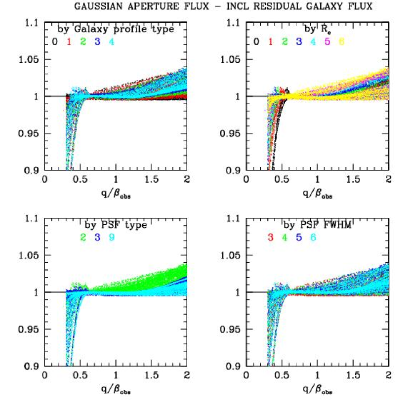
Figure 14: As Fig. 13, but for the results of the simulations plotted in Fig. 3.

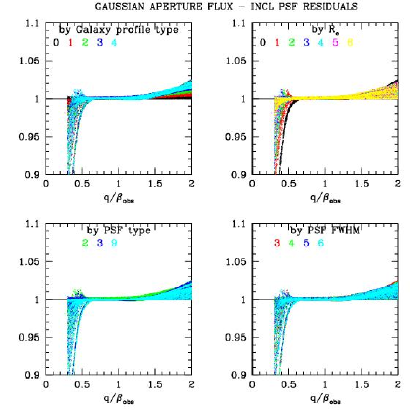
Figure 15: As Fig. 13, but for the results of the simulations plotted in Fig. 4.

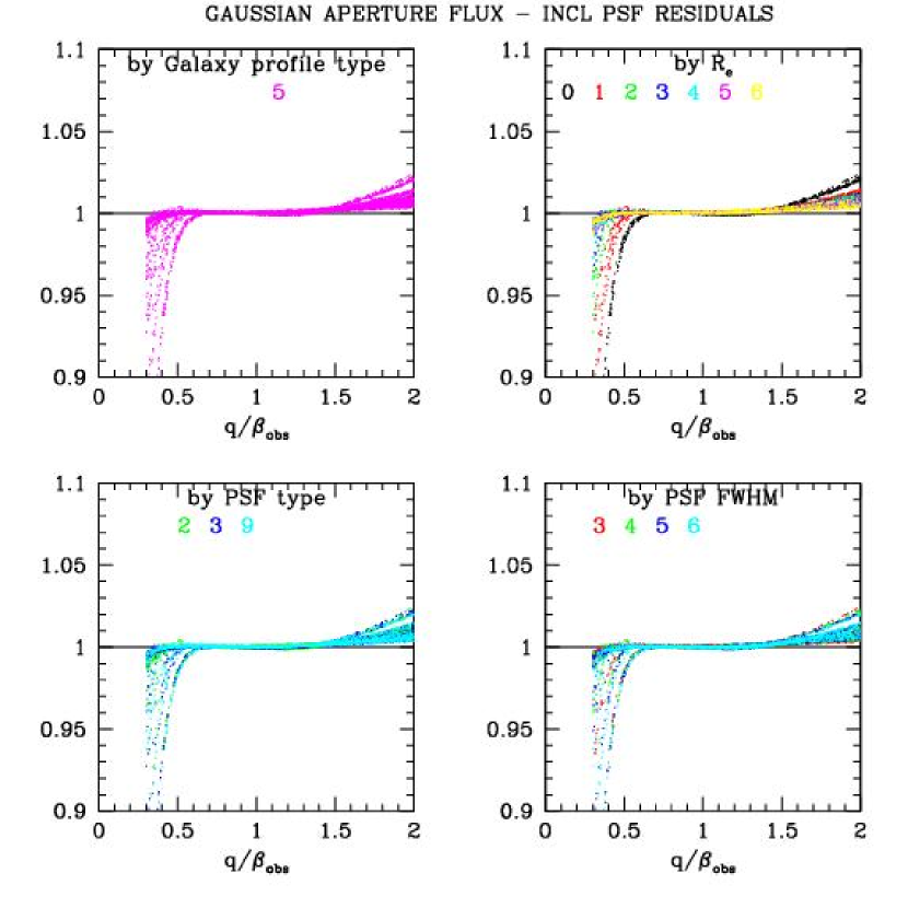
Figure 16: As Fig. 13, but for the results of the simulations plotted in Fig. 5 (spiral galaxy model).

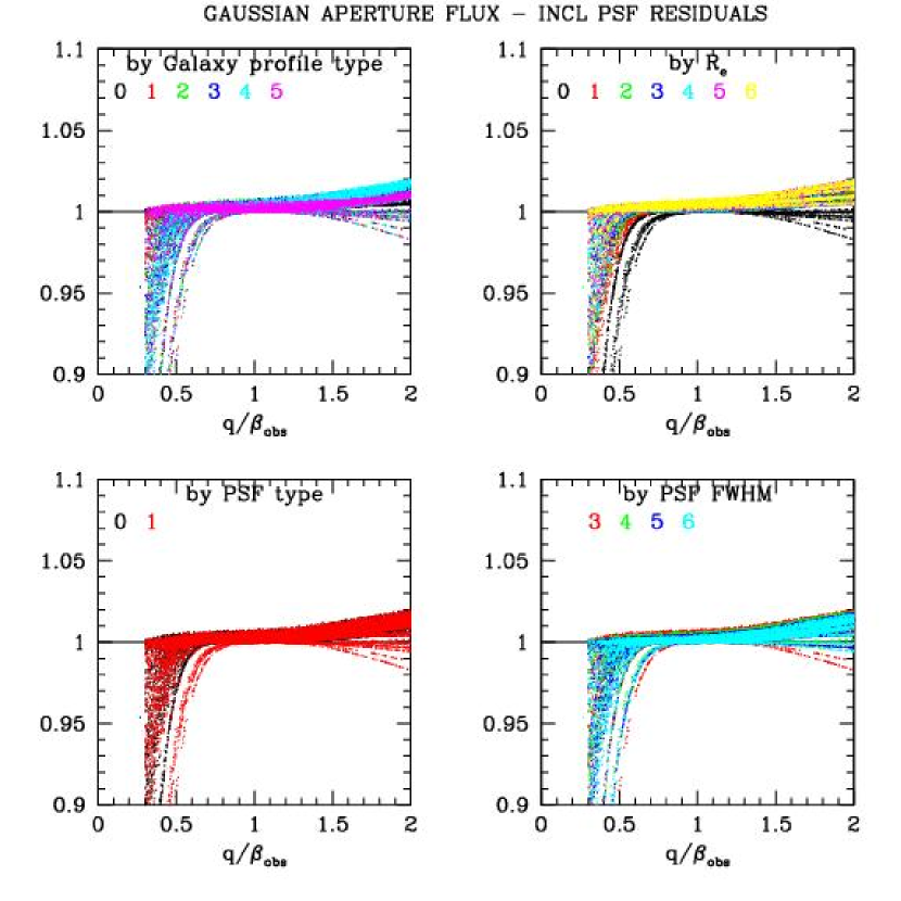
Figure 17: As Fig. 13, but for the results of the simulations plotted in Fig. 6 (Airy function-like PSFs).

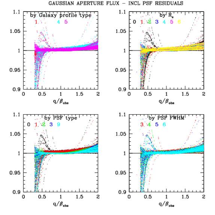
Figure 18: As Fig. 13, but for the results of the simulations plotted in Fig. 7 (elliptical PSFs).

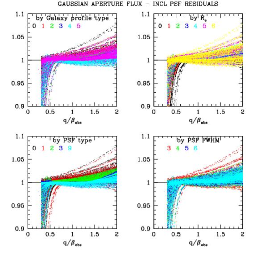
Figure 19: As Fig. 13, but for the results of the simulations plotted in Fig. 12 (locally fitted background subtracted from source and PSF).