Outcome of Six Candidate Transiting Planets
from a TrES Field in Andromeda

Abstract

Driven by the incomplete understanding of the formation of gas giant extrasolar planets and of their mass–radius relationship, several ground–based, wide–field photometric campaigns are searching the skies for new transiting extrasolar gas giants. As part of the Trans-atlantic Exoplanet Survey (TrES), in 2003/4 we monitored approximately 30,000 stars ($9.5\leq V\leq 15.5$) in a $5.7\arcdeg\times 5.7\arcdeg$ field in Andromeda with three telescopes over five months. We identified six candidate transiting planets from the stellar light curves. From subsequent follow-up observations, we rejected each of these as an astrophysical false positive, i.e. a stellar system containing an eclipsing binary, whose light curve mimics that of a Jupiter–sized planet transiting a sun–like star. We discuss here the procedures followed by the TrES team to reject false positives from our list of candidate transiting hot Jupiters. We present these candidates as early examples of the various types of astrophysical false postives found in the TrES campaign, and discuss what we learned from the analysis.

1. Introduction

There are currently 14 extrasolar planets for which we have measurements of both the planetary radius and mass (see Charbonneau et al., 2006, for a review; McCullough et al. 2006; O’Donovan et al. 2006a; Bakos et al. 2006; Collier Cameron et al. 2006). These gas giants have been observed to transit their parent stars, and have supplied new opportunities to study Jupiter–sized exoplanets, in particular their formation and structure. Studies of the visible and infrared atmospheric spectra are possible for the nine nearby ($d<300$ pc) transiting planets (Charbonneau et al., 2002; Vidal-Madjar et al., 2003; Deming et al., 2005a; Charbonneau et al., 2005; Deming et al., 2005b). The incident flux from the closeby ($\mathrel{\hbox to0.0pt{\lower 4.0pt\hbox{\hskip 1.0pt$\sim$}\hss}\raise 1.0pt\hbox{$<$}}0.05\,\mathrm{A.U.}$) star on each of these “hot Jupiters” results in an inflated planetary radius. Current theoretical models that include this stellar insolation can account for the radii of only five of these nine nearby planets. HD 209458 b (Charbonneau et al., 2000; Henry et al., 2000), TrES–2 (O’Donovan et al., 2006a), HAT–P–1 b (catalog HAT-P-1b) (Bakos et al., 2006), and WASP–1 b (catalog WASP-1b) (Collier Cameron et al., 2006) have radii larger than predicted (Laughlin et al., 2005, see and Charbonneau et al. 2006 for reviews of the current structural models for insolated hot Jupiters).The sparse sampling and limited understanding of the mass–radius parameter space for extrasolar planets continue to motivate the search for new transiting planets. There are several small aperture wide–field surveys targeting these objects, such as BEST (Rauer et al., 2004), the HAT network (Bakos et al., 2002, 2004), KELT (Pepper et al., 2004), SuperWASP (Street et al., 2003), Vulcan (Borucki et al., 2001), and XO (McCullough et al., 2005), as well as deeper surveys like the Optical Gravitational Lensing Experiment (OGLE; Udalski et al. 2002) that is probing the Galactic disk.

We are conducting a transit campaign, the Trans-atlantic Exoplanet Survey (TrES), using a network of three 10 cm telescopes with a wide longitudinal coverage: Sleuth (located at Palomar Observatory, California; O’Donovan et al. 2004), PSST (Lowell Observatory, Arizona; Dunham et al. 2004), and STARE (on the isle of Tenerife, Spain; Alonso et al. 2004b). The telescopes monitor over several months a $5.7\arcdeg\times 5.7\arcdeg$ field of view containing thousands of nearby bright stars ($9.5\leq V\leq 15.5$), and we examine the light curves of stars with $V\leq 14.0$ for repeating eclipses with the short–period, small–amplitude signature of a transiting hot Jupiter. We have discovered two transiting planets so far: TrES–1 (Alonso et al., 2004a) and TrES–2 (O’Donovan et al., 2006a). In order to find these two transiting planets, we have processed tens of candidates with light curves similar to that of a sun–like star transited by a Jupiter–sized planet. For a typical TrES field at a Galactic latitude of $b\sim 15\arcdeg$, we find $\sim 10$ candidate transiting planets (Dunham et al., 2004, see, e.g.,). We expect few of these to be true transiting planets, and the remainder to be examples of the various types of astrophysical systems whose light curves can be mistaken for that of a transiting planet (Brown, 2003; Charbonneau et al., 2004, see, e.g.,). These are: low-mass dwarfs eclipsing high-mass dwarfs, giant+dwarf eclipsing binaries, and grazing incidence main-sequence eclipsing binaries (with eclipse depths similar to the $\sim 1$% transit depth of a hot Jupiter); and blends, where a faint eclipsing binary and a bright star coincide on the sky or are physically associated, mixing their light (with the observed eclipse depth reduced to that of a transiting planet). We also encounter occasional photometric false positives, where the transit event is caused by instrumental error, rather than a true reduction in flux from the candidate. Brown (2003) estimates the relative frequency of these astrophysical false positives. For a STARE field in Cygnus, he predicts that from every 25,000 stars observed with sufficient photometric precision to detect a transit, one can expect to identify one star with a transiting planetary companion. However, for this field near the Galactic plane ($b\sim 3\arcdeg$), the number of impostor systems identified as candidate planets will outnumber the true detections by an order of magnitude. (The yield of eclipsing systems from such transit surveys depends on the eclipse visibility, which is the fraction of such systems with a given orbital period for which a sufficient number of eclipses could be observed for the system to be detected. This visibility varies with weather conditions and the longitudinal coverage of the telescopes used.) Of the false positives, approximately half are predicted to be eclipsing binaries and half to be blends.

A careful examination of the light curve of a transit candidate may reveal evidence as to nature of the transiting companion. Seager & Mallén-Ornelas (2003) present an analytic derivation of the system parameters that can be used to rule out obvious stellar systems. If the light curve demonstrates ellipsoidal variability, this indicates the gravitational influence of a stellar companion (Drake, 2003; Sirko & Paczyński, 2003). These tests have been used to great effect on the numerous candidates (177 to date) from the OGLE deep–field survey (Drake, 2003; Sirko & Paczyński, 2003; Pont et al., 2005; Bouchy et al., 2005), and candidates from wide–field surveys (Hidas et al., 2005; Christian et al., 2006, see, e.g.,).

The initial scientific pay-off from each new transiting hot Jupiter comes when an accurate planetary mass and radius have been determined, which can then be used to confront models of planetary structure and formation. These determinations require a high–quality light curve together with a spectroscopic orbit for the host star. For each TrES target field, we follow a procedure of careful examination of each candidate, with follow-up photometry and spectroscopy to eliminate the majority of false positive detections and obtain a high–quality light curve, before committing to the final series of observations with 10-m class telescopes to determine the radial velocity orbit of the candidate planet. This procedure is similar to those discussed by Charbonneau et al. (2004) and Hidas et al. (2005). Here we discuss our follow-up strategy (§2) and present the step–by–step results of this procedure for a field in Andromeda, one of the first fields observed by all three nodes of the TrES network. We describe the TrES network observations in §3, and outline the initial identification of six candidates from the stellar light curves in §4. Based on our follow-up observations of these candidates (§5), we were able to conclude that each was an astrophysical false positive (§6).

2. Follow-up Observations of Planetary Candidates

The light curves from small wide–angle telescopes are not of sufficient quality to derive an accurate radius ratio for the purpose of both false positive rejection and planetary modeling, so high–quality follow-up photometric observations with a larger telescope are needed. Recent experience suggests that a photometric accuracy better than 1 mmag with a time resolution better than 1 minute can be achieved with a meter–class telescope at a good site, and such observations can deliver radius values good to a few percent and transit times good to 0.2 min (Holman et al., 2005, 2006). For smaller telescopes, scintillation can limit the photometric precision at this cadence (Young, 1967; Dravins et al., 1998).

The wide–angle surveys by necessity have broad images, typically with FWHM values of $20\arcsec$. Thus there is a significant probability of a chance alignment between a relatively bright star and a fainter eclipsing binary that just happens to be nearby on the sky. Photometric observations with high spatial resolution on a larger telescope can be used to sort out such cases by resolving the eclipsing binary (Charbonneau et al., 2004, see, e.g.,). In some instances these systems can also be detected using the wide-angle discovery data, by showing that there is differential image motion during the transit events, even though the eclipsing binary is unresolved. Photometry can also be successful in identifying a triple. If the color of the eclipsing binary is different enough from that of the third star, high–quality multi-color light curves will reveal the color–dependent eclipse depths indicative of a such as system (Tingley, 2004; O’Donovan et al., 2006b, see, e.g.,).

A practical problem for this follow-up photometry is that the transiting–planet candidates do not emerge from the wide–angle surveys until late in the observing season, when the observability of the candidates do not permit full coverage of a transit event. With only partial coverage of an event it is difficult to remove systematic drifts across the event, reducing the accuracy of the derived transit depth. Furthermore, full coverage of a transit is important for deriving very accurate transit timings. Without accurate ephemerides, the error in the predicted transit times during the next observing season may be too large to facilitate follow-up photometric observations. The typical duty cycle for a transit is a few hours over a period of a few days, i.e. a few percent. Therefore, if the follow-up photometry does not confirm a transit, the interpretation is ambiguous. The ephemeris may have been too inaccurate, or perhaps the original transit event was a photometric false detection.

One approach to recovering transits and providing an updated ephemeris for high–quality photometric observations with a larger telescope is to monitor candidates with intermediate sized telescopes, such as TopHAT in the case of the HAT survey (Bakos et al., 2004), Sherlock (Kotredes et al., 2004) in the case of TrES, or teams of amateur telescopes (McCullough et al., 2006) in the case of XO.

A second approach to confirming that a candidate is actually a planet is to obtain very precise radial velocities to see whether the host star undergoes a small reflex motion as expected for a planetary companion. This approach has the advantage that the velocity of the host star varies continuously throughout the orbit, so the observations can be made at any time with only modest attention to the phasing compared to the photometric period. The ephemeris can then be updated using the velocities, to provide reliable transit predictions for the follow-up photometry. A second advantage is that a spectroscopic orbit is needed anyway to derive the mass of any candidate that proves to be a planet. The big disadvantage of this approach is that a velocity precision on the order of $10\,\mathrm{m\,s^{-1}}$ is needed, which requires access to a large telescope with an appropriate spectrograph.

For the followup of transiting-planet candidates identified by TrES, we have adopted a strategy designed to eliminate the vast majority of astrophysical false positives with an initial spectroscopic reconnaissance using the Harvard–Smithsonian Center for Astrophysics (CfA) Digital Speedometers (Latham, 1992) on the 1.5-m Wyeth Reflector at the Oak Ridge Observatory in Harvard, Massachusetts and on the 1.5-m Tillinghast Reflector at the F. L. Whipple Observatory (FLWO) on Mount Hopkins, Arizona. We aim to observe candidates spectroscopically during the same season as the discovery photometry. These instruments provide radial velocities good to better than $1\,\mathrm{km\,s^{-1}}$ for stars later than spectral type A that are not rotating too rapidly, and thus can detect motion due to stellar companions with just two or three exposures (Latham, 2003; Charbonneau et al., 2004, see, e.g.,). Thus even if the followup is not performed until the target field is almost setting, we can still reject some candidates spectroscopically, even when photometric followup is not useful. For periods of a few days the limiting value for the mass detectable with these instruments is about 5 to 10 Jupiter masses.

The spectra obtained with these instruments also allow us to characterize the host star. We use a library of synthetic spectra to derive values for the effective temperature and surface gravity, (assuming solar metallicity), and also the line broadening. In our experience, rotational broadening of more than 10 km/s is a strong hint that the companion is a star, with enough tidal torque to synchronize the rotation of the host star with the orbital motion. Although the gravity determination is relatively crude, with an uncertainty of perhaps 0.5 in $\log{g}$, it is still very useful for identifying those host stars that are clearly giants with $\log{g}\leq 3.0$. We presume that these stars must be the third member of a system that includes a main-sequence eclipsing binary, either a physical triple or a chance alignment, and we make no further follow-up observations. Our spectroscopic classification of the host star is a first step towards estimating the stellar mass and radius. These estimates, in turn, may be combined with the observed radial velocity variation and light curve to yield estimates of the mass and radius of the companion.

Although the use of follow-up spectroscopy has the scheduling advantages outlined above, the combination of both spectroscopy and photometry may be needed in the case of a blend. Such a candidate might pass our spectroscopic test as a solitary star with constant radial velocity, if the eclipsing binary of the triple is faint enough relative to the primary star (as was the case for GSC 03885–00829 (catalog GSC 03885-00829); O’Donovan et al. 2006b).

High–precision, high–signal–to–noise spectroscopic observations of the few remaining candidate transiting planets should reveal the mass (and hence true nature) of the transiting companion. However, even after a spectroscopic orbit implying a planetary companion has been derived, care must be taken to show that the velocity shifts are not due to blending with the lines of an eclipsing binary in a triple system (Mandushev et al., 2005, e.g.,). It may be hard to see the lines of the eclipsing binary, partly because the eclipsing binary can be quite a bit fainter than the bright third star, and partly because its lines are likely to be much broader due to synchronized rotation. In some cases it may be possible to extract the velocity of one or both the stars in the eclipsing binary using a technique such as TODCOR (Mandushev et al., 2005). Combining modeling of the photometric light curve and information from the spectroscopic pseudo orbit for the system can help guide the search for the eclipsing binary lines. Even if the lines of the eclipsing binary can not be resolved, a bisector analysis of the lines of the third star may reveal subtle shifts that indicate a binary companion.

Follow-up observations with 1-m class telescopes both remove astrophysical false positives from consideration and prepare for the eventual modeling of newly discovered transiting planets. In the case of our field in Andromeda, our followup ruled out all of our planet candidates, and provided us with a variety of false positives to study.

3. Initial Observations with the TrES Network

In August 2003, we selected a new field centered on the guide star HD 6811 (catalog HD 6811) ($\alpha=01^{\rm h}09^{\rm m}30\fs 13$, $\delta=+47\arcdeg 14\arcmin 30\farcs 5$ J2000). We designated this target field as And0, the first TrES field in Andromeda. We observed this field with each of the TrES telescopes. Although the TrES network usually observes concurrently, in this case weather disrupted our observations. Sleuth monitored the field through an SDSS $r$ filter for 42 clear nights between UT 2003 August 27 and October 24. STARE began its observations with a Johnson $R$ filter on UT 2003 September 17, and observed And0 until UT 2004 Jan 13 during 23 photometric nights. PSST went to this field on UT 2003 November 14 and collected Johnson $R$ observations until 2004 January 11, obtaining 19 clear nights. We estimate our recovery rate for transit events should be 100% for orbital periods $P<6$ days, declining to 70% for $P=10$ days (see Fig. 1), where here our recovery criterion is the observation of at least half the transit from three distinct transit events. We note that this recovery rate is a necessary but not sufficient criterion to detect transiting planets, since it neglects the signal-to-noise ratio and the detrimental effect of non-Gaussian noise upon it (Gaudi et al., 2005; Gaudi, 2005; Pont et al., 2006; Smith et al., 2006; Gaudi & Winn, 2007, see, e.g.,). We used an integration time of 90 s for our exposures. During dark time, we took multicolor photometry (SDSS $g$, $i$, and $z$ for Sleuth and Johnson $B$ and $V$ for PSST and STARE) for stellar color estimates.

4. Searching for Transit Candidates

We have previously described in detail our analysis of TrES data sets in Dunham et al. (2004) and O’Donovan et al. (2006b). We summarize here the analysis for this field. We used standard IRAF (Tody, 1993) tasks or customized IDL routines to calibrate the images from the three telescopes. For each telescope, we derived a standard list of stars visible in the images from this telescope and computed the corresponding equatorial coordinates using the Tycho–2 Catalog (Høg et al., 2000b). We applied differential image analysis (DIA) to each of the separate photometric data sets from the three telescopes, using the following pipeline based in part upon Alard (2000). For each star in our standard star lists, we obtained a time series of differential magnitudes with reference to a master image. We produced this master image by combining 20, 18, and 15 of the best–quality interpolated images in our Sleuth, PSST and STARE data sets, respectively. Since small–aperture, wide–field surveys such as TrES often suffer from systematics (caused, for example, by variable atmospheric extinction), we decorrelated the time series of our field stars.

Initially, we examined our Sleuth observations separately, as these dominate the TrES data set, providing 50% of the data. We binned the Sleuth time series using 9 minute bins to reduce computation time. The rms scatter of the binned data was below 0.015 mag for approximately 7,800 stars. We searched the time series for periodic transit–like dips using the box–fitting least squares transit–search algorithm (BLS; Kovács, Zucker, & Mazeh 2002), which assigns a Signal Detection Efficiency (SDE) statistic to each star, based on the strength of the transit detection. We restricted our search to periods ranging from 0.1 to 10 days. Having sorted the stars in order of decreasing magnitude and decreasing SDE, we visually examined each stellar light curve (phased to the best fit period derived by the algorithm) in turn, until we determined that we could no longer distinguish a transit signal from the noise. We identified six transit candidates (see Tables 1 and 2, and Fig. 3).

We then combined the three TrES data sets, which optimized our visibility function (see Fig. 1), and allowed us to confirm the detection of real eclipse events using simultaneous observations from multiple telescopes. We produced the combined TrES data set as follows. For each star in the Sleuth standard star list, we attempted to identify the corresponding stars in the other two lists. We computed the distances between a given Sleuth standard star and the PSST standard stars, and matched the Sleuth star with a PSST star if their angular separation was less than $5\arcsec$ (0.5 pixels). Because of the slight differences in the chosen filter and field of view, some Sleuth stars did not have corresponding PSST stars. We created a new standard star list from the Sleuth and PSST star lists, with only one entry for each pair of matched stars and an entry for each unmatched star. We then repeated this procedure with this new star list and the STARE list to produce the TrES field standard star list. For each star, we then combined the relevant time series, chronologically reordered the data, and binned the data. The rms scatter of the averaged TrES data was below 0.015 mag for 9,148 stars (see Fig. 2) out of the 29,259 stars in the field. We repeated the BLS transit–search, but did not identify any new candidates. From Figure 1, we can see that a visibility of 80% had already been achieved for $P<5$ d for the Sleuth data alone, and the addition of the STARE and PSST data did not significantly increase the detection space for those short periods. The lack of additional candidates with these orbital periods is not surprising. However, for longer periods, the visibility for the TrES network is much better than for the single Sleuth telescope, yet we did not find new candidates with these periods. We proceeded to our follow-up observations of these six candidates with larger telescopes.

5. Followup of And0 Candidates

Many of the bright stars within our field were also observed as part of other surveys. We identified our candidates in online catalogs and compared these observations with our expectations based on the planet hypothesis. We found Tycho–2 (Høg et al., 2000a, b) visible ($B_{T}-V_{T}$) colors for two of our candidates, and Two Micron All Sky Survey (2MASS; Cutri et al. 2003) infrared ($J-K$) colors for all six (see Tab. 3). We searched the USNO CCD Astrograph Catalog (UCAC2; Zacharias et al. 2004) for the proper motions of the stars. All of the candidates display a measurable proper motion, consistent with nearby dwarfs. However, these proper motions were not sufficiently large to rule out distant, high–velocity giants. Finally, we retrieved Digitized Sky Survey (DSS) images of the sky surrounding each candidate to check for possible nearby stars of similar brightness within our PSF radius. None were found.

We observed the six And0 candidates starting on UT 2004 September 28 using the Harvard–Smithsonian Center for Astrophysics (CfA) Digital Speedometers (Latham, 1992). These spectrographs cover 45Å centered on 5187Å  and have a resolution of $8.5\,\mathrm{km\,s^{-1}}$ (a resolving power of $\lambda/\Delta\lambda\approx 35,\!000$). We cross-correlated our spectra against a grid of templates from our library of synthetic spectra to estimate various stellar parameters of our targets and their radial velocities. J. Morse computed this spectral library, using the Kurucz model atmospheres (J. Morse & R. L. Kurucz, 2004, private communication). Assuming a solar metallicity, we estimated the effective temperature ($T_{\mathrm{eff}}$), surface gravity ($g$) and rotational velocity ($v\sin{i}$) for each candidate (see Tab. 3) from the template parameters that gave the highest average peak correlation value over all the observed spectra.

For the three candidates with low stellar rotation, $v\sin{i}<50\,\mathrm{km\,s^{-1}}$, we obtained several spectra over different observing seasons to determine the radial velocity variation of each star. Table 4 details our spectroscopic observations. For these slowly rotating candidates, the typical precision for our spectroscopic parameters is $\Delta T_{\mathrm{eff}}=150\,\mathrm{K}$, $\Delta\log{g}=0.5$, $\Delta v\sin{i}=2\,\mathrm{km\,s^{-1}}$ and $\Delta V=0.5\,\mathrm{km\,s^{-1}}$. The precision of the estimates degrades for stars with large $v\sin{i}$ values or few spectroscopic observations.

We obtained high precision photometry of T–And0–03874 on UT 2004 December 19 using the Minicam CCD imager at the FLWO 1.2-m telescope on Mt. Hopkins, Arizona. Minicam consists of two 2248$\times$4640 pixel thinned, backside–illuminated Marconi CCDs mounted side–by–side to span a field of approximately 20.4$\times$23.1 arcminutes bisected by a narrow gap. We employed 2$\times$2 pixel binning for an effective plate scale of $0.6\arcsec\,\mathrm{pixel}^{-1}$ and read out each half CCD through a separate amplifier. We offset the telescope to place T–And0–03874 centrally on one amplifier region and autoguided on the field. We obtained concurrent light curves in 3 filters by cycling continuously through the SDSS $g$, $r$, and $z$ filters with exposure times of 90, 45, and 90 seconds respectively. The seeing was poor (FWHM $\sim 3$–$7\arcsec$) and varied throughout our observations. Unfortunately, high winds forced us to close the dome during the night and we obtained only partial coverage of the predicted event. Late in the scheduled observations, we re-opened for a short time.

We subtracted the overscan bias level from each image and divided each by a normalized flat field constructed from the filtered mean of twilight sky exposures. To construct a light curve of T–And0–03874 and neighboring bright stars, we located the stars in each image. We measured stellar fluxes in a circular aperture and subtracted the sky as estimated by the median flux in an annulus centered on the star (iteratively rejecting deviant sky pixel values). We used a relatively large 12$\arcsec$ radius aperture and sky annulus with inner and outer radii of 15$\arcsec$ and 27$\arcsec$ respectively in an effort to reduce systematic errors arising due to the poor and variable seeing conditions. We first corrected the flux of each star by an amount proportional to its airmass in each exposure by using extinction coefficients for each filter based on previous experience with Minicam photometry. Second, we selected a group of bright, uncrowded stars near T–And0–03874 as potential comparison stars. In each exposure, we calculated the mean flux of the comparison stars weighted according to brightness. We assumed that any variations in this mean flux represented extinction in each image and used them to apply corrections to each light curve. We then inspected by eye the light curve of each comparison star, and fit the light curves to models of constant brightness to find chi-squared statistics. We removed from our group of comparison stars any star that showed significant variations. We recalculated the extinction corrections iteratively in this manner until we achieved no variation in the comparison star light curves. We accepted 29, 32, and 4 comparison stars for the $g$, $r$, and $z$ band light curves respectively. Finally, we normalized the flux in the light curves of T–And0–03874 with respect to the out–of–eclipse data.

6. Rejecting False Positive Detections

Based on our detailed investigations of the candidates, we eliminated each And0 candidate as follows.

In the case of T–And0–00948, the TrES light curve (Fig. 3) shows a secondary eclipse. The low surface gravity ($\log{g}=3.0$) is that of a distant giant star, consistent with the red color $J-K=0.60$ (since the majority of stars with $J-K>0.5$ are expected to be giants Brown, 2003, see, e.g.,). There was no observed variation in the radial velocity of this candidate ($v_{r}=-28.82\,\mathrm{km\,s^{-1}}$). T–And0–00948 is most likely the primary star of a diluted triple system.

Upon further examination of the individual light curves for T–And0–01241, we noticed that only Sleuth had observed transit events for this system. Neither PSST nor STARE had observed this field during the time of the Sleuth transit events, preventing a comparison of the light curves. Based on the Sleuth data, we predicted the times of transits during the entire TrES And0 campaign. STARE did observe T–And0–01241 at a time at which it was predicted to transit but did not observe the transit. It was therefore possible that this was a photometric false positive. However, we did not pursue this further, as we obtained sufficient evidence from the follow-up spectroscopy to discount the system. A dwarf with $\log{g}=4.5$, the star has the high effective temperature ($T_{\mathrm{eff}}=9500$ K) and blue colors ($J-K=0.01$) of an early A star. Figure 4$b$ shows the nearly featureless spectrum of this star. For such a large star with a radius $R\sim 2.7\,R_{\sun}$, the observed transit depth of 0.9% indicates a non–planetary size ($R=2.5\,R_{\mathrm{Jup}}$) for the eclipsing body.

The radial velocity of T–And0–02022 varies with an amplitude corresponding to a stellar–mass companion. We determined this system to be an eclipsing binary, comprised of a slightly evolved F dwarf and an M dwarf. This system has a mass function $f(M)=0.0304\pm 0.0013\,\mathrm{M}_{\sun}$ and an eccentricity of $0.027\pm 0.014$. Assuming an orbital inclination of $i\sim 90\arcdeg$, and a mass of $1.6\,\mathrm{M}_{\sun}$ consistent with the effective temperature ($T_{\mathrm{eff}}=7000$ K), we estimated the mass of the companion to be $m=0.5\,\mathrm{M}_{\sun}$. Figure 5 shows the radial velocity orbit. The circular orbit of T–And0–02022 allows us to constrain the stellar radius, independent of our derived spectral type and luminosity class. The circular orbit implies orbital synchronization and orbital–rotation axes alignment, since circularization has the longest timescale of these processes. (This should apply except for very low mass secondaries; Hut, 1981, see for a derivation of these timescales for close binary systems and a comparison for different binary mass ratios and moments of inertia of the primary star.) We can therefore assume that the stellar rotation period is the same as the orbital period of $4.7399$d. We then use the observed rotational broadening ($v\sin{i}=22\,\mathrm{km\,s^{-1}}$) to estimate the radius of the star to be $2.0\,R_{\sun}$. Future photometric observations of this systems with KeplerCam (Szentgyorgyi et al., 2005) are planned to more precisely measure the eclipse depth, and to derive the radius and true mass of each star in this binary (Fernandez et al., in preparation).

T–And0–02462 is a rapid rotator with $v\sin{i}=77\,\mathrm{km\,s^{-1}}$, and displays rotationally broadened lines (see Figure 4$d$), limiting the possibility of detecting the radial velocity variation caused by a planet. Regardless, we implied a binary nature for this candidate using the combined TrES data, which proved essential in identifying this false positive. Our initial Sleuth light curve of T–And0–02462 showed no evidence of a stellar–mass companion, and we derived a BLS best–fit period of 1.5347 d. Upon examining the TrES light curve of T–And0–02462 (see Fig. 3), we noticed a secondary eclipse. Also, the BLS best–fit period for our TrES observations of T–And0–02462 is twice that derived from the Sleuth data alone. When we re-examined the Sleuth data, phased to the TrES period, the secondary eclipse is not visible, due to inadequate coverage at that phase. This resulted in a derived period for the Sleuth data half that of the true period.

The red color of T–And0–03874 ($J-K=0.66$) and the effective temperature ($T_{\mathrm{eff}}=5500$ K) calculated from the spectrum shown in Figure 4$e$ are consistent with an early K–type star. The radial velocity of T–And0–03874 was observed to remain constant at $-15.53\,\mathrm{km\,s^{-1}}$. However, the low estimated surface gravity ($\log{g}=3.5$) suggested this star is a giant star and part of a diluted triple. The photometric follow-up (see Fig. 6) failed to recover transits of T–And0–03874, but did observe a nearby eclipsing binary T–And0–02943 undergoing a deep eclipse at the predicted transit time (also shown in Fig. 6). When we examined our TrES observations for T–And0–02943, we saw that the period of this eclipsing binary was that originally derived for T–And0–03874, namely 2.654 days. This eclipsing system lies $45\arcsec$ away from T–And0–03874, comparable to the PSF radius of our TrES aperture photometry ($30\arcsec$; 3 pixels). The angular resolution ($\sim 1\arcsec\,\mathrm{pixel}^{-1}$) of the 1.2-m photometry is higher than that of the original TrES photometry ($9.9\arcsec\,\mathrm{pixel}^{-1}$); hence the light from these two systems is blended in our TrES observations (see Fig. 7) but is resolved in the 1.2-m photometry.

Finally, the observed parameters for T–And0–03912 ($\log{g}=3.5$, $T_{\mathrm{eff}}=7750$ K, $J-K=0.25$) again imply a large stellar radius ($R\sim 1.8\,R_{\sun}$). In order to produce the 0.9% transit, a companion radius of $1.5\,R_{\mathrm{Jup}}$ is required. This is consistent with the large radii of the transiting planets HAT–P–1 b (catalog HAT-P-1b) (Bakos et al., 2006), and WASP–1 b (catalog WASP-1b) (Charbonneau et al., 2007), although we have not ruled out the possibility of a blend. Regardless, the star T–And0–03912 is rapidly rotating ($v\sin{i}=88\,\mathrm{km\,s^{-1}}$; see Fig. 4$f$), making precise radial-velocity followup extremely difficult.

7. Discussion

The Trans-atlantic Exoplanet Survey monitors $\sim 30,000$ stars each year from which we identify $\sim 30$ stars whose light curves show periodic eclipses consistent with the passage of a Jupiter–sized planet in front of a sun–like star. In order to eliminate astrophysical false positives, we have established a procedure of multi–epoch photometric and moderate–precision spectroscopic follow-up. Surviving candidates are optimal targets for high–precision multi–epoch radial velocity measurements that will yield the masses of planetary companions.

The TrES field in Andromeda was one of the first of our fields for which we combined the data from the three TrES telescopes. We have demonstrated here the benefit of this: the improved transit visibility, the increase in number of stars with low RMS residual, and the confirmation of transit events observed by different telescopes. It has also provided us with several examples of the astrophysical false positives that will be encountered in any ground–based, wide–field transit survey, all of which were rejected as a result of follow-up observations. Based on our experience with these false positives, we refined the criteria by which we identify TrES planet candidates. For each new transit candidate, we now search our dataset for a nearby eclipsing binary with a similar period as derived by the BLS algorithm, in order to check for blends. We also examine the transit light curve phased using integer multiples or fractions of the BLS orbital period.

In comparison to other, more subtle examples (such as those discussed by O’Donovan et al. 2006b, Torres et al. 2004, and Mandushev et al. 2005), these transit candidates were easily identified as false positives. These examples demonstrate the need for both spectroscopic and photometric follow-up of transit candidates, which may be accomplished with the 1-m class telescopes, on which time is readily available. This ensures that the precious resource of 10-m spectroscopy is used efficiently.

Table 1TrES labels for And0 candidate planets, together with corresponding 2MASS and GSC designations and instrumental $V$ magnitude.

Candidate	2MASS	GSC	$V$
T–And0–00948	01083088+4938442 (catalog 2MASS J01083088+4938442)	03272–00845 (catalog GSC 03272-00845)	11.4
T–And0–01241	00531053+4717320 (catalog 2MASS J00531053+4717320)	03266–00642 (catalog GSC 03266-00642)	11.6
T–And0–02022	01023745+4808421 (catalog 2MASS J01023745+4808421)	03267–01450 (catalog GSC 03267-01450)	12.0
T–And0–02462	01180059+4927124 (catalog 2MASS J01180059+4927124)	03272–00540 (catalog GSC 03272-00540)	12.2
T–And0–03874	00545421+4805505 (catalog 2MASS J00545421+4805505)	03266–00119 (catalog GSC 03266-00119)	12.7
T–And0–03912	00595445+4902030 (catalog 2MASS J00595445+4902030)	03271–01102 (catalog GSC 03271-01102)	12.7

Table 2Transit properties for the six TrES And0 candidates.

Candidate	SDE	Depth	Period	Duration	$N$	Telescope(s)	True Nature
		(mag)	(Days)	(Hours)
T–And0–00948	19.3	0.005	1.1198	1.6	7	S,T	Eclipsing binary
T–And0–01241	009.6	0.009	4.6619	3.4	2	S	A–type star
T–And0–02022	13.8	0.017	4.7399	3.4	5	S,P,T	Eclipsing binary
T–And0–02462	21.5	0.019	3.0691	2.2	3	S,P	Eclipsing binary
T–And0–03874	12.7	0.007	2.6540	3.2	7	S,P	Blend
T–And0–03912	18.2	0.007	2.3556	3.4	7	S,P,T	Rapidly rotating A–type star

Table 3Photometric and spectroscopic properties of the six TrES And0 candidates.

Candidate	$v_{r}$	$P(\chi^{2})$	$T_{\mathrm{eff}}$	$\log{g}$	$v\sin{i}$	$\mu$	$B_{T}-V_{T}$	$J-K$
	($\mathrm{km\,s^{-1}}$)		($K$)		($\mathrm{km\,s^{-1}}$)	($\mathrm{\mathrm{mas\,yr^{-1}}}$)	(mag)	(mag)
T–And0–00948	$-28.82\pm\phantom{0}0.53$	0.180	5250	3.0	03	3.0	+$0.87$	$0.60$
T–And0–01241	$-13.05\pm\phantom{0}4.06$	$\cdots$	9500	4.5	55	7.7	$-0.07$	$0.01$
T–And0–02022	$\phantom{string}4.47\pm 27.87$	0.000	7000	3.5	22	3.5	$\cdots$	$0.24$
T–And0–02462	$-11.31\pm\phantom{0}4.73$	0.008	6250	3.5	77	5.5	$\cdots$	$0.14$
T–And0–03874	$-15.41\pm\phantom{0}0.31$	0.747	5500	3.5	02	6.0	$\cdots$	$0.66$
T–And0–03912	$-35.26\pm\phantom{0}3.43$	$\cdots$	7750	3.5	88	8.2	$\cdots$	$0.25$

Table 4Time of observation, orbital phase and radial velocity for spectroscopic observations of the six TrES And0 candidates.

Candidate	Time of Observation	Photometric Orbital Phase	Radial Velocity
	HJD		$\mathrm{km\,s^{-1}}$
T–And0–00948	2453276.8749	0.46	$-28.16\pm 0.36$
$\cdots$	2453277.8530	0.33	$-29.19\pm 0.40$
$\cdots$	2453278.8236	0.20	$-29.00\pm 0.32$
T–And0–01241	2453276.8062	0.73	$-13.05\pm 4.06$
T–And0–02022	2453276.8642	0.80	$\phantom{string}35.46\pm 0.74$
$\cdots$	2453301.8475	0.07	$-14.14\pm 0.99$
$\cdots$	2453334.7734	0.02	$-\phantom{0}3.77\pm 0.94$
$\cdots$	2453548.9711	0.21	$-39.63\pm 1.12$
$\cdots$	2453575.9740	0.90	$\phantom{string}24.54\pm 1.05$
$\cdots$	2453576.9683	0.11	$-20.34\pm 1.16$
$\cdots$	2453626.9029	0.65	$\phantom{string}23.98\pm 1.13$
$\cdots$	2453627.9043	0.86	$\phantom{string}29.37\pm 0.70$
$\cdots$	2453628.8392	0.06	$-\phantom{0}9.31\pm 0.81$
$\cdots$	2453629.8518	0.27	$-42.28\pm 1.12$
$\cdots$	2453630.8361	0.48	$-15.29\pm 1.24$
$\cdots$	2453631.8335	0.69	$\phantom{string}30.93\pm 0.86$
$\cdots$	2453632.8135	0.90	$\phantom{string}24.80\pm 0.87$
$\cdots$	2453633.8047	0.10	$-20.66\pm 1.02$
$\cdots$	2453636.8830	0.75	$\phantom{string}37.44\pm 0.86$
$\cdots$	2453779.5864	0.84	$\phantom{string}29.64\pm 1.14$
T–And0–02462	2453276.8864	0.11	$-\phantom{0}7.55\pm 1.40$
$\cdots$	2453686.7688	0.18	$-14.50\pm 3.74$
T–And0–03874	2453276.8192	0.17	$-15.81\pm 0.44$
$\cdots$	2453277.8381	0.55	$-15.15\pm 0.41$
$\cdots$	2453301.8342	0.59	$-15.09\pm 0.43$
$\cdots$	2453334.7619	0.00	$-15.50\pm 0.43$
T–And0–03912	2453276.8398	0.22	$-35.26\pm 3.43$

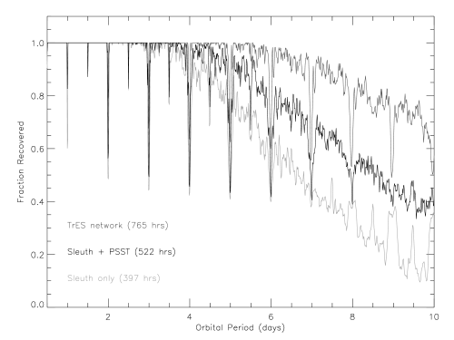
Figure 1.— Transit visibility plot for the Andromeda field calculated from observations made using Sleuth alone (light gray); Sleuth and the PSST (black); and all three TrES telescopes (dark gray). The fraction of transit signals with a given period identifiable from the data is plotted, assuming a requirement of observing 3 distinct transit events, with coverage of at least half of each individual event. About 80% of transit events with periods less than 8 days should be recoverable from the TrES observations, whereas the Sleuth observations alone provide 80% coverage only up to 5 day periods.

Figure 2.— The calculated RMS residual of the binned data versus approximate $V$ magnitude for the stars in our TrES And0 data set. The number of stars with RMS below 1%, 1.5%, and 2% are shown.

Figure 3.— The light curves of the six TrES candidates from the And0 field in Andromeda. The labels denote the source of the light curve. The timeseries have been phased to the best–fit period identified by the box–fitting algorithm of Kovács et al. (2002) using the TrES data, with the exception of T–And0–01241, whose period whose derived from the Sleuth data. The transit event is not present in the data from the other telescopes gathered at the same orbital phase.

Figure 4.— Sample spectra of the And0 TrES candidates obtained with the CfA Digital Speedometers on the FLWO 1.5-m telescope: T–And0–00948 (upper–left) has the low surface gravity of a giant star; T–And0–01241 (upper–right) has the featureless spectrum of an A–type star; T–And0–02022 (center–left) is an evolved F dwarf; T–And0–02462 (center–right) and T–And0–03912 (lower–right) display broadened lines due to the rapid rotation of these stars; T–And0–03874 (lower–left) is an early K–type dwarf.

Figure 5.— The radial velocity orbit of T–And0–02022 as determined from our Digital Speedometer spectra. This system was quickly rejected as a candidate transiting planet after the large radial velocity variation was determined from initial spectroscopic observations. Additional epochs produced a precise orbit, with an eccentricity of $e\sim 0.03$. An initial mass estimate of $0.5\,\mathrm{M}_{\sun}$ was derived for the companion. Future photometry will lead to more precise mass determination for both component stars (see text for a discussion).

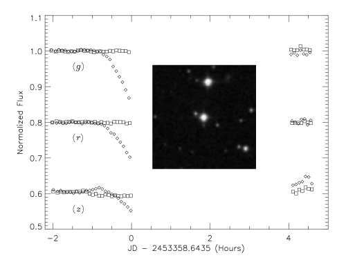
Figure 6.— Follow-up $g$, $r$ and $z$ band photometry with the FLWO 1.2-m telescope of T–And0–03874 (squares) and a neighboring star (diamonds), designated T–And0–02943, that lies $45\arcsec$ away. (The inset $2\arcmin\times 2\arcmin$ Digitized Sky Survey image shows T–And0–03874 at the center and T–And0–02943 to the north.) The flux from each star has been normalized using the out–of–eclipse data, and an offset applied for the purpose of plotting. Inclement weather prevented complete coverage of the predicted eclipse event. Nevertheless, it is evident that T–And0–02943 displays a deep ($>14$%) eclipse, whereas the flux from T–And0–03874 is constant. The observed apparent transits of T–And0–03874 were the result of the blending of the light from these two systems. With a FWHM for T–And0–02943 of $\sim 2.5$ pixels ($\sim 25\arcsec$), some of the light from this star was within the photometric aperture radius ($3$ pixels; $\sim 30\arcsec$) of T–And0–03874.

Figure 7.— TrES photometry of T–And0–03874 and the neighboring eclipsing binary T–And0–02943, phased to the best–fit period (2.6540d) for T–And0–03874 derived by the box–fitting algorithm. Both stars show eclipses with the same orbital period and epoch. The $\sim 1$% transit–like event detected in the light curve of T–And0–03874 was the result of the blending of light from this star and from T–And0–02943, which lies $45\arcsec$ away, comparable to the $30\arcsec$ radius of the TrES PSF.

References

- Alard (2000) Alard, C. 2000, A&AS, 144, 363
- Alonso et al. (2004a) Alonso, R., et al. 2004a, ApJ, 613, L153
- Alonso et al. (2004b) Alonso, R., Deeg, H. J., Brown, T. M., & Belmonte, J. A. 2004b, Astron. Nachr., 325, 594
- Bakos et al. (2004) Bakos, G., Noyes, R. W., Kovács, G., Stanek, K. Z., Sasselov, D. D., & Domsa, I. 2004, PASP, 116, 266
- Bakos et al. (2002) Bakos, G. Á., Lázár, J., Papp, I., Sári, P., & Green, E. M. 2002, PASP, 114, 974
- Bakos et al. (2006) Bakos, G. A., et al. 2006, ApJ, in press (astro-ph/0609369)
- Borucki et al. (2001) Borucki, W. J., Caldwell, D., Koch, D. G., Webster, L. D., Jenkins, J. M., Ninkov, Z., & Showen, R. 2001, PASP, 113, 439
- Bouchy et al. (2005) Bouchy, F., Pont, F., Melo, C., Santos, N. C., Mayor, M., Queloz, D., & Udry, S. 2005, A&A, 431, 1105
- Brown (2003) Brown, T. M. 2003, ApJ, 593, L125
- Charbonneau et al. (2005) Charbonneau, D., et al. 2005, ApJ, 626, 523
- Charbonneau et al. (2006) Charbonneau, D., Brown, T. M., Burrows, A., & Laughlin, G. 2006, in Protostars and Planets V, ed. B. Reipurth, D. Jewitt, & K. Keil (Tucson: Univ. of Arizona Press), in press, (astro-ph/0603376)
- Charbonneau et al. (2004) Charbonneau, D., Brown, T. M., Dunham, E. W., Latham, D. W., Looper, D. L., & Mandushev, G. 2004, in AIP Conf. Proc. 713: The Search for Other Worlds, ed. S. S. Holt & D. Deming (New York: AIP), 151
- Charbonneau et al. (2000) Charbonneau, D., Brown, T. M., Latham, D. W., & Mayor, M. 2000, ApJ, 529, L45
- Charbonneau et al. (2002) Charbonneau, D., Brown, T. M., Noyes, R. W., & Gilliland, R. L. 2002, ApJ, 568, 377
- Charbonneau et al. (2007) Charbonneau, D., Winn, J. N., Everett, M. E., Latham, D. W., Holman, M. J., Esquerdo, G. A., & O’Donovan, F. T. 2007, ApJ, in press (astro-ph/0610589)
- Christian et al. (2006) Christian, D. J., et al. 2006, MNRAS, 372, 1117
- Collier Cameron et al. (2006) Collier Cameron, A., et al. 2006, MNRAS, submitted (astro-ph/0609688)
- Cutri et al. (2003) Cutri, R. M., et al. 2003, 2MASS All Sky Catalog of Point Sources (Amherst: Univ. Massachusetts Press), http://irsa.ipac.caltech.edu/applications/Gator
- Deming et al. (2005a) Deming, D., Brown, T. M., Charbonneau, D., Harrington, J., & Richardson, L. J. 2005a, ApJ, 622, 1149
- Deming et al. (2005b) Deming, D., Seager, S., Richardson, L. J., & Harrington, J. 2005b, Nature, 434, 740
- Drake (2003) Drake, A. J. 2003, ApJ, 589, 1020
- Dravins et al. (1998) Dravins, D., Lindegren, L., Mezey, E., & Young, A. T. 1998, PASP, 110, 610
- Dunham et al. (2004) Dunham, E. W., Mandushev, G. I., Taylor, B. W., & Oetiker, B. 2004, PASP, 116, 1072
- Gaudi (2005) Gaudi, B. S. 2005, ApJ, 628, L73
- Gaudi et al. (2005) Gaudi, B. S., Seager, S., & Mallen-Ornelas, G. 2005, ApJ, 623, 472
- Gaudi & Winn (2007) Gaudi, B. S., & Winn, J. N. 2007, ApJ, 655, 550
- Henry et al. (2000) Henry, G. W., Marcy, G. W., Butler, R. P., & Vogt, S. S. 2000, ApJ, 529, L41
- Hidas et al. (2005) Hidas, M. G., et al. 2005, MNRAS, 360, 703
- Høg et al. (2000a) Høg, E., et al. 2000a, A&A, 357, 367
- Høg et al. (2000b) Høg, E., et al. 2000b, A&A, 355, L27
- Holman et al. (2006) Holman, M. J., et al. 2006, ApJ, 652, 1715
- Holman et al. (2005) Holman, M. J., Winn, J. N., Stanek, K. Z., Torres, G., Sasselov, D. D., Allen, R. L., & Fraser, W. 2005, ApJ, in press (astro-ph/0506569)
- Holt & Deming (2004) Holt, S. S., & Deming, D., ed. 2004, The Search for Other Worlds
- Hut (1981) Hut, P. 1981, A&A, 99, 126
- Kotredes et al. (2004) Kotredes, L., Charbonneau, D., Looper, D. L., & O’Donovan, F. T. 2004, in AIP Conf. Proc. 713: The Search for Other Worlds, ed. S. S. Holt & D. Deming, 173
- Kovács et al. (2002) Kovács, G., Zucker, S., & Mazeh, T. 2002, A&A, 391, 369
- Lasker et al. (1990) Lasker, B. M., Sturch, C. R., McLean, B. J., Russell, J. L., Jenkner, H., & Shara, M. M. 1990, AJ, 99, 2019
- Latham (1992) Latham, D. W. 1992, in ASP Conf. Ser. 32: Complementary Approaches to Double and Multiple Star Research, ed. H. A. McAlister & W. I. Hartkopf, IAU Colloq. 135 (San Fransisco: ASP), 110
- Latham (2003) Latham, D. W. 2003, in ASP Conf. Ser. 294: Scientific Frontiers in Research on Extrasolar Planets, ed. D. Deming & S. Seager (San Fransisco: ASP), 409
- Laughlin et al. (2005) Laughlin, G., Wolf, A., Vanmunster, T., Bodenheimer, P., Fischer, D., Marcy, G., Butler, P., & Vogt, S. 2005, ApJ, 621, 1072
- Mandushev et al. (2005) Mandushev, G., et al. 2005, ApJ, 621, 1061
- McCullough et al. (2005) McCullough, P. R., Stys, J. E., Valenti, J. A., Fleming, S. W., Janes, K. A., & Heasley, J. N. 2005, PASP, 117, 783
- McCullough et al. (2006) McCullough, P. R., et al. 2006, ApJ, 648, 1228
- O’Donovan et al. (2004) O’Donovan, F. T., Charbonneau, D., & Kotredes, L. 2004, in AIP Conf. Proc. 713: The Search for Other Worlds, ed. S. S. Holt & D. Deming, 169
- O’Donovan et al. (2006a) O’Donovan, F. T., et al. 2006a, ApJ, 651, L61
- O’Donovan et al. (2006b) O’Donovan, F. T., et al. 2006b, ApJ, 644, 1237
- Pepper et al. (2004) Pepper, J., Gould, A., & Depoy, D. L. 2004, in AIP Conf. Proc. 713: The Search for Other Worlds, ed. S. S. Holt & D. Deming, 185
- Pont et al. (2005) Pont, F., Bouchy, F., Melo, C., Santos, N. C., Mayor, M., Queloz, D., & Udry, S. 2005, A&A, 438, 1123
- Pont et al. (2006) Pont, F., Zucker, S., & Queloz, D. 2006, MNRAS, 373, 231
- Rauer et al. (2004) Rauer, H., Eislöffel, J., Erikson, A., Guenther, E., Hatzes, A. P., Michaelis, H., & Voss, H. 2004, PASP, 116, 38
- Seager & Mallén-Ornelas (2003) Seager, S., & Mallén-Ornelas, G. 2003, ApJ, 585, 1038
- Sirko & Paczyński (2003) Sirko, E., & Paczyński, B. 2003, ApJ, 592, 1217
- Smith et al. (2006) Smith, A. M. S., et al. 2006, MNRAS, 373, 1151
- Street et al. (2003) Street, R. A., et al. 2003, in ASP Conf. Ser. 294: Scientific Frontiers in Research on Extrasolar Planets, ed. D. Deming & S. Seager, 405
- Szentgyorgyi et al. (2005) Szentgyorgyi, A. H., et al. 2005, American Astronomical Society Meeting Abstracts, 207, 110.10
- Tingley (2004) Tingley, B. 2004, A&A, 425, 1125
- Tody (1993) Tody, D. 1993, in ASP Conf. Ser. 52: Astronomical Data Analysis Software and Systems II, ed. R. J. Hanisch, R. J. V. Brissenden, & J. Barnes (San Fransisco: ASP), 173
- Torres et al. (2004) Torres, G., Konacki, M., Sasselov, D. D., & Jha, S. 2004, ApJ, 614, 979
- Udalski et al. (2002) Udalski, A., et al. 2002, Acta Astron., 52, 1
- Vidal-Madjar et al. (2003) Vidal-Madjar, A., Lecavelier des Etangs, A., Désert, J.-M., Ballester, G. E., Ferlet, R., Hébrard, G., & Mayor, M. 2003, Nature, 422, 143
- Young (1967) Young, A. T. 1967, AJ, 72, 747
- Zacharias et al. (2004) Zacharias, N., Urban, S. E., Zacharias, M. I., Wycoff, G. L., Hall, D. M., Monet, D. G., & Rafferty, T. J. 2004, AJ, 127, 3043