The Large Scale Structure of $f(R)$ Gravity

Abstract

We study the evolution of linear cosmological perturbations in $f(R)$ models of accelerated expansion in the physical frame where the gravitational dynamics are fourth order and the matter is minimally coupled. These models predict a rich and testable set of linear phenomena. For each expansion history, fixed empirically by cosmological distance measures, there exists two branches of $f(R)$ solutions that are parameterized by $B\propto d^{2}f/dR^{2}$. For $B<0$, which include most of the models previously considered, there is a short-timescale instability at high curvature that spoils agreement with high redshift cosmological observables. For the stable $B>0$ branch, $f(R)$ models can reduce the large-angle CMB anisotropy, alter the shape of the linear matter power spectrum, and qualitatively change the correlations between the CMB and galaxy surveys. All of these phenomena are accessible with current and future data and provide stringent tests of general relativity on cosmological scales.

I Introduction

Cosmic acceleration can be explained either by missing energy with an exotic equation of state, dubbed dark energy, or by a modification of gravity on large scales. Indeed the cosmological constant can be considered either as a constant added to the Einstein-Hilbert action or as vacuum energy. Non-trivial modifications where the addition is a non-linear function $f(R)$ of the Ricci scalar that becomes important only at the cosmologically low values of $R$ have also been shown to cause acceleration Carroll et al. (2004); Capozziello et al. (2003); Nojiri and Odintsov (2003). They are furthermore free of ghosts and other types of instabilities for a wide range of interesting cases Nojiri and Odintsov (2003); Dick (2004); De Felice et al. (2006).

Solar-system tests of gravity provide what is perhaps the leading challenge to $f(R)$ models as a complete theory of gravity Chiba (2003). The equivalence of $f(R)$ models to scalar-tensor theories lead to conflicts with parameterized post-Newtonian constraints at a background cosmological density of matter. It is however still controversial whether the whole class of $f(R)$ modifications can be ruled out by this equivalence. Matter in the solar system becomes non-minimally coupled in the transformed frame leading to non-trivial modifications of the scalar field potential. In the original Jordan—or physical—frame, it has been shown that the Schwarzschild metric solves the modified Einstein equations of a wide range of $f(R)$ models Brevik et al. (2004); Multamaki and Vilja (2006a) but this solution is not necessarily relevant for the solar system Erickcek et al. (2006). Recent work has also raised the question as to whether solar-system gravity problems may become tractable if $f(R)$ is viewed as simply a first-order correction term to the high $R$ limit of general relativity Cembranos (2006); Sotiriou (2006); Shao et al. (2006); Faraoni (2006).

Regardless of the outcome of small-scale tests of gravity in $f(R)$ models, it is worthwhile to examine the cosmological consequences of treating $f(R)$ as an effective theory valid for a cosmologically appropriate range of curvatures. At the very least by making concrete predictions of cosmological phenomena in these models, one gains insight on how cosmology can test gravity at the largest scales.

In this Paper, we develop linear perturbation theory for predicting cosmological observables such as the Cosmic Microwave Background (CMB) and the large-scale structure of the universe exhibited in galaxy surveys. We work in the physical frame where the matter is minimally coupled and obeys simple conservation laws.

We begin in §II by reviewing the properties of $f(R)$ models and their relationship to the expansion history of the universe. In §III, we derive the fourth order perturbation equations and, using general properties demanded by energy-momentum conservation Bardeen (1980); Hu and Eisenstein (1999); Bertschinger (2006), recast them into a tractable second order form. In §IV we identify a short time scale instability that renders a wide class of $f(R)$ models not viable cosmologically. We present solutions on the stable branch in §V and explore their impact on cosmological power spectra in §VI. We discuss these results in §VII.

II Expansion History

We consider a modification to the Einstein-Hilbert action of the form Starobinsky (1980)

$$S=\int d^{4}x\sqrt{-g}\left[{R+f(R)\over 2\mu^{2}}+{\cal L}_{\rm m}\right]\,,$$ (1)

where $R$ is the Ricci scalar, which we will sometimes refer to as the curvature, $\mu^{2}\equiv 8\pi G$, and ${\cal L}_{m}$ is the matter Lagrangian. Variation with respect to the metric yields the modified Einstein equations

$$G_{\alpha\beta}+f_{R}R_{\alpha\beta}-({f\over 2}-\Box f_{R})g_{\alpha\beta}-\nabla_{\alpha}\nabla_{\beta}f_{R}=\mu^{2}T_{\alpha\beta}\,,$$ (2)

where $f_{R}\equiv df/dR$ and likewise $f_{RR}\equiv d^{2}f/dR^{2}$ below. We define the metric to include scalar linear perturbations around a flat FRW background in the Newtonian or longitudinal gauge

$$ds^{2}=-(1+2\Psi)dt^{2}+a^{2}(1+2\Phi)dx^{2}\,.$$ (3)

Given that the expansion history and dynamics of linear perturbations are well-tested in the high curvature, high redshift limit by the CMB, we restrict our considerations to models that satisfy Carroll et al. (2004); Capozziello et al. (2003); Nojiri and Odintsov (2003)

$$\lim_{R\rightarrow\infty}f(R)/R\rightarrow 0\,.$$ (4)

With this restriction, the main modifications for viable models with stable high curvature limits arise well after the radiation becomes a negligible contributor to the stress energy tensor. We can then take it to have the matter-dominated form

$$T^{0}_{\hphantom{0}0} = -\rho(1+\delta)\,,$$

$$T^{0}_{\hphantom{0}i} = \rho\partial_{i}q\,,$$

$$T^{i}_{\hphantom{i}j} = 0\,.$$ (5)

The modified Einstein equations with the FRW background metric and $\delta=q=0$ yields the modified Friedmann equation

$$H^{2}-f_{R}(HH^{\prime}+H^{2})+{1\over 6}f+H^{2}f_{RR}R^{\prime}={\mu^{2}\rho\over 3}\,.$$ (6)

Here and throughout, primes denote derivatives with respect to $\ln a$.

There is sufficient freedom in the function $f(R)$ to reproduce any desired expansion history $H$. Hence the expansion history alone cannot be used as a test of general relativity though it can rule out specific forms of $f(R)$. The dynamics of linear perturbations on the other hand do test general relativity as we shall see.

We therefore seek to determine a family of $f(R)$ functions that is consistent with a given expansion history Multamaki and Vilja (2006b); Capozziello et al. (2006); Nojiri and Odintsov (2006a); Nojiri and Odintsov (2006b); de la Cruz-Dombriz and Dobado (2006). Without loss of generality, we can parameterize the expansion history in terms of an equivalent dark energy model

$$H^{2}={\mu^{2}\over 3}(\rho+\rho_{\rm DE})\,.$$ (7)

This yields a second order differential equation for $f(R)$

$$-f_{R}(HH^{\prime}+H^{2})+{1\over 6}f+H^{2}f_{RR}R^{\prime}=-{\mu^{2}\rho_{\rm DE}\over 3}\,,$$ (8)

where $H^{2}$ and $R$ are fixed functions of $\ln a$ given the matching to the dark energy model.

For convenience, let us define the dimensionless quantities

$$E={H^{2}\over H_{0}^{2}}\,,\quad{R\over H_{0}^{2}}=3(4E+E^{\prime})\,,\quad y={f\over H_{0}^{2}}\,.$$ (9)

Here $H_{0}\equiv H(\ln a=0)=h/2997.9$ Mpc^-1 is the Hubble constant. The modified Friedmann equation can be recast into an inhomogeneous differential equation for $y(\ln a)$

$$L[y] = -{\mu^{2}}{\rho_{\rm DE}\over H_{0}^{2}}\left({4E^{\prime}+E^{\prime\prime}\over E}\right)\,,$$ (10)

where the differential operator on the lhs is given by

$$L[y] \equiv y^{\prime\prime}-\left(1+{1\over 2}{E^{\prime}\over E}+{4E^{\prime\prime}+E^{\prime\prime\prime}\over 4E^{\prime}+E^{\prime\prime}}\right)y^{\prime}$$ (11)

$$+{1\over 2}\left({4E^{\prime}+E^{\prime\prime}\over E}\right)y\,.$$

For illustrative purposes, we take an expansion history that matches a dark energy model with a constant equation of state $w$,

$$E=(1-\Omega_{\rm DE})a^{-3}+\Omega_{\rm DE}a^{-3(1+w)}\,,$$ (12)

and

$${\mu^{2}\over 3}{\rho_{\rm DE}\over H_{0}^{2}}=\Omega_{\rm DE}a^{-3(1+w)}\,.$$ (13)

Since Eq. (11) is a second-order differential equation, the expansion history does not uniquely specify $f(R)$ but instead allows a family of solutions that are distinguished by initial conditions. This additional freedom reflects the fourth-order nature of $f(R)$ gravity.

To set the initial conditions, take $y_{\pm}$ to be the two solutions of the homogeneous equation $L[y]=0$. At high curvature, these solutions are power laws $y_{\pm}\propto a^{p_{\pm}}$ with

$$p_{\pm}={-7\pm\sqrt{73}\over 4}\,.$$ (14)

Since $p_{-}\approx-3.9$, stimulation of this decaying mode violates the condition that $f_{R}/R\rightarrow 0$ at high $R$. We therefore set its amplitude to zero in our solutions (c.f. Capozziello et al. (2006); Amendola et al. (2006a, b)). The particular solution in the high curvature limit becomes

$$y_{\rm part} = {6\Omega_{\rm DE}\over 6w^{2}+5w-2}a^{-3(1+w)}\,.$$ (15)

Therefore when numerically integrating Eq. (11) we take

$$y(\ln a_{i}) = Ay_{+}(\ln a_{i})+y_{\rm part}(\ln a_{i})\,,$$ (16)

$$y^{\prime}(\ln a_{i}) = p_{+}Ay_{+}(\ln a_{i})-3(1+w)y_{\rm part}(\ln a_{i})\,,$$

at some initial epoch $a_{i}\sim 10^{-2}$.

Since the modifications to gravity appear at low redshifts, it is more convenient to parameterize the individual solutions in the family by the final conditions rather than the growing mode amplitude of the initial conditions. Given that a constant $f(R)$ is simply a cosmological constant and a linear one represents a rescaling of $G$ or $\mu$, it is $f_{RR}$, the second derivative, that controls phenomena that are unique to the modification. In particular, we shall see that a specific dimensionless quantity

$$B = {f_{RR}\over 1+f_{R}}{R^{\prime}}{H\over H^{\prime}}$$

$$= {2\over 3(1+f_{R})}{1\over 4E^{\prime}+E^{\prime\prime}}{E\over E^{\prime}}\left(y^{\prime\prime}-y^{\prime}{4E^{\prime\prime}+E^{\prime\prime\prime}\over 4E^{\prime}+E^{\prime\prime}}\right)\,,$$

is most closely linked with the phenomenology. $B$ is a strongly growing function in our solutions and in the high curvature limit has a growth rate

$$p_{B}\equiv{B^{\prime}\over B}$$ (18)

given by $p_{B}=3+p_{+}$, if the growing mode dominates, and $p_{B}=-3w$, if the particular mode dominates.

We will therefore characterize solutions with a given expansion history family by $B_{0}\equiv B(\ln a=0)$. If $B_{0}=0$ and the background expansion is given by $w=-1$ then $f(R)=$ const., $B(\ln a)=0$ and the model has a true cosmological constant. More generally $B=0$ will correspond in linear theory to the dynamics of a dark energy component for scales above the dark energy sound horizon.

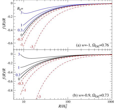
In Fig. 1, we plot the family of $f(R)$ models that match two representative expansion histories parameterized by $(w,\Omega_{\rm DE},h)$. These models are chosen to be consistent with current WMAP CMB data Spergel et al. (2006) and span a range that is consistent with supernovae acceleration measures. Given the similarity between these models, we will take the $w=-1$ $\Lambda$CDM expansion history for illustrative purposes below.

The linear perturbation analysis that follows does not require the matching to the specific expansion histories parameterized by $(w,\Omega_{\rm DE},h)$ here. This reverse engineering is only a device to find observationally acceptable $f(R)$ models. What is required is that the background solutions provide $H(\ln a)$ and $B(\ln a)$. On the other hand, linear perturbation theory does inform the choice of a background solution. We shall find in §IV that the $B<0$ branch of the family is unstable to linear perturbations in the high curvature regime.

Figure 1: Every expansion history that can be parameterized by a dark energy model with $\rho_{\rm DE}(\ln a)$ can be reproduced by a one parameter family of $f(R)$ models, indexed by $B_{0}\propto f_{RR}/(1+f_{R})$ at the present epoch (left end point of curves), that approaches the Einstein-Hilbert action in the high curvature limit. (a) $\Lambda$CDM expansion history ($w=-1$, $\Omega_{\rm DE}=0.76$, $h=0.73$). (b) Dynamical dark energy expansion history ($w=-0.9$, $\Omega_{\rm DE}=0.73$, $h=0.69$).

III Linear Perturbation Equations

The modified Einstein equations (2) represent a fourth-order set of differential equations for the two metric perturbations $\Psi$ and $\Phi$ in the presence of matter density and momentum fluctuations $\delta$ and $q$. To solve this system of equations, we introduce auxiliary parameters to recast it as a larger set of second-order differential equations. It is numerically and pedagogically advantageous to choose these auxiliary parameters so that their effect vanishes at large scales and early times.

On superhorizon scales ($k/aH\ll 1$), the evolution of metric perturbations must be consistent with the background evolution provided that the background solution is valid, i.e. that fluctuations about it are stable. Bertschinger Bertschinger (2006) showed that the familiar conservation of the curvature fluctuation on comoving hypersurfaces ($\zeta^{\prime}=0$) for adiabatic fluctuations in a flat universe applies to any metric based modified gravity model that obeys energy momentum conservation $\nabla^{\mu}T_{\mu\nu}=0$. The gauge transformation into the Newtonian gauge

$$\zeta=\Phi+Hq$$ (19)

implies

$$\zeta^{\prime}=\Phi^{\prime}+H^{\prime}q+Hq^{\prime}=0\,,\,\,\,(k=0)\,,$$ (20)

and momentum conservation requires

$$Hq^{\prime}=-\Psi$$ (21)

so that

$$\Phi^{\prime}-\Psi+H^{\prime}q=0\,,\,\,\,(k=0)\,.$$ (22)

Combining Eq. (21) and (22) yields a second order differential equation for the Newtonian metric perturbations Hu and Eisenstein (1999)

$$\Phi^{\prime\prime}-\Psi^{\prime}-{H^{\prime\prime}\over H^{\prime}}\Phi^{\prime}-\left({H^{\prime}\over H}-{H^{\prime\prime}\over H^{\prime}}\right)\Psi=0\,,\,\,\,(k=0)\,.$$ (23)

The evolution of the metric fluctuations must in this way be consistent with the expansion history defined by $H$. Note that this equation applies to any modified gravitational scenario that satisfies the required conditions. The DGP braneworld acceleration model Dvali et al. (2000) represents another valid application Sawicki et al. (2006). What does require a specification of a theory is the relation between $\Phi$ and $\Psi$. Under general relativity and assuming $T_{\mu\nu}$ takes the matter-only form of Eq. (5), the closure relation is $\Phi=-\Psi$ and Eq. (23) in fact applies on all scales. With a dynamical dark energy component in $T_{\mu\nu}$, it applies above the dark energy sound horizon Hu (1998).

To capture the metric evolution of $f(R)$ models for $k\neq 0$, let us introduce two parameters: $\theta$ the deviation from $\zeta$ conservation, Eq. (22)

$$\zeta^{\prime}=\Phi^{\prime}-\Psi+H^{\prime}q = {H^{\prime}\over H}\left({k\over aH}\right)^{2}B\theta\,,$$ (24)

and $\epsilon$ the deviation from the superhorizon metric evolution Eq. (23)

$$\Phi^{\prime\prime}-\Psi^{\prime}-{H^{\prime\prime}\over H^{\prime}}\Phi^{\prime}-\left({H^{\prime}\over H}-{H^{\prime\prime}\over H^{\prime}}\right)\Psi$$

$$\qquad=\left({k\over aH}\right)^{2}B\epsilon\,.$$ (25)

The coefficients in front of the deviation parameters are chosen to bring out the fact that their effect vanishes as $k/aH\rightarrow 0$ and $B\rightarrow 0$ so long as the dynamics guarantees stable behavior of the parameters themselves (see §IV).

The Einstein equations can then be recast as a second order differential equation for $\epsilon$ and constraint equations for the other metric variables. Since $\epsilon$ itself contains second derivatives of the fundamental metric perturbations $\Phi$ and $\Psi$, the equations are implicitly fourth order. It will be convenient to separate out two linear combinations of the underlying metric fluctuation

$$\Phi_{-}={1\over 2}(\Phi-\Psi)\,,\quad S=2\Phi+\Psi\,,$$ (26)

and a reduced mass scale or rescaling of $G$

$$\tilde{\mu}^{2}(\ln a)={\mu^{2}\over 1+f_{R}(\ln a)}\,.$$ (27)

In terms of these variables, the $0i$ component of the Einstein equations becomes a dynamical equation for $\epsilon$

$$B(\epsilon^{\prime}+G_{1}\epsilon) = {1\over 3}G_{2}S-{1\over 3}(S-2\Phi_{-})+{B\over 6}{E^{\prime}\over E}(S-2\Phi_{-})$$

$$+\left({1\over 2}{E^{\prime}\over E}+{1\over 3}{\tilde{\mu}^{2}\rho\over H^{2}}\right)Hq$$

$$+\left[{\tilde{\mu}^{2}\rho\over H^{2}}\left(4+{E^{\prime\prime}\over E^{\prime}}\right)-{1\over 2}{E^{\prime}\over E}\left({k\over aH}\right)^{2}\right]\theta\,,$$

where

$$G_{1} = 1-{E^{\prime}\over E}+2{E^{\prime\prime}\over E^{\prime}}-{4E^{\prime\prime}+E^{\prime\prime\prime}\over 4E^{\prime}+E^{\prime\prime}}+{1\over 2}{E^{\prime}\over E}B+2{B^{\prime}\over B}\,,$$

$$G_{2} = 4+{E^{\prime\prime}\over E^{\prime}}+{B^{\prime}\over B}-G_{1}\,.$$ (29)

The metric fluctuations $S$ and $\Phi_{-}$ act as sources to $\epsilon$ which then feed back into their evolution weighted by $(Bk/aH)^{2}$. To complete this system, the dynamics of $\theta$ are supplied by the derivative of its definition Eq. (24) combined with Eq. (25)

$$\theta^{\prime}+\left(-2-{3\over 2}{E^{\prime}\over E}+{B^{\prime}\over B}\right)\theta = 2{E\over E^{\prime}}\epsilon\,.$$ (30)

Eqs. (III) and (30) can also be combined to eliminate $\theta$ leaving a second-order differential equation for $\epsilon$. This combined relation may alternately be derived directly from the trace of the $ij$ component of the Einstein equations.

As in general relativity, the remaining Einstein equations become constraint equations given the dynamical variables $\Delta,Hq,\epsilon,\theta$. The $00$ equation may be expressed as the modified Poisson equation,

$$2\Phi_{-}-{B\over 2}{E^{\prime}\over E}{E^{\prime}\over 4E^{\prime}+E^{\prime\prime}}(S+3B\epsilon)={\tilde{\mu}^{2}a^{2}\rho\over k^{2}}\Delta\,,$$ (31)

where $\Delta$ is the density perturbation in the comoving gauge

$$\Delta=\delta-3Hq\,,$$ (32)

and the trace-free $ij$ component becomes

$$\Phi+\Psi = {2\over 3}(S-\Phi_{-})$$

$$= {B\over 2}{E^{\prime}\over E}(Hq)-B\left({k\over aH}\right)^{2}$$

$$\times\Big{[}{1\over 3}{E^{\prime}\over 4E^{\prime}+E^{\prime\prime}}(S+3B\epsilon)+{1\over 2}{E^{\prime}\over E}B\theta\Big{]}\,.$$

Note that as $B\rightarrow 0$ and $\tilde{\mu}\rightarrow\mu$ these constraint equations become the usual Poisson and anisotropy equations. In particular for $B=0$, the dark energy-closure relation $\Phi=-\Psi$ is recovered.

Finally, the conservation laws provide the dynamics for the matter fluctuations and are unmodified by $f(R)$

$$\Delta^{\prime}=\left(\frac{k}{aH}\right)^{2}Hq-3\zeta^{\prime}\,,$$ (34)

$$Hq^{\prime}=-\Psi=-\frac{1}{3}(S-4\Phi_{-}).$$ (35)

The impact of the modification to gravity comes from the metric evolution. Eq. (24) implies

$$\zeta^{\prime}={H^{\prime}\over H}\left({k\over aH}\right)^{2}B\theta\,.$$ (36)

In fact directly integrating Eq. (36) and checking for consistency between $Hq$ defined through Eq. (19) and Eq. (35) tests the numerical accuracy of solutions.

Along with initial conditions for each of the fluctuations, these equations provide a complete and exact description of scalar linear perturbation theory in $f(R)$ gravity for a matter-only universe.

IV Stability at High Curvature

The fourth-order nature of the linear perturbation equations derived in the previous section raises the question of stability in the high-curvature limit to general relativity Dolgov and Kawasaki (2003); Zhang (2006); Woodard (2006); Siefert and Wald (2007). Strongly unstable metric fluctuations can create order unity effects that invalidate the background expansion history.

The key equations for stability are (III) and (30) which describe the evolution of the deviation parameters. Consider the high redshift limit of high curvature where $|B|\rightarrow 0$ and wavelengths of interest are well outside the horizon $k/aH\ll 1$. In this limit the evolution equations simplify to

$$\epsilon^{\prime\prime}+\left({7\over 2}+4p_{B}\right)\epsilon^{\prime}+{2\over B}\epsilon={1\over B}F(\Phi_{-},S,Hq)\,,$$ (37)

where $F(\Phi_{-},S,Hq)$ is the source function for the deviation $\epsilon$ and recall $p_{B}$ is the growth index of $B$ from Eq. (18). The details of $F$ are not important for the stability analysis other than that it provides a source that is of order the perturbation parameters that are its arguments. Under the assumption that the general relativistic solution is stably recovered in this limit, it acts as an external source to the deviations. The stability question can be phrased as whether $\epsilon$ remains self-consistently of order these sources or grows and prevents the recovery of the solutions.

The stability equation (37) has the peculiar feature that the frequency squared $2/B$ diverges as $|B|\rightarrow 0$ independently of $k$, resembling a divergent real or imaginary mass term. Evolution of $\epsilon$ can occur on a time scale much shorter than the expansion time. If $B<0$, $\epsilon$ is highly unstable and deviations will grow exponentially. If $B>0$, $\epsilon$ is highly stable and is driven to the value required by the source function $\epsilon=F/2$. This short time scale behavior can also be seen directly in the 4th order form of the Einstein equation. The trace of the $ij$ equation or the derivative of the $0i$ equation have their 4th order terms multiplied by the small parameter $B$.

Thus despite the apparent recovery of general relativity in the action at high curvature $R$, the general-relativistic solutions to linear perturbation theory are not recovered for $B<0$. In terms of $f(R)$, $B\propto f_{RR}$ in this limit and hence models like Carroll et al. (2004)

$$f(R)=-{M^{2+2n}\over R^{n}}\,,\quad(n>0)\,,$$ (38)

and Zhang (2006)

$$f(R)=-M^{2}\exp(-R/\lambda M^{2})\,,$$ (39)

are included in this class of unstable models.

The instability causes any finite patch of a universe that starts at high curvature to break away from the background solution into either a low curvature solution or a singularity. The low curvature $R\ll G\rho$ solutions on the other hand are stable and in fact correspond to the background expansion histories studied by Amendola et al. (2006a); Bean et al. (2006). However these expansion histories have gravity modified throughout the matter dominated epoch and in particular $a\propto t^{1/2}$. They produce phenomenology at high redshift that would violate constraints from the CMB. We will omit them from further consideration below.

V Metric Evolution Solutions

In this section we discuss the numerical solutions of the linear perturbation equations on the stable $B>0$ branch. To expose the underlying features of the solutions, we examine the relevant limiting cases below. We begin with the initial epoch where $|B|\ll 1$ and the fluctuations are superhorizon sized $k/aH\ll 1$. We then examine large scale or “superhorizon” modes where $B^{1/2}k/aH\ll 1$ whose evolution is completely determined by the background expansion history and the form of $f(R)$. Finally we track the evolution of small scale or “subhorizon” modes until $B^{1/2}k/aH\gg 1$ where their evolution reaches the simple form implied by quasistatic equilibrium.

V.1 Initial Conditions

On the stable $B>0$ branch, we can set the initial conditions when $B\ll 1$ and the mode is superhorizon sized, $k/aH\ll 1$. In this case, the initial conditions for the normal fluctuation parameters follow the general-relativistic expectation

$$\Phi_{i} = {3\over 5}\zeta_{i}\,,$$

$$\Psi_{i} = -\Phi_{i}\,,$$

$$\Delta_{i} = {2\over 3}\left({k\over aH}\right)^{2}\Phi_{i}\,,$$

$$Hq_{i} = {2\over 3}\Phi_{i}\,,$$ (40)

where $\zeta_{i}$=const. is the initial comoving curvature. These relations also imply $\Phi_{-}=\Phi$ and $S=\Phi$ with vanishing first derivatives initially.

Detailed balance gives the deviation parameters as

$$\theta_{i} = {1\over 9}p_{B}\Phi_{i}\,,$$

$$\epsilon_{i} = -{3\over 2}\left({5\over 2}+p_{B}\right)\theta_{i}\,,$$ (41)

and the high frequency term in their evolution equations ensures that they stay locked to these relations until $B$ becomes non-negligible.

V.2 Superhorizon Evolution

Given that $\theta$ and $\epsilon$ are locked to the initial values of Eq. (41) when $B\ll 1$, their definitions in Eq. (24), (25) imply that they have negligible effect on the evolution of the metric fluctuations $\Phi$, $\Psi$. This remains true even as the mode evolves into the $B\sim 1$ regime if $k/aH\ll 1$. In particular, the anisotropy relation of Eq. (III) becomes

$$\Phi+\Psi=BH^{\prime}q$$ (42)

and closes the general relation for superhorizon metric fluctuations Eq. (23):

$$\Phi^{\prime\prime}+\left(1-{H^{\prime\prime}\over H^{\prime}}+{B^{\prime}\over 1-B}+B{H^{\prime}\over H}\right)\Phi^{\prime}$$ (43)

$$\qquad+\left({H^{\prime}\over H}-{H^{\prime\prime}\over H^{\prime}}+{B^{\prime}\over 1-B}\right)\Phi=0\,,\,\,\,(k=0)\,.$$

The evolution of $\Phi$ is completely determined by the background evolution and the specification of $f(R)$. Formally, this solution also applies to the unstable branch $B<0$ at $k=0$ but is only valid at finite $k$ for large $|B|$. The point at which $B=1$ is a regular singular point for typical $B(\ln a)$ and so $\Phi$ evolves smoothly through it. $\Phi$ will grow on the expansion time scale if

$${H^{\prime}\over H}-{H^{\prime\prime}\over H^{\prime}}+{B^{\prime}\over 1-B}<0\,.$$ (44)

Growth is typically a transient phenomenon at the onset of acceleration given that the presence of matter makes $H^{\prime}/H-H^{\prime\prime}/H^{\prime}$ positive. For example, if the expansion rate approaches the de Sitter case of a constant in the future $H^{\prime}/H\rightarrow 0$ and the solution to Eq. (V.2) becomes

$$\Phi={C_{1}\over a}+{C_{2}\over a}\int da{(1-B)H^{\prime}}\,,\,\,\,(H^{\prime}/H\rightarrow 0)\,,$$ (45)

where $C_{1}$ and $C_{2}$ are constants. This implies decaying solutions unless $BH^{\prime}$ grows. $H^{\prime}$ decays and, since in de Sitter $R\rightarrow$ const, $B$ should asymptote to a constant. Eq. (45) then implies $\Phi\propto 1/a$. Note that this stability analysis differs from treatments that take a pure de Sitter expansion with no matter since that assumption forces a closure relation of $\Phi=\Psi$ (c.f. Faraoni (2005a, b)).

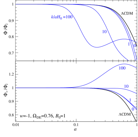
An example of the superhorizon evolution of the metric is shown in Fig. 2 ($k=0$ curves) for a model with $B_{0}=1$. While $\Phi$ is monotonically smaller than the $B=0$ $\Lambda$CDM prediction, $\Phi_{-}$ is monotonically larger due to the closure relation between $\Phi$ and $\Psi$ of Eq. (42).

Figure 2: Evolution of metric fluctuations $\Phi$ (upper panel) and $\Phi_{-}$ (lower panel) for $B_{0}=1$ and a $\Lambda$CDM expansion history. The different closure relations on super and sub-horizon scales for $\Psi$, Eqs. (42) and (46), lead to qualitatively different evolution for the two limits with a transition region in between. $\Phi_{-}$, which controls effects in the CMB and enters directly into the Poisson equation, has a scale-dependent growth that makes it increasingly larger than the $\Lambda$CDM prediction at high $k$. Results for other values of $B_{0}$ can be scaled from this figure by noting that the transition occurs when $k/aH\approx B^{-1/2}$.

V.3 Subhorizon Evolution

For subhorizon scales where $k/aH\gg 1$, Eqs. (III) and (30) form an oscillator equation whose frequency scales as $k/aH$. Therefore the amplitude of $\epsilon$ is driven to zero when compared with $\Phi_{-}$. When combined with the Poisson and anisotropy equation, this requires Zhang (2006)

$$\lim_{Bk/aH\rightarrow\infty}S\rightarrow 0\,,\quad\Psi\rightarrow-2\Phi\,,\quad\Phi_{-}\rightarrow{3\over 2}\Phi$$ (46)

The Poisson equation then takes the simple form

$$k^{2}\Phi_{-}={1\over 2}{\tilde{\mu}^{2}a^{2}\rho}\Delta$$ (47)

and the conservation laws become

$$\Delta^{\prime} = \left({k\over aH}\right)^{2}Hq\,,$$

$$Hq^{\prime} = {4\over 3}\Phi_{-}\,,$$ (48)

where we have dropped temporal derivatives when compared with spatial gradients where appropriate. This system describes a scale free evolution for $\Phi_{-}$ or $\Delta$. The transition between these two scale-free regimes occurs when $(k/aH)\sim B^{-1/2}$. This scale- and time-dependent transition leads to a scale-dependent growth rate. Unlike for $\Phi$, $\Phi_{-}$ has monotonically enhanced power as $k$ increases on the $B>0$ branch. Because of the time dependence of the transition, the total growth to $z=0$ continues to increase with $k$ even for $k/aH\gg B^{-1/2}$.

In Fig. 2, we show the full numerical solution from the initial conditions through the super- to the sub-horizon evolution for a few representative modes.

VI Power-Spectra Observables

The scale dependences of the linear growth rate of metric and density perturbations change predictions for cosmological power spectra in the linear regime. Let us make the usual assumption that the initial spectrum of fluctuations in the comoving curvature is given by a power law. For a starting epoch during matter domination, this power law is modified by the usual matter-radiation transfer function $T(k)$

$${k^{3}P_{\zeta_{i}}\over 2\pi^{2}}=\delta_{\zeta}^{2}\left({k\over k_{\rm n}}\right)^{n-1}T^{2}(k)\,,$$ (49)

where $\delta_{\zeta}$ is the rms amplitude at the normalization scale $k_{\rm n}$.

The modifications to the CMB depend on the scale-dependent change in the potential growth rate

$$G(a,k)={\Phi_{-}(a,k)\over\Phi_{-}(a_{i},k)}\,,$$ (50)

through the Integrated Sachs-Wolfe (ISW) effect. This effect comes from the differential redshift that CMB photons suffer as they transit the evolving potential. It contributes to the angular power spectrum of temperature anisotropies as

$$C^{\rm II}_{l}=4\pi\int\frac{{d}k}{k}[I^{\rm I}_{l}(k)]^{2}{9\over 25}{k^{3}P_{\zeta_{i}}\over 2\pi^{2}}\,,$$ (51)

where

$$I^{\rm I}_{l}(k)=2\int dz{dG\over dz}j_{l}(kD)\,.$$ (52)

Here $D=\int dz/H$ is the comoving distance out to redshift $z$.

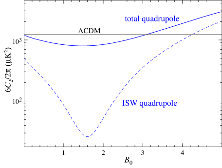
In Fig. 3, we show the quadrupole power as a function of $B_{0}$ contributed by the ISW effect as well as the total quadrupole. Power in the quadrupole arises near scales of $k/H_{0}\sim 10$ and so the weak evolution of $\Phi_{-}$ shown in Fig. 2 reduces it near $B_{0}\sim 1$. In fact there is a minimum around $B_{0}\approx 3/2$, where the ISW effect is a negligible contributor to the power, and a substantial reduction for $0.2\lesssim B_{0}\lesssim 2.5$. Further reduction of large-scale power can be achieved by changing the initial power spectrum to simultaneously suppress horizon scale power in the Sachs-Wolfe effect from recombination. Hence these models provide the opportunity to bring the predicted ensemble-averaged quadrupole closer to the measurements on our sky Spergel et al. (2006). Models with $B_{0}\gtrsim 3$ produce an excess of large-angle anisotropy and exacerbate the tension with the data. Note however that due to sample variance, changes in the likelihood will be small. We will address constraints on the models in a separate work.

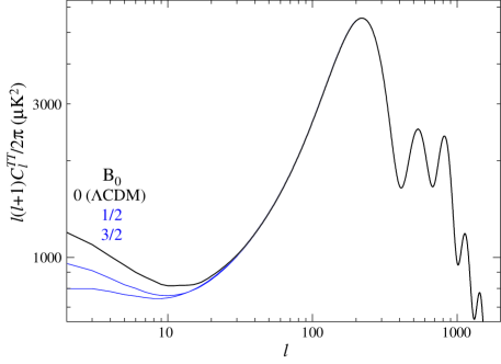
We show the full spectrum of temperature anisotropy $C_{l}^{TT}$ in Fig. 4 for a few representative values of $B_{0}$. Given that the changes to the power spectrum occur mainly at the lowest multipoles, WMAP constraints on the amplitude of the peaks can be directly translated into a normalization of the power spectrum on scales corresponding to the acoustic peaks. For the $\Lambda$CDM expansion history of $w=-1$, $\Omega_{\rm DE}=1-\Omega_{m}=0.76$, $h=0.73$ the normalization from WMAP is $\delta_{\zeta}=4.52\times 10^{-5}$ for an optical depth to reionization of $\tau=0.092$. We further take a tilt of $n=0.958$, $\Omega_{b}h^{2}=0.0223$.

Figure 3: CMB quadrupole power $6C_{2}/2\pi$ contributed by the modified ISW effect (dashed curve) and total (solid curve) as a function of $B_{0}$ in the $\Lambda$CDM expansion history. For reference, the $\Lambda$CDM total quadrupole is also shown (horizontal line). The change in the growth of the potential causes a near nulling of the ISW effect at $B_{0}\approx 3/2$ and a substantial reduction of power between $0.2\lesssim B_{0}\lesssim 2.5$.

Figure 4: CMB angular power spectra for the $\Lambda$CDM expansion history for $B_{0}=0$ ($\Lambda$CDM), 1/2, 3/2. Power in the low multipoles is lowered by the reduction in the ISW effect. Power at the high multipoles of the acoustic peaks is left unchanged.

The WMAP normalization then allows us to predict the matter power spectrum today. Let us define the density growth rate

$$D_{G}(a,k)={\Delta(a,k)\over\Delta(a_{i},k)}a_{i}$$ (53)

such that $D_{G}=a$ before $f(R)$ effects become important. In $f(R)$ models the potential and density growth rates Eq. (50) and (53) can differ non-trivially due to the time dependent $(1+f_{R})$ rescaling of $G$ in the Poisson equation. The linear power spectrum then becomes

$${k^{3}\over 2\pi^{2}}P_{L}(k,a) = {4\over 25}D_{G}^{2}(a,k){k^{4}\over\Omega_{m}^{2}H_{0}^{4}}{k^{3}P_{\zeta_{i}}\over 2\pi^{2}}\,.$$ (54)

Figure 5: Linear matter power spectrum for several values of $B_{0}$ in the $\Lambda$CDM expansion history. The change in the amplitude of the power at high $B_{0}\gtrsim 0.1$ is nearly degenerate with galaxy bias. Smaller values of $0.001\lesssim B_{0}\lesssim 0.1$ change the shape of the linear power spectrum at a potentially observable level. All spectra are normalized to the WMAP anisotropy from recombination.

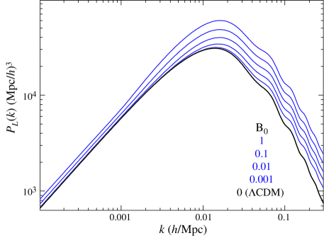
We show $P_{L}(k)$ for several choices of $B_{0}$ in Fig. 5. Despite the large change in amplitude at high $k$, the high $B_{0}$ models cannot be automatically ruled out by galaxy clustering data since the nearly multiplicative shift can be mimicked by galaxy bias. Likewise, non-linear measurements of the mass power spectrum through the cluster abundance, Lyman-$\alpha$ forest, and cosmic shear also cannot be straightforwardly applied. As the local curvature exceeds the background curvature in collapsed dark matter halos one would expect the gravitational dynamics to return to Newtonian. For this reason, our predictions are restricted to the linear regime at $k\lesssim 0.1h$ Mpc^-1. We intend to explore these issues further in a future work.

Finally the cross correlation between the ISW effect and the angular power spectra of galaxies is markedly different in these models and potentially excludes large $B_{0}$ solutions. The angular power spectra of galaxies is given in the linear regime by

$$C^{g_{j}g_{j}}_{l}=4\pi\int\frac{dk}{k}[I^{g_{j}}_{l}(k)]^{2}{4\over 25}{k^{4}\over\Omega_{m}^{2}H_{0}^{4}}{k^{3}P_{\zeta_{i}}\over 2\pi^{2}},$$ (55)

where

$$I^{g_{j}}_{l}(k)=\int{d}zD_{G}(a,k){n_{j}(z)b_{j}(z)}j_{l}(kD)\,,$$ (56)

$n_{j}(z)$ is the galaxy redshift distribution normalized to $\int dzn_{j}=1$, and $b_{j}(z)$ is the galaxy bias.

The cross correlation between the CMB ISW effect and galaxies becomes

$$C^{g_{j}{\rm I}}_{l}=4\pi\int\frac{dk}{k}I^{g_{j}}_{l}(k)I^{\rm I}_{l}(k){6\over 25}{k^{2}\over\Omega_{m}H_{0}^{2}}{k^{3}P_{\zeta_{i}}\over 2\pi^{2}}\,.$$ (57)

The correlation coefficient between the total temperature anisotropy and the galaxies is given by

$$R_{l}\equiv{C_{l}^{g_{j}{\rm I}}\over\sqrt{C_{l}^{TT}C_{l}^{g_{j}g_{j}}}}$$ (58)

and is independent of the galaxy bias if it is slowly varying with redshift. We have neglected galaxy magnification bias which leads to an additional source of correlation.

For definiteness, we assume that the galaxy sets come from a net galaxy distribution of

$$n_{g}(z)\propto z^{2}e^{-(z/1.5)^{2}}\,,$$ (59)

which is further partitioned by photometric redshift into several galaxy samples,

$$n_{j}(z)\propto n_{g}(z)\left[{\rm erfc}\left(\frac{z_{j-1}-z}{\sqrt{2}\sigma(z)}\right)-{\rm erfc}\left(\frac{z_{j}-z}{\sqrt{2}\sigma(z)}\right)\right]\,,$$ (60)

where erfc is the complementary error function and $\sigma(z)=0.03(1+z)$ reflects the effect of photometric redshift scatter.

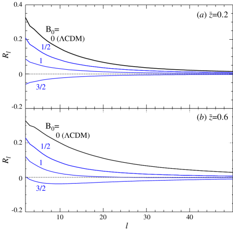
Fig. 6 shows the correlation coefficient for several values of $B_{0}$. We take two redshift bins from Eq. (60) partitioned by $z_{j}=0,0.4,0.8$ to achieve effective redshifts of $\bar{z}=0.2$ and $0.6$. Current observations constrain the correlation near $l\sim 20$ corresponding to scales which are an order of magnitude smaller than those contributing to the ISW quadrupole. Between $1/2\lesssim B_{0}\lesssim 1$ the galaxy-ISW correlation is substantially reduced. For $B_{0}\gtrsim 3/2$, galaxies are in fact anti-correlated with the CMB since $\Phi_{-}$ grows on the relevant scales. A loose bound from the observed correlation would therefore be $B_{0}\lesssim 3/2$ at the significance levels of the reported detections (e.g. Boughn and Crittenden (2004); Fosalba and Gaztanaga (2004); Scranton et al. (2004); Nolta et al. (2004); Afshordi et al. (2004); Giannantonio et al. (2006)) but we expect more detailed modeling to yield better constraints in the future. It is likely that a significant reduction of the large angle anisotropy from this mechanism could be excluded unless other sources, such as magnification bias, can generate the observed positive correlation.

Figure 6: Cross correlation coefficient between the CMB and galaxies in the $\Lambda$CDM expansion history. Shown are two representative redshift bins centered around $\bar{z}=0.2$ and $0.6$ with $B_{0}=0$  ($\Lambda$CDM), 1/2, 1, 3/2. The cross correlation is substantially reduced for $1/2\lesssim B_{0}\lesssim 1$ and becomes negative for $B_{0}\gtrsim 3/2$.

VII Discussion

We have studied the evolution of linear cosmological perturbations in $f(R)$ models for modified gravity in the physical—or Jordan—frame. Here the gravitational dynamics are fourth order and the matter is minimally coupled and separately conserved. For models that recover the Einstein-Hilbert action at high curvature $R$, we find that for each expansion history specified by $H(\ln a)$ there exists two branches of $f(R)$ solutions that are parameterized by $B\propto f_{RR}$, the second derivative of $f(R)$. For $B<0$, which includes most models previously considered Carroll et al. (2004); Zhang (2006), there is a short-timescale instability that prevents recovery of the general-relativistic expectations at high curvature that is important for maintaining agreement with CMB measurements.

For the stable $B>0$ branch, $f(R)$ models predict a rich set of linear phenomena that can be used to test such deviations from general relativity. For example, large $B\sim 1$ models lower the large-angle anisotropy of the CMB and may be useful for explaining the low quadrupole observed on our sky. They also predict qualitatively different correlations between the CMB and galaxy surveys which may provide the best upper limit on the deviations currently available. Smaller deviations in $B$ are observable at smaller scales through changes to the shape of the linear power spectrum. In the limit that $B\rightarrow 0$ and the expansion history is given by $\Lambda$CDM, linear perturbations in $f(R)$ models approach the general relativistic predictions exactly. We intend to examine constraints on $f(R)$ models in a future work.

More generally, this class of phenomenological $f(R)$ models provides insight on the types of deviations that might be expected from alternate metric theories of gravity in the linear regime. Conservation of the matter stress-energy tensor severely restricts the form of allowed deviations on both super- and sub- horizon scales Bertschinger (2006); Sawicki et al. (2006). Even if these $f(R)$ models prove not to be viable as a complete alternate theory of gravity that includes solar-system tests, they may serve as the basis for a “parameterized post-Friedmann” description of linear phenomena that parallels the parameterized post-Newtonian description of small-scale tests.

Acknowledgments: We thank Sean Carroll, Mark Hindmarsh, Michael Seifert, Kendrick Smith, Bob Wald, and the participants of the Benasque Cosmology Workshop and the Les Houches Summer School for useful conversations. This work was supported by the U.S. Dept. of Energy contract DE-FG02-90ER-40560. IS and WH are additionally supported by the David and Lucile Packard Foundation. This work was carried out at the KICP under NSF PHY-0114422.

References

- Carroll et al. (2004) S. M. Carroll, V. Duvvuri, M. Trodden, and M. S. Turner, Phys. Rev. D70, 043528 (2004), eprint astro-ph/0306438.
- Capozziello et al. (2003) S. Capozziello, S. Carloni, and A. Troisi (2003), eprint astro-ph/0303041.
- Nojiri and Odintsov (2003) S. Nojiri and S. D. Odintsov, Phys. Rev. D68, 123512 (2003), eprint hep-th/0307288.
- Dick (2004) R. Dick, Gen. Rel. Grav. 36, 217 (2004), eprint gr-qc/0307052.
- De Felice et al. (2006) A. De Felice, M. Hindmarsh, and M. Trodden, JCAP 0608, 005 (2006), eprint astro-ph/0604154.
- Chiba (2003) T. Chiba, Phys. Lett. B575, 1 (2003), eprint astro-ph/0307338.
- Multamaki and Vilja (2006a) T. Multamaki and I. Vilja, Phys. Rev. D74, 064022 (2006a), eprint astro-ph/0606373.
- Brevik et al. (2004) I. Brevik, S. Nojiri, S. D. Odintsov, and L. Vanzo, Phys. Rev. D70, 043520 (2004), eprint hep-th/0401073.
- Erickcek et al. (2006) A. L. Erickcek, T. L. Smith, and M. Kamionkowski (2006), eprint astro-ph/0610483.
- Cembranos (2006) J. A. R. Cembranos, Phys. Rev. D73, 064029 (2006), eprint gr-qc/0507039.
- Sotiriou (2006) T. P. Sotiriou, Gen. Rel. Grav. 38, 1407 (2006), eprint gr-qc/0507027.
- Shao et al. (2006) C.-G. Shao, R.-G. Cai, B. Wang, and R.-K. Su, Phys. Lett. B633, 164 (2006), eprint gr-qc/0511034.
- Faraoni (2006) V. Faraoni, Phys. Rev. D74, 023529 (2006), eprint gr-qc/0607016.
- Bardeen (1980) J. M. Bardeen, Phys. Rev. D 22, 1882 (1980).
- Hu and Eisenstein (1999) W. Hu and D. J. Eisenstein, Phys. Rev. D 59, 083509 (1999), eprint astro-ph/9809368.
- Bertschinger (2006) E. Bertschinger (2006), eprint astro-ph/0604485.
- Starobinsky (1980) A. A. Starobinsky, Phys. Lett. B91, 99 (1980).
- Multamaki and Vilja (2006b) T. Multamaki and I. Vilja, Phys. Rev. D73, 024018 (2006b), eprint astro-ph/0506692.
- Capozziello et al. (2006) S. Capozziello, S. Nojiri, S. D. Odintsov, and A. Troisi, Phys. Lett. B639, 135 (2006), eprint astro-ph/0604431.
- Nojiri and Odintsov (2006a) S. Nojiri and S. D. Odintsov (2006a), eprint hep-th/0608008.
- de la Cruz-Dombriz and Dobado (2006) A. de la Cruz-Dombriz and A. Dobado (2006), eprint gr-qc/0607118.
- Nojiri and Odintsov (2006b) S. Nojiri and S. D. Odintsov (2006b), eprint hep-th/0611071.
- Amendola et al. (2006a) L. Amendola, D. Polarski, and S. Tsujikawa (2006a), eprint astro-ph/0603703.
- Amendola et al. (2006b) L. Amendola, D. Polarski, and S. Tsujikawa (2006b), eprint astro-ph/0605384.
- Spergel et al. (2006) D. N. Spergel et al. (2006), eprint astro-ph/0603449.
- Dvali et al. (2000) G. R. Dvali, G. Gabadadze, and M. Porrati, Phys. Lett. B485, 208 (2000), eprint hep-th/0005016.
- Sawicki et al. (2006) I. Sawicki, Y. Song, and W. Hu, Phys. Rev. D submitted, astro (2006), eprint astro-ph/0606285.
- Hu (1998) W. Hu, Astrophys. J. 506, 485 (1998), eprint astro-ph/9801234.
- Dolgov and Kawasaki (2003) A. D. Dolgov and M. Kawasaki, Phys. Lett. B573, 1 (2003), eprint astro-ph/0307285.
- Woodard (2006) R. P. Woodard (2006), eprint astro-ph/0601672.
- Zhang (2006) P. Zhang, Phys. Rev. D73, 123504 (2006), eprint astro-ph/0511218.
- Siefert and Wald (2007) M. Siefert and R. Wald, in prep. (2007).
- Bean et al. (2006) R. Bean, D. Bernat, L. Pogosian, A. Silvestri, and M. Trodden (2006), eprint astro-ph/0611321.
- Faraoni (2005a) V. Faraoni, Phys. Rev. D72, 124005 (2005a), eprint gr-qc/0511094.
- Faraoni (2005b) V. Faraoni, Phys. Rev. D72, 061501 (2005b), eprint gr-qc/0509008.
- Boughn and Crittenden (2004) S. Boughn and R. Crittenden, Nature 427, 45 (2004).
- Fosalba and Gaztanaga (2004) P. Fosalba and E. Gaztanaga, Mon. Not. R. Astron. Soc. 350, 37 (2004).
- Scranton et al. (2004) R. Scranton et al., Astrophys. J. in press (2004), eprint astro-ph/0307335.
- Nolta et al. (2004) M. R. Nolta et al., Astrophys. J. 608, 10 (2004), eprint astro-ph/0305097.
- Afshordi et al. (2004) N. Afshordi, Y.-S. Loh, and M. Strauss, Phys. Rev. D 69, 083524 (2004).
- Giannantonio et al. (2006) T. Giannantonio et al., Phys. Rev. D74, 063520 (2006), eprint astro-ph/0607572.