TASS Mark IV Photometric Survey of the Northern Sky

Abstract

The Amateur Sky Survey (TASS) is a loose confederation of amateur and professional astronomers. We describe the design and construction of our Mark IV systems, a set of wide-field telescopes with CCD cameras which take simultaneous images in the $V$ and $I_{C}$ passbands. We explain our observational procedures and the pipeline which processes and reduces the images into lists of stellar positions and magnitudes. We have compiled a large database of measurements for stars in the northern celestial hemisphere with $V$-band magnitudes in the range $7<V<13$. This paper describes data taken over the four-year period starting November, 2001. One of our results is a catalog of repeated measurements on the Johnson-Cousins system for over 4.3 million stars.

1 Introduction

In recent years, the combination of relatively inexpensive CCD detectors and powerful desktop computers has made it possible for almost anyone to acquire and process very large amounts of astronomical information. Certain projects requiring large amounts of telescope time are impractical at heavily oversubscribed observatories, but can now be carried out by dedicated amateurs (Paczyński, 2000). Several years ago, we used modest equipment to perform a photometric survey of bright sources near the celestial equator (Richmond et al., 2000). The simple, fixed mounts and drift-scan technique of our Mark III systems limited that project to a small strip of the sky.

We have since constructed new mounts and switched to stare-mode observations, allowing us to cover nearly the entire northern celestial hemisphere. We report here on results from our Mark IV systems, which provide repeated $V$-band and $I_{C}$-band measurements of stars of intermediate brightness. Section 2 describes our equipment, section 3 our location and mode of operation, and section 4 the pipeline which extracts measurements from our images and performs preliminary calibration. After discovering systematic errors in our photometry, we attempted to remove their effects from some of the derived quantities in our database; section 5 explains these corrections. The resulting “patches catalog” provides a homogeneous network averaging 190 stars per square degree with $V$-band and $I_{C}$-band measurements of moderate precision: $\sim 0.05$ mag at the bright end, $\sim 0.20$ mag at the faint end.

Our survey may be most useful as a source of quick photometric calibration: it is dense enough to provide at least one star within the small field of view of typical CCD images, and its $I_{C}$-band measurements extend into the red end of the the visible portion of the spectrum, where some unfiltered systems are most sensitive. Our work is, of course, no replacement or substitute for primary photometric standards such as Landolt (1992), but may serve as a temporary measure if conditions do not permit the necessary all-sky observations. Studies of long-period, high-amplitude variable stars may also profit from our repeated measurements over several years.

2 Hardware

We describe here the detectors, optics, and mounts of our instruments; readers can skip to Table 1 for a summary. The Mark IV units are built around CCD chips designated Loral Fairchild CCD442A, which are $2048\times 2048$ arrays of 15-micron pixels. We designed and built our own electronics to read the sensors; they provide 16 bits of data per pixel with a readout time of 46 seconds. The gain of the CCDs is about 2.4 electrons per Analog-to-Data Unit (ADU), and the readnoise is about 15 electrons. We circulate water from a commercial chiller through thermoelectric coolers in each camera to keep the chips at a temperature fixed within 1 degree Celsius throughout each night; we vary this temperature depending on the ambient conditions, but it is typically $-20$ degrees C. The dark current at this temperature is about 0.2 electrons per second per pixel, which is negligible compared to contributions from the background sky. The CCDs are not isolated by a vacuum; instead, we pump dry air through the camera heads to prevent moisture from condensing into ice crystals on the silicon.

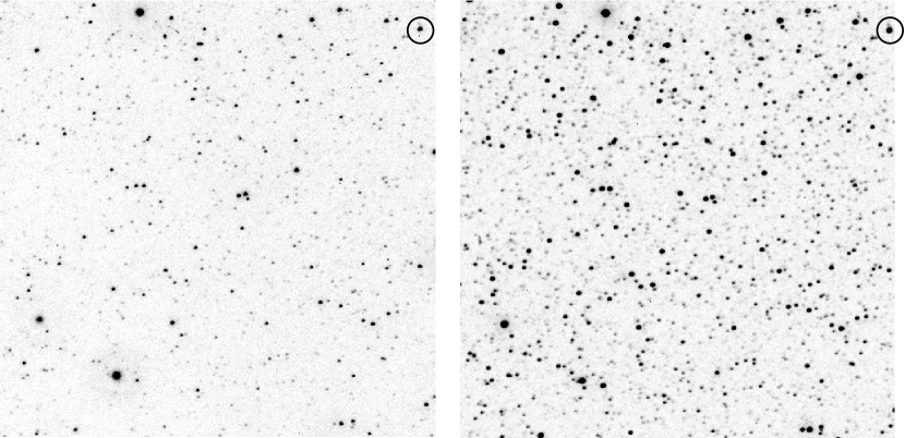
Figure 1: The central portion of a Mark IV image pair, a $1^{\circ}\times 1^{\circ}$ area centered at RA=20:16:14.2, Dec=+16:16:18, about 10 degrees from the galactic plane. $V$-band is on the left, $I_{C}$-band on the right. North is up, East to the left. The circled star is R Sge.

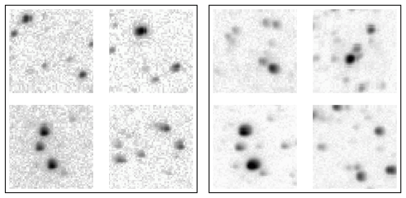
Figure 2: Closeups of the corners of a Mark IV image pair. The contrast is logarithmic to enhance features in the PSF. $V$-band is on the left, $I_{C}$-band on the right. North is up, East to the left.

Each CCD is mounted at the focus of its own small telescope. We designed 100mm f/4 custom refractive optics to provide small aberrations over a wide field for a particular range of wavelengths. Each lens has coatings optimized for its portion of the spectrum. The optics yield an image scale of 7.7 arcseconds per pixel and a field about 4.2 degrees on a side. The illumination of the focal plane is uniform to about $10\%$ across the width of the CCDs. Stellar images are slightly sharper at the center of the frame than near the edges, with a FWHM of $2.5-3.3$ pixels in $V$-band and $2.8-3.8$ pixels in $I_{C}$-band. This corresponds to $19-29$ arcseconds, far larger than the diffraction limit ($\sim 3^{{}^{\prime\prime}}$) or the local seeing ($\sim 3-6^{{}^{\prime\prime}}$). A portion of this excess blurring is due to the drive mechanism: many images show a slight elongation in the East-West direction, and the residuals of Mark IV positions from the Tycho-2 catalog (Høg et al., 2000) are slightly larger in the East-West direction than the North-South direction. The remainder of the PSF width is probably due to mediocre focusing: we do not adjust the focus as the temperature changes. The wide PSF does provide one benefit: it avoids the photometric complications of undersampled images (Bakos et al., 2004). Figure 1 shows the central portion of one pair of images, in a relatively dense star field, and figure 2 shows closeup subsections from each corner; note the slight elongation of the PSF away from the optical axis.

Each camera has its own filter mounted in front of the CCD. The filters were made by Omega Optical, Inc., according to the Bessell (1990) prescription. The shutter sits between the filter and the lens assembly; it has two sliding leaves which meet at the middle of the field and take 0.2 seconds to slide together or apart.

A single Mark IV unit consists of two telescopes — one $V$-band, one $I_{C}$-band — placed side-by-side on a common mount. The equatorial mount can cover Declinations ranging from the horizon to the pole, but has a limited range in Right Ascension: it can move only thirty degrees away from the meridian in either direction.

3 Operation

All the data described in this paper was collected from the roof of the first author’s home in Batavia, IL: latitude $41.8271$ North, longitude $88.3125$ West, altitude $217$ meters. This region of North America does not have very clear skies in general, as long experience at Yerkes Observatory (e.g., Cudworth, 1985) and other nearby sites has shown; moreover, the very bright lights of the Chicago metropolitan area are less than 50 km distant, and a large interstate highway lies 6 km to the south. We decided to acquire measurements as frequently as possible, and therefore observed at times through thin clouds and high humidity, and during all lunar phases. The bright glow and strong gradients in sky brightness are responsible for some of the systematic photometric errors described in section 5.

Three Mark IV units contributed measurements, each focusing on a different region of the sky. The unit “TOM1” acquired images centered on Declinations $-4<\delta<+16$ over the period 2001 Nov 11 to 2005 Nov 11; “TOM2” scanned the region $+20<\delta<+48$ over the period 2003 Apr 1 to 2005 Nov 17; and “TOM3” covered the area $+52<\delta<+88$ between 2003 Apr 9 and 2005 Nov 17. Each scan overlaps its neighbors to the South and North by about one quarter of a degree, so that the three units working together cover the entire Declination range seamlessly.

At the start of each night, the operator opens the telescope covers, points each unit to the meridian, and sets the Declination of each unit to the bottom of its range (i.e., TOM1 points to $\delta=-4$). The units then follow a strict pattern during the night: they take a set of images at fixed Right Ascension while moving upwards in Declination by steps of $4$ degrees. Exposure times were $100$ seconds from 2001 to 2004, and $200$ seconds during 2005. The systems require about $60$ seconds to read each set of images and slew to the next position. After reaching the northern limit of its region, each unit returns to the southern limit and returns to the meridian. The result is a set of slightly overlapping images which sample the sky as it crosses the meridian. Each unit acquires about 20 ($V$, $I_{C}$) image pairs per hour, which correspond to about 660 MBytes of raw data.

Over the course of many nights, therefore, the survey images occur at the same Declinations (centered at $\delta=-4,0,+4,+8,...$). However, the starting position in Right Ascension was not set according to any rule prior to 2005, and thus the Right Ascension centers of those survey images vary randomly from one night to the next. As a consequence, stars in those images appear at roughly the same image coordinate in one direction (from North to South), but cover the entire range of image coordinates in the other direction (from East to West). We did fix the Right Ascension centers starting in 2005.

In the morning, the operator closes the telescope covers and stows the units. He then visually inspects five to ten percent of the images taken during the night, as well as the results of the pipeline processing which has finished so far. The software will find and flag some problems, such as periods of clouds during the night, but other problems, such as ice crystals forming on the CCD, are better found by a human. If there is evidence for very poor sky conditions or equipment problems, the entire night’s data is discarded. Individual images with obvious problems are also deleted at this point. Otherwise, the operator waits for the analysis software to complete its task, then backs up the results.

After several months of experience, we learned that we can control the temperature of the CCDs well enough that dark frames need not be taken every night; we find that a new set every month is sufficient. We also noticed that our flatfield frames, made from a median of many target images on a good night, varied very little from night to night; therefore, we update our flatfield frames only when necessary: that means whenever we make adjustments to the equipment, or when the visible appearance of the raw images changes noticeably (e.g., due to shifting dust specks), or about once per month by default.

4 Software

We have written our own software to reduce the raw images into lists of stars with measured properties. Some of it has grown from the PCVista package (Treffers & Richmond, 1989), some of it was created specifically for this survey. All the software is available freely online; contact the second author for details. We believe that one particular module may be of use to other astronomers, so we describe it at some length in the Appendix.

The reduction procedure involves four basic steps: creating master darks and flats, applying them to target images, finding stars and measuring their instrumental properties, and converting the instrumental units to standard ones. We describe each step briefly below.

To create master dark frames, we take a series of at least ten images of the same length as our target images, with the dome open and the cameras near the middle of their declination range, but with the camera shutters closed. The temperature of the CCD is controlled to be the same during these dark frames as it is during normal observations. We compute the interquartile mean at each pixel location and place it into the master dark frame. To create master flatfield frames, we start with a series of 38 target images taken during a good night. The bright skies in Batavia provide 3000 to 10000 photoelectrons per pixel in the background of each image, so the statistical variations in the combined signal of each pixel are less than $0.3\%$. We use a strip of prescan columns to check for any fixed offset between these target frames and the master dark image; if a difference exists, we subtract it from all pixels in the target images. We then subtract the master dark frame from each target image, and then compute the pixel-by-pixel interquartile mean from the set of all target images to serve as the master flatfield frame. We scan each master flatfield frame for small regions of connected pixels which lie far from the local mean value, due to chip defects, dust or ice crystals, and create a mask of all such bad regions. We later flag any detected objects which touch these bad regions.

In order to clean a raw target image, we first compare its prescan columns to the master dark frame’s prescan columns; if a difference exists, we shift the target image’s pixels by the mean difference. We then subtract the master dark frame from the target image. We divide the resulting target frame by a normalized version of the master flatfield image. We fit a gaussian to the histogram of pixel values in the cleaned image to estimate the sky level; images with sky values outside a particular range are discarded. We remove large-scale variations in the sky background (due to clouds or lights in neighboring houses) by fitting a first-order polynomial to local sky measurements on a $10\times 10$ grid and subtracting the model from the image.

We search for stars in a cleaned image by marking as candidates all pixels exceeding a fixed threshold above the sky and measuring their properties; candidates which pass a series of tests based on Full-Width at Half Maximum (FWHM), sharpness and roundness (Stetson, 1987) are designated as stars. We then measure each star’s position on the image by fitting one-dimensional gaussians to the intensity-weighted marginal sums of pixels in each direction. We calculate the instrumental magnitude of each star using a fixed circular aperture of radius $4$ pixels ($30^{{}^{\prime\prime}}$) and local sky measured as the median of values in an annulus of radii $10$ and $20$ pixels ($77^{{}^{\prime\prime}}$ and $154^{{}^{\prime\prime}}$). The uncertainty in this magnitude is estimated using the statistics of electrons within the aperture (Howell, 1989). We set flags for any measurement which is likely to be unreliable, if it is close to the edge of an image, touches a bad region, contains saturated pixels, etc.

In order to transform the $(x,y)$ pixel positions of objects into $(\rm{RA},\rm{Dec})$, we create a reference catalog by selecting roughly 80% of the stars from the Tycho-2 catalog (Høg et al., 2000), those which meet the “astrometry” criteria listed in table 2. There are typically 50 such stars per image. For each image, we use the match software (see Appendix) to match the reference stars to detected objects, fit a cubic model to the transformation between image $(x,y)$ and projected $(\rm{RA},\rm{Dec})$ coordinates, and apply that model to the positions of all detected objects. The residuals from the model range from $\sim 0{\hbox to0.0pt{.\hss}}^{{}^{\prime\prime}}8$ for bright ($V<10$) stars to $\sim 3{\hbox to0.0pt{.\hss}}^{{}^{\prime\prime}}5$ for faint ($V>13$) stars. Our matching routines fail in regions very close to the celestial pole, forcing us to discard measurements with Declinations above $+88\hbox to0.0pt{.\hss}^{\circ}2$.

We apply a preliminary photometric calibration to measurements in the final stage of the pipeline. We again choose Tycho-2 as our reference, but create a second subset with more stringent limits (see table 2); this yields roughly 10 to 15 reference stars in each Mark IV image. We convert the Tycho-2 measurements in $B_{T}$ and $V_{T}$ to the Johnson-Cousins $V$ and $I_{C}$ magnitudes using relationships kindly provided by Arne Henden (Henden, 2001) and shown in table 3. We discard any stars not detected simultaneously in both $V$ and $I$. We then create photometric solutions for each night with the following form:

$$V = v+a_{j}+b*(v-i)-k_{V}*X$$ (1)

$$I_{C} = i+c_{j}+d*(v-i)-k_{I}*X$$ (2)

where $V$ and $I_{C}$ are the calibrated magnitudes of a star, $v$ and $i$ the instrumental measurements, $a_{j}$ and $c_{j}$ the zero points of the $j$-th images during the night, $b$ and $d$ color terms, $k_{V}$ and $k_{I}$ the first-order extinction coefficients, and $X$ the airmass of each star. Note that we allow the zero-points to vary from one image to the next, but assume single color terms for the entire night. Differential extinction can be significant over a single frame, which may span a range of up to 0.12 airmasses, but our limited range of observations does not allow us to solve for it reliably; we therefore assume fixed values of $k_{V}=0.20$ and $k_{I}=0.06$. If the actual extinction coefficients were twice as large as our adopted values, the maximum error across a single frame would be about $0.020$ mag in $V$-band and about $0.007$ mag in $I_{C}$-band for objects near the southern and northern limits of our survey.

The output of the pipeline is a list of stars detected simultaneously by both cameras of a single Mark IV unit, with (RA, Dec) positions and preliminary ($V$, $I_{C}$) magnitudes. A good night yields several thousand stars per image and (near the equinoxes) about 400 images. At intervals of roughly one month, we place these measurements into the Mark IV engineering database, where they are freely available. The software is robust enough that it can run to completion even during mediocre observing conditions, causing a small amount of poor quality data to enter the database. We warn the potential user not to accept blindly the results of every query; checking individual measurements against those of nearby stars and those from other nights can help to identify bad data. We also note that the preliminary magnitudes stored in this database suffer from small systematic errors, which we describe in the following section.

5 The “patches” catalog

For some purposes, the measurements produced by the pipeline and stuffed into the engineering database are good enough; in figure 3, one can see clearly the light curve of the long-term, large-amplitude variable star R Sge. For others, however, it is necessary to improve the photometric calibration of the Mark IV results. We describe here a subset of the Mark IV data which we subject to additional analysis; the end result will be a catalog of mean properties of stars which were measured many times. We believe that this “patches catalog” will be more useful to most members of the community than the individual measurements in the engineering database.

5.1 Selecting stars for further analysis

We began with all measurements made over the period 2001 Nov 11 to 2005 Nov 17. Our first step was to remove spurious and unreliable detections by selecting objects which were detected many times. We chose stars detected in at least 5 pairs of $V,I$ images (though we had to decrease this threshold to 3 detections in three isolated degree-sized regions of the sky with poor coverage). The result is a set of roughly 4.3 million stars, with magnitudes roughly in the range $7<V<13$ (figure 4). The mean number of measurement pairs for each star is 37, but the distribution has a long tail; see figure 5.

During our analysis of this dataset, we found frequent outliers in the Mark IV measurements, due to clouds, cosmic rays, satellite trails, passing airplanes, and other image defects. In order to reduce their influence on the majority of the measurements, we will frequently employ an interquartile mean (IQM) to determine average values. We form the IQM by sorting all magnitude measurements, discarding the top 25% and bottom 25% of the distribution, and computing the mean of the remaining values.

5.2 Additional photometric calibration

In order to check the accuracy of our photometry, we matched the stars in the “patch” dataset against stars measured by Landolt (Landolt, 1983, 1992). Because the Mark IV cameras have pixels over $7^{{}^{\prime\prime}}$ in size and we measure light in apertures of radius $30^{{}^{\prime\prime}}$, our measurements blend together light from stars within roughly one arcminute of each other; for comparison, Landolt made his measurements through considerably smaller apertures, $13^{{}^{\prime\prime}}$ and $7^{{}^{\prime\prime}}$ in radius. We used the Vizier facility to check each Landolt star for significant neighbors, which we define as stars from the USNO B1.0 catalog (Monet et al., 2003) within $70^{{}^{\prime\prime}}$ and $2$ magnitudes of the Landolt star. Stars with significant neighbors were discarded. We also checked each Landolt star for variability using the GCVS version 4.2 (Samus et al., 2004); we discarded any star even suspected of being variable. We examined the Mark IV record for each remaining Landolt star and discarded any objects with significant variability. There are 153 isolated, constant Landolt stars which match items in the “patches” dataset; these are shown as small symbols in the figures below. Some of these are so bright that they saturate the Mark IV detectors, or so faint that their measurements have very large scatter. For some purposes, we will consider only the 99 stars in the range $8.0<V<12.5$ and $7.5<I_{C}<12.5$, which have accurate and reasonably precise Mark IV photometry; we denote them with large symbols.

The differences between the Landolt magnitudes of these stars and the IQM of Mark IV magnitudes are shown as a function of magnitude in figures  6 and 7, and as a function of ($V-I_{C}$) color in figures  8 and 9. There is clearly a color-dependent error in the $V$-band measurements, and a fixed offset in the $I_{C}$-band measurements. We made unweighted linear fits to the residuals in the reliable subset to derive the following corrections,

$$V_{\rm cor} = V_{\rm eng}-0.0353+0.09362*(V_{\rm eng}-I_{\rm eng})$$ (3)

$$I_{\rm cor} = I_{\rm eng}-0.0503$$ (4)

where $V_{\rm eng}$ and $I_{\rm eng}$ are the interquartile means of values in the Mark IV engineering database, and $V_{\rm cor}$ and $I_{\rm cor}$ are the corrected values. Table 4 lists the statistics of the differences between Landolt photometry and the corrected Mark IV photometry; we show the residuals as a function of magnitude in figure 10 and figure 11, and as a function of ($V-I_{C}$) color in figure 12 and figure 13.

After these corrections, we note that the errors in Mark IV photometry do not show the usual pattern of increasing gradually from bright stars to faint stars; instead, the errors seem independent of magnitude. Calculation of the errors based on photon statistics and sensor properties yield values which are much smaller than the observed errors for bright stars; for example, we expect the uncertainty per measurement to be less than $0.01$ mag for stars of $V\leq 10$. Why do the measurements fail to meet these predictions?

One reason is the relatively low precision of the preliminary photometric calibration. As table 2 indicates, we accepted Tycho-2 stars with estimated uncertainties of up to $0.05$ mag to serve as references in our pipeline processing; it was the only way to ensure a reasonable number of reference stars in every image. In addition, the particular set of Tycho-2 stars used to calibrate one particular target star varied during the first three years of the survey since the Right Ascension of image centers drifted randomly from night to night. It is possible that this changing mix of references could add some noise to the overall photometric calibration. However, we note that in 2005, when the Right Ascension centers of images were fixed, and a uniform set of reference stars did appear repeatedly for each target star, the internal scatter of our measurements did not decrease significantly. We do know of one additional and significant source of error: systematic variations in photometry as a function of position in the focal plane, as we will demonstrate in the next section.

5.3 Using patches to reduce systematic errors

It is not an easy matter to measure precisely the brightness of astronomical sources over a wide field: optics deliver a variable illumination and a variable PSF to the focal plane, and the sky brightness varies significantly across the field. Systematic errors may easily dominate the error budget for bright sources, as in, for example, the Digitized Second Palomar Observatory Sky Survey (Gal et al., 2004), the ROTSE-I survey (Akerlof et al., 2000), or the All Sky Automated Survey (Pojmański, 2002) (see figure 14). If one chooses a fixed set of field centers and points to them accurately, then each star may suffer the same error repeatedly, and thus the scatter of individual measurements around the mean will be small. This satisfies the needs of some projects, such as searching for variable stars; but for other goals, such as creating a uniform set of photometric reference stars, one must remove the errors in mean values which remain over the field of view.

The Mark IV survey was carried out so that cameras returned to nearly the same Declination each night, but (for a large fraction of the survey) varied in Right Ascension in an irregular fashion. Thus, photometric errors due to location in the focal plane would appear in a complicated manner. Consider two identical stars separated by $\sim 2^{\circ}$ on the sky (about half the size of one image) in the North-South direction; one might be incorrectly measured as $0.04$ mag brighter than the other, night after night after night. On the other hand, measurements of two identical stars separated by $\sim 2^{\circ}$ in the East-West direction would depend on the exact pointing of each night’s image: on one night, the eastern star might fall near the image center and the western star near the edge, causing the eastern star to appear $0.04$ mag brighter; but the next night, the eastern star might be near the edge and the western star near the center, causing the eastern star to appear $0.04$ mag fainter.

Ordinary flatfielding procedures such as ours can and do remove variations in sensitivity on very small spatial scales – among neighboring pixels – but fail to correct variations on larger spatial scale; indeed, if scattered light enters the optics, using a flatfield based on diffuse background light can introduce photometric errors in the measurements of point sources (Manfroid, 1995). The scatter between repeated measurements of bright stars in our engineering database, roughly $\sim 0.05$ mag, is half the center-to-edge variation in illumination from our optics (about $10\%$), suggesting that our flatfielding procedure may have introduced much of the error. Since we assign a single magnitude zero-point to all the stars in each image during our reductions, there is no way for our standard processing to account for such large-scale, position-dependent variations in sensitivity.

As Manfroid (1995) shows, it is possible to characterize these large-scale photometric errors by taking a special set of images arranged in a grid centered on a rich star field. In late 2002, we used the TOM1 unit to acquire images in a $7\times 7$ grid at four locations near the galactic plane. Our analysis of the grid images (see figure 15) reveals a pattern of residuals which has a significant change in Declination but varies little in Right Ascension, as one would expect from the fixed-Dec, variable-RA positions of fields during much of our survey. The gradient in Declination is due in large part to the bright sky at our site; since we always observe near the meridian, the bright horizon is always located in the same direction: to the South, for images taken at Declinations $\delta<+42^{\circ}$, or to the North, for images taken at Declinations $\delta>+42^{\circ}$. In the future, we hope to make similar maps of the residuals in the other two Mark IV units, check the maps to verify that they have been stable over the course of survey, and then apply them to all the measurements in the engineering database.

Although we cannot at the current time correct our photometry for these systematic errors, we can reduce the effect of those errors on certain statistical properties of our measurements. As figure 15 shows, the residuals change gradually across the $4{\hbox to0.0pt{.\hss}}^{\circ}2$ field of view. Suppose that we concentrate on the stars within a small portion of the field, one degree on a side. To first order, all the stars in this little region will suffer the same error in measurement each night. If we perform differential photometry of the stars in this region alone, we can recover any variations in the light of one star relative to its neighbors. The mean magnitudes of stars in the region will remain uncertain, but we may improve our knowledge of each star’s intrinsic variation around that mean.

The notion of dividing measurements made across a wide field of view into small groups is not a new one: Taff (1989) and Bucciarelli et al. (1992) describe the benefits of “imaginary subplates” for astrometry derived from Schmidt plates.

We divided all the measurements in our engineering database into “patches” one degree on a side; each patch overlaps its neighbors by one-quarter of a degree. The measurements in each patch define an inhomogeneous ensemble, since faint stars may not be detected as frequently as bright ones. Following the methods of Honeycutt (1992), we allowed the magnitudes from each image to shift up or down slightly in order to minimize the overall differences between measurements of the same stars. The main result for our purposes is the standard deviation from the mean ensemble magnitude for each star. As we show in figure 16 and figure 17, the standard deviation from the mean magnitude decreases significantly after ensemble processing: the floor of the distribution for bright stars shrinks from $\sim 0.05$ mag to $\sim 0.02$ mag in both passbands.

Another indication of the improvement offered by ensemble photometry is visible in figure 18, which shows the light curve of R Sge folded according to its period in the GCVS (Samus et al., 2004). The entire set of measurements in the engineering database (open symbols) includes several outliers, and the width of the locus is considerable. The ensemble procedure (filled symbols) discards data from several nights deemed to have residuals of larger size than usual, and brings the remaining measurements into better agreement.

5.4 Construction of the “patches” catalog

The “patches” catalog provides a short summary of the Mark IV survey: it contains mean positions and magnitudes for a subset of the most reliable detections: stars seen in a simultaneous ($V$, $I_{C}$) image pair on at least five occasions. We also compute several statistics which indicate for each star its degree of variability in our measurements. Readers may query the engineering database for the full (uncorrected, pre-ensemble) photometry of any stars of interest.

We can estimate the variability of a star in two ways. First, the ensemble photometry procedure produces not only a mean differential magnitude for each star, but also the standard deviation of the adjusted measurements around that mean (henceforth called $\sigma$). This is the quantity plotted on the ordinate of figure 16 and figure 17. We divide the stars into bins by magnitude and compute the median of $\sigma$ within each bin, as well as the range $r$ between the first and third quartiles. We then fit a parabolic model to the median values as a function of magnitude. In order to find stars which vary much more than the typical amount, stars which would lie far above the main locus in the graph of $\sigma$ versus magnitude, we compute a quantity we denote $\mathcal{D}$ (for its similarity to the normal deviate) as follows:

$${\mathcal{D}}={{{\sigma}-{\sigma_{p}}}\over{r}}$$ (5)

where $\sigma$ is the standard deviation of some star around its ensemble mean, $\sigma_{p}$ is the predicted standard deviation from our model, and $r$ is the average width of the locus in the $\sigma$ versus magnitude graph. In essence, $\mathcal{D}$ is a normalized measure of the degree to which a star varies more than the typical star in the ensemble. Since the ensemble solutions for each passband are independent, each star is assigned two values of $\mathcal{D}$. In figure 19, we show the distribution of $\mathcal{D}$ in each passband; the long tails of positive values contain candidates for variability.

Another measure of variability combines the information from the two passbands: the Welch-Stetson variability index (Welch & Stetson, 1993) assumes that changes in a star’s luminosity occur nearly simultaneously at all optical wavelengths. We use the ensemble output to compute a slightly modified version of the Welch-Stetson statistic which we shall call $\mathcal{W}$:

$$\mathcal{W}\equiv{\sqrt{{n}\over{n-1}}}\thinspace\thinspace{\sum_{i=1}^{n}{{\left(\left({{V_{i}-\bar{V}}\over{\sigma_{V}}}\right)\left({{I_{i}-\bar{I}}\over{\sigma_{I}}}\right)\right)}}}$$ (6)

Here $V_{i}$ is the $V$-band ensemble measurement of a star in the $i$-th image, and $\bar{V}$ the ensemble mean magnitude of the star; the weighting factor $\sigma_{V}$ is determined from the typical scatter from the ensemble mean for stars of similar brightness. The $I_{i}$, $\bar{I}$ and $\sigma_{I}$ symbols refer to the analogous quantities in the $I_{C}$-band ensemble. The distribution of $\mathcal{W}$ (figure 20) shows the same sort of long positive tail as figure 19; some of these outliers are due to intrinsic stellar variability, others due to erroneous measurements.

Because the Mark IV images have relatively large pixels ($7^{{}^{\prime\prime}}$ on a side), and because we use a large synthetic aperture ($30^{{}^{\prime\prime}}$ in radius) to measure them, a significant fraction of our measurements are contaminated by neighboring stars. In order to flag stars with possible contamination, we have looked for nearby companions to each star, using the survey itself as a reference. We checked for neighbors within two distances: $30^{{}^{\prime\prime}}$ and $60^{{}^{\prime\prime}}$. We assign a “proximity code” to each star following the rules listed in table 5. For example, a star which has two fainter neighbors at distances of $18^{{}^{\prime\prime}}$ and $27^{{}^{\prime\prime}}$, and one brighter neighbor at a distance of $45^{{}^{\prime\prime}}$, would be assigned a proximity code of 6. Neighbors which are too close for our equipment to resolve, or too faint for our equipment to detect, will not be flagged by this procedure. We find that roughly $0.3\%$ of the stars in our catalog are marked as having neighbors within $30^{{}^{\prime\prime}}$ and roughly $6.6\%$ marked as having neighbors within $60^{{}^{\prime\prime}}$. Our measurements for any of these stars may be unreliable.

The final version of our catalog appears in table 6. It contains 4,353,670 stars with Declinations in the range $-5.5<\delta<+88.2$.

6 Conclusion

Using wide-field telescopes and cameras of our own design, we have measured stars in the rough range $7\sim V<13$ over a four-year period in the Johnson-Cousins $V$ and $I_{C}$ passbands. All of our measurements are freely available in a database which may be queried over the Internet. We have selected a subset of objects observed multiple times, performed extra photometric calibration, and computed statistical indications of variability to create the “Mark IV patches catalog.”

We believe that this catalog will be especially useful to

• calibrate comparison stars in the fields of variable stars, supernovae, and gamma-ray bursts

• provide a net of photometric comparison stars for moving objects

• study variable stars of large amplitude

• verify that certain stars do not vary above a certain level

We remind the reader that our survey does suffer certain shortcomings: its large pixels make object detection and measurement unreliable in even moderately crowded fields, its photometric measurements contain systematic errors at the level of about five percent, and the engineering database contains some data taken in poor conditions. We chose to acquire very large amounts of information from a suburban site rather than to scan small pieces of the sky from a clear, dark site, based in part upon our available resources.

The Mark IV survey continues to collect data: at the time of writing (September 2006), the engineering database contained over 190 million measurements. We will continue to make our data available in several formats to the community at large for the foreseeable future.

Appendix A The match package

We describe here in some detail the procedure we use to calibrate the positions of objects in our images, since the task is a common one and other astronomers may be able to adapt our software to meet their needs (as the SHASSA (Gaustad et al., 2001) and ACS (Blakeslee et al., 2003) teams already have). Detailed documentation and the full source code can be found on-line or by contacting the second author.

The task is to convert the pixel coordinates $(x,y)$ of a list of objects found in some image to celestial coordinates $(\alpha,\delta)$. We assume that the user has a reference catalog of objects with celestial coordinates which overlaps substantially (and preferably surrounds) the detected objects. We break the job into five steps:

1. Project the reference objects onto a plane, converting $(\alpha,\delta)$ into standard coordinates $(\xi,\eta)$

2. Match the detected objects to the reference objects

3. Find the transformation which takes pixel coordinates $(x,y)$ to standard coordinates $(\xi,\eta)$

4. Apply the transformation to all the detected objects

5. De-project the $(\xi,\eta)$ coordinates of the detected object onto the celestial sphere, yielding their $(\alpha,\delta)$ positions

Our package contains short functions to perform the first and last steps, which involve nothing more than a bit of spherical trigonometry. The real work lies in the second step: finding the best set of matches between the detected and reference objects. We follow the method described by Valdes et al. (1995). It creates one set of triangles using the detected objects, a second set of triangles using the reference objects, then searches for similar triangles. The strength of this technique is its insensitivity to rotation, translation, inversion and differences in scale between the two lists of objects; its main weakness is that the computing time required to find a match grows as the total number of objects raised to sixth power.

Our implementation provides three standalone programs: project_coords performs the first step, match steps two through three, and apply_match steps four and five. In order to make the software flexible and easily incorporated into existing frameworks without modifying its source code, we have given the match program many command-line options, permitting the user to place contraints on the number of objects matched, the range of relative scale factors of the two lists, the critical matching radius, the number of iterations to make, etc. One can also request various amounts of diagnostic output from the routine to verify that a valid match was found. The software runs quickly enough to meet our needs for the Mark IV survey: it can match two lists of 100 objects in a few seconds on a typical desktop computer.

Figure 3: Light curve of R Sge, using all measurements in the Mark IV engineering database.

Figure 4: Distribution of magnitudes for stars in the “patches” dataset.

Figure 5: Distribution of number of observations for stars in the “patches” dataset.

Figure 6: Differences in $V$-band between Landolt photometry and interquartile mean values from the Mark IV engineering database .

Figure 7: Differences in $I_{C}$-band between Landolt photometry and interquartile mean values from the Mark IV engineering database .

Figure 8: Differences in $V$-band between Landolt photometry and Mark IV engineering photometry as a function of stellar color .

Figure 9: Differences in $I_{C}$-band between Landolt photometry and Mark IV engineering photometry as a function of stellar color .

Figure 10: Differences in $V$-band between Landolt photometry and corrected Mark IV magnitudes .

Figure 11: Differences in $I_{C}$-band between Landolt photometry and corrected Mark IV magnitudes .

Figure 12: Differences in $V$-band between Landolt photometry and corrected Mark IV magnitudes as a function of stellar color .

Figure 13: Differences in $I_{C}$-band between Landolt photometry and corrected Mark IV magnitudes as a function of stellar color .

Figure 14: Differences from Landolt photometry in $V$-band for Mark IV corrected measurements and ASAS3 measurements .

Figure 15: Residuals in $V$-band photometry in a special series of “grid calibration” images taken by the TOM1 unit in November, 2002. The $I_{C}$-band residuals show a similar pattern.

Figure 16: Scatter from the mean $V$-band magnitude in repeated measurements, before and after ensemble photometry. For clarity, only a small random subset of the entire dataset has been plotted.

Figure 17: Scatter from the mean $I_{C}$-band magnitude in repeated measurements, before and after ensemble photometry. For clarity, only a small random subset of the entire dataset has been plotted.

Figure 18: Phased light curve of R Sge, showing the difference between measurements in the engineering database (open symbols) and after ensemble photometry (filled symbols)..

Figure 19: Histogram of the normalized deviation from the ensemble median magnitude.

Figure 20: Histogram of the Welch-Stetson variability index $\mathcal{W}$.

Table 1: Summary of Mark IV hardware

CCD chip	Loral Fairchild CCD442A
pixels per chip	$2048\times 2048$, each $15\mu\times 15\mu$
gain	$2.4e^{-}$ per ADU
readout noise	$15e^{-}$
operating temperature	$-20\thinspace^{\circ}{\rm C}$
dark current	$0.2e^{-}$ per second per pixel
optics	$100{\rm mm\ }f/4$
plate scale	$7{\hbox to0.0pt{.\hss}}^{{}^{\prime\prime}}7$ per pixel
field of view	$4{\hbox to0.0pt{.\hss}}^{\circ}2\times 4{\hbox to0.0pt{.\hss}}^{\circ}2$

Table 2: Subsets of the Tycho-2 catalog (Høg et al., 2000)

property	astrometric subset	photometric subset
$B_{T}$ magnitude	$1.0<B_{T}$	$1.0<B_{T}<11.8$
$V_{T}$ magnitude	$1.0<V_{T}$	$1.0<V_{T}<10.7$
uncertainty in $B_{T}$	$\sigma(B_{T})<0.20$	$\sigma(B_{T})<0.05$
uncertainty in $V_{T}$	$\sigma(V_{T})<0.20$	$\sigma(V_{T})<0.05$
color	$-0.2<(B_{T}-V_{T})<1.8$	$-0.2<(B_{T}-V_{T})<1.8$
no other Tycho star	within $20^{{}^{\prime\prime}}$	within $50^{{}^{\prime\prime}}$
flags	not a double	not a double
number of stars	1475875	360741

Table 3: Converting Tycho-2 magnitudes to the Johnson-Cousins scale

Johnson-Cousins	Tycho-2
$B$	$B_{T}+0.018-0.2580(B_{T}-V_{T})$
$V$	$V_{T}+0.008-0.0988(B_{T}-V_{T})$
$R_{C}$	$V_{T}-0.014-0.5405(B_{T}-V_{T})$
$I_{C}$	$V_{T}-0.039-0.9376(B_{T}-V_{T})$

Table 4: Differences between Landolt and corrected Mark IV photometry

	N	$(V_{\rm Landolt}-V_{\rm cor})$	N	$(I_{\rm Landolt}-I_{\rm cor})$
unclipped	99	$-0.016\pm 0.036$	99	$-0.011\pm 0.035$
clipped	94	$-0.014\pm 0.031$	92	$-0.006\pm 0.024$

Table 5: How to compute the proximity code for a target star

If $\geq 1$ neighbor within	which is	then add
$30^{{}^{\prime\prime}}$	brighter than target	8
$30^{{}^{\prime\prime}}$	fainter than target	4
$60^{{}^{\prime\prime}}$	brighter than target	2
$60^{{}^{\prime\prime}}$	fainter than target	1

Table 6: Mark IV patches catalog

TASS ID	N	RA	$\sigma({\rm RA})$	Dec	$\sigma({\rm Dec})$	V	$\sigma(V)$	V ens $\sigma$	I	$\sigma(I)$	I ens $\sigma$	$\mathcal{D}_{V}$	$\mathcal{D}_{I}$	$\mathcal{W}$	prox
397943	58	0.00042	0.00018	-5.49426	0.00016	9.285	0.088	0.041	8.194	0.030	0.022	0.21	0.45	-0.07	0
398770	23	0.00061	0.00063	5.38051	0.00062	13.246	0.158	0.138	12.025	0.099	0.072	-0.26	-0.02	0.40	0
366763	64	0.00085	0.00012	1.08900	0.00008	9.095	0.044	0.027	8.561	0.023	0.022	-0.59	-0.42	0.57	0
398771	30	0.00116	0.00050	3.02078	0.00070	13.030	0.133	0.112	12.162	0.065	0.055	-0.46	-1.31	0.22	0

Note. — Table 6 is published in its entirety in the electronic edition of the PASP. A portion is shown here for guidance regarding its form and content.

References

- Akerlof et al. (2000) Akerlof, C., et al. 2000, AJ, 119, 1901
- Bakos et al. (2004) Bakos, G., et al. 2004, PASP, 116, 266
- Blakeslee et al. (2003) Blakeslee, J. P., et al. 2003, ASP Conf. Ser. 295, Astronomical Data Analysis Software and Systems XII, ed. H. E. Payne, R. I. Jedrzejewski & R. N. Hook, (San Francisco: ASP), 257
- Bessell (1990) Bessell, M. S. 1990, PASP, 102, 1181
- Bucciarelli et al. (1992) Bucciarelli, B., et al. 1992, AJ, 103, 1689
- Cudworth (1985) Cudworth, K. M. 1985, AJ, 90, 65
- Gal et al. (2004) Gal, R. R., et al. 2004, AJ, 128, 3082
- Gaustad et al. (2001) Gaustad, J. E., et al. 2001, PASP, 113, 1326
- Henden (2001) Henden, A. 2001, private communication
- Høg et al. (2000) Høg, E., et al. 2000, A&A, 355, L27
- Honeycutt (1992) Honeycutt, R. K. 1992, PASP, 104, 435
- Howell (1989) Howell, S. B. 1989, PASP, 101, 616
- Landolt (1983) Landolt, A. U. 1983, AJ, 88, 439
- Landolt (1992) Landolt, A. U. 1992, AJ, 104, 340
- Maddox, Efstathiou & Sutherland (1990) Maddox, S. J., Efstathiou, G., & Sutherland, W. J. 1990, MNRAS, 246, 433
- Manfroid (1995) Manfroid, J. 1995, A&AS, 113, 587
- Monet et al. (2003) Monet, D. G., et al. 2003, AJ, 125, 984
- Paczyński (2000) Paczyński, B. 2000, PASP, 112, 1281
- Pojmański (2002) Pojmański, G. 2002, Acta Astronomica, 52, 397
- Richmond et al. (2000) Richmond, M. W. et al. 2000, PASP, 112, 397
- Samus et al. (2004) Samus, N. N., et al. 2004, http://www.sai.msu.su/groups/cluster/gcvs/gcvs/
- Stetson (1987) Stetson, P. B. 1987, PASP, 99, 191
- Taff (1989) Taff, L. G. 1989, AJ, 98, 1912
- Treffers & Richmond (1989) Treffers, R. R., & Richmond, M. W. 1989, PASP, 101, 725
- Valdes et al. (1995) Valdes, F. G., et al. 1995, PASP, 107, 1119
- Welch & Stetson (1993) Welch, D. L., & Stetson, P. B. 1993, AJ, 105, 1813