Void Ellipticity Distribution as a Probe of Cosmology

Abstract

Cosmic voids refer to the large empty regions in the universe with a very low number density of galaxies. Voids are likely to be severely disturbed by the tidal effect from the surrounding dark matter. We derive a completely analytic model for the void ellipticity distribution from physical principles. We use the spatial distribution of galaxies in a void as a measure of its shape, tracking the trajectory of the void galaxies under the influence of the tidal field using the Lagrangian perturbation theory. Our model implies that the void ellipticity distribution depends sensitively on the cosmological parameters. Testing our model against the high-resolution Millennium Run simulation, we find excellent quantitative agreements of the analytic predictions with the numerical results.

Introduction.—One of the most fundamental goals in physical cosmology is to understand the large-scale structure in the universe. The organization of the large-scale structure begins at the scale of galaxies and appears to follow a hierarchical pattern up to the scale of superclusters col-etal01 .

The study of the large-scale structure has been so far focused mostly on the bound objects like clusters and superclusters. However, more recent observations indicate that the universe is in fact a collection of bubble-like voids separated by sheets and filaments, at the dense nodes of which the clusters and superclusters are located hoy-vog04 . Hence, to address the large scale structure in the universe, it seems essential to account for the presence and characterization of voids.

According to the standard gravitational instability theory, voids originate from the local minima of the initial density field and expand faster than the rest of the universe. The extremely low-density of the observed voids ($\delta_{v}\approx-0.9$) supports this scenario hoy-vog04 . A common expectation based on this standard scenario is that voids are likely to have quite spherical shapes ick84 ; dub-etal93 ; van-van93 ; she-van04 . However, a recent systematic analysis of simulation data has revealed that the shapes of voids are in fact far from spherical symmetry sha-etal04 ; sha-etal06 .

Confronted with this somewhat unexpected result, Ref.sha-etal06 claimed that the gravitational tidal field be responsible for the nonspherical shapes of voids. They explained that since the voids have very low-density, they must be more easily disturbed by the tidal effect from the surrounding matter.

Reference lee-par06 has investigated the tidal effect on voids analytically using the linear tidal torque theory, which was inspired by sha-etal06 . It is shown by them that the tidal field indeed has a significant influence on voids, generating non-radial motions of matter that make up voids. They tested their analytic model against high-resolution N-body simulation and found remarkably good agreements between the analytical and the numerical results.

The success of the analytic model of lee-par06 has two crucial implications. First, the non-radial motions of galaxies in voids generated by the tidal effect would cause the nonsphericity in void shapes, as hinted first by sha-etal06 . Second, since the Lagrangian theory has turn out to work well in predicting the tidal effect on voids, it may be also possible to model the nonspherical shapes using the Lagrangian theory that depends only on the initial conditions.

One difficulty in modeling the nonspherical shapes of voids, however, lies in the fact that there is no well defined way to determine the shape of a void since a void is an unbound system having no clear-cut boundary. Nevertheless, given that our purpose is not to construct the full geometrical shape of a void but to quantify the degree of the deviation of its shape from spherical symmetry, a practical way that we choose here is to use the spatial distribution of the void galaxies as a measure of the nonspherical shape of a void. If a void has a spherical shape, then the spatial distribution of its galaxies will show a more or less isotropic pattern. If it has a nonspherical shape, the void galaxy spatial distribution will also deviate from the isotropic pattern. In this practical way, the nonsphericity of the shape of a given void may be quantified by the ellipticity of the spatial distribution of the galaxies that it contains.

In this Letter we aim for constructing a complete analytic model for the void ellipticity using the Zel’dovich approximation (the first order Lagrangian perturbation theory) and investigate if the void ellipticity distribution can put constraints on the cosmological parameters.

The Analytic Model—Assuming that the density field is smoothed on the void scale, we use the Zel’dovich approximation zel70 to describe the trajectory of a galaxy located in a void region as ${\bf x}={\bf q}-D(t)\nabla\Psi({\bf q})$. Here ${\bf x}$ and ${\bf q}$ represent the Eulerian and the Lagrangian positions of a void galaxy, respectively, $D(t)$ is the linear growth factor and $\Psi({\bf q})$ is the perturbation potential smoothed on the Lagrangian void scale, $R_{L}$. Note that here a galaxy is treated as a particle moving under the influence of $\Psi$.

Applying the mass conservation law, $\rho d^{3}{\bf x}=\bar{\rho}d^{3}{\bf q}$ to the Zel’dovich approximation, the mass density of a void region, $\rho_{v}$, can be written as

$$\rho_{v}=\frac{\bar{\rho}}{(1-\lambda_{1})(1-\lambda_{2})(1-\lambda_{3})},$$ (1)

where $\lambda_{1},\lambda_{2},\lambda_{3}$ (with $\lambda_{1}>\lambda_{2}>\lambda_{3}$) are the three eigenvalues of the tidal tensor, $T_{ij}$, defined as the second derivative of $\Psi$. The dimensionless residual overdensity of the void region, $\delta_{v}$, equals the sum of the three eigenvalues: $\delta_{v}=\sum_{i=1}^{3}\lambda_{i}$.

Eq. (1) implies that under the influence of the tidal field, $T_{ij}$, the void region will experience a triaxial expansion. Let $p_{1},p_{2},p_{3}$ (with $p_{1}>p_{2}>p_{3}$) represent the three semi-axis lengths of the inertia momentum tensor of the galaxies that make up void , and let $\mu$ and $\nu$ be the two axial ratios defined as $\mu\equiv p_{2}/p_{1}$ and $\nu\equiv p_{3}/p_{1}$. The ellipticity of a given void region in terms of the minor-to-major axis ratio as $\varepsilon\equiv 1-\nu$.

According to Eq. (1), the two axial ratios are related to the three eigenvalues of $(T_{ij})$ as

$$\mu=\left(\frac{1-\lambda_{2}}{1-\lambda_{3}}\right)^{1/2},\qquad\nu=\left(\frac{1-\lambda_{1}}{1-\lambda_{3}}\right)^{1/2}.$$ (2)

The distribution of $\varepsilon$ can be found from the distribution of $\nu$, which in turn can be derived from the conditional distribution of the three eigenvalues of the tidal tensor under the constraint of $\delta_{v}=\sum_{i=1}^{3}\lambda_{i}$.

In Ref.dor70 , the unconditional joint probability density distribution of $\{\lambda_{1},\lambda_{2},\lambda_{3}\}$ was derived. On the void scale $R_{L}$, it is written as

$$p(\lambda_{1},\lambda_{2},\lambda_{3};\sigma_{R_{L}}) = \frac{3375}{8\sqrt{5}\pi\sigma^{6}_{R_{L}}}\exp\bigg{(}-\frac{3K_{1}^{2}}{\sigma^{2}_{R_{L}}}+\frac{15K_{2}}{2\sigma^{2}_{R_{L}}}\bigg{)}$$ (4)

$$\times(\lambda_{1}-\lambda_{2})(\lambda_{2}-\lambda_{3})(\lambda_{1}-\lambda_{3}),$$

where $K_{1}\equiv\lambda_{1}+\lambda_{2}+\lambda_{3}$, $K_{2}\equiv\lambda_{1}\lambda_{2}+\lambda_{2}\lambda_{3}+\lambda_{3}\lambda_{1}$, and $\sigma_{R_{L}}$ is the rms density fluctuation related to the dimensionless linear power spectrum $\Delta^{2}(k)$ as

$$\sigma^{2}_{R_{L}}\equiv\int_{-\infty}^{\infty}\Delta^{2}(k)W^{2}(kR_{L})d\ln k,$$ (5)

where $W(kR_{L})$ represents a smoothing function with the Lagrangian filtering radius of $R_{L}$. Here, we adopt the approximation formula given by bar-etal86 for $\Delta^{2}(k)$ and the top-hat spherical filter for $W(kR_{L})$.

By Eq. (4), the conditional joint probability density distribution of the void axial ratios is found as

$$p(\mu,\nu|\delta_{v};\sigma_{R_{L}}) = A~{}p[\lambda_{1}(\mu,\nu),\lambda_{2}(\mu,\nu)|\delta_{v};\sigma_{R_{L}}]$$ (7)

$$\times\frac{4(\delta_{v}-3)^{2}\mu\nu}{(\mu^{2}+\nu^{2}+1)^{3}}.$$

Here $p(\lambda_{1},\lambda_{2}|\delta_{v};\sigma_{R_{L}})$ is the conditional probability density of $\lambda_{1}$ and $\lambda_{2}$ provided that a given void has an average density $\delta_{v}$ on the scale of $R_{L}$. This conditional probability has the following form:

$$p(\lambda_{1},\lambda_{2}|\delta_{v};\sigma_{R_{L}})$$ (8)

$$=\frac{3375\sqrt{2}}{\sqrt{10\pi}\sigma^{5}_{R_{L}}}\exp\left[-\frac{5\delta^{2}_{v}}{2\sigma^{2}_{R_{L}}}+\frac{15\delta_{v}(\lambda_{1}+\lambda_{2})}{2\sigma^{2}_{R_{L}}}\right]$$ (9)

$$\times\exp\left[-\frac{15(\lambda^{2}_{1}+\lambda_{1}\lambda_{2}+\lambda^{2}_{2})}{2\sigma^{2}_{R_{L}}}\right]$$ (10)

$$\times(2\lambda_{1}+\lambda_{2}-\delta_{v})(\lambda_{1}-\lambda_{2})(\lambda_{1}+2\lambda_{2}-\delta_{v}).$$ (11)

where the functional forms of $\lambda_{1}(\mu,\nu)$ and $\lambda_{2}(\mu,\nu)$ are given as lee-etal05

$$\lambda_{1}(\mu,\nu) = \frac{1+(\delta_{v}-2)\nu^{2}+\mu^{2}}{(\mu^{2}+\nu^{2}+1)},$$ (12)

$$\lambda_{2}(\mu,\nu) = \frac{1+(\delta_{v}-2)\mu^{2}+\nu^{2}}{(\mu^{2}+\nu^{2}+1)},$$ (13)

and the normalization constant, $A$, satisfies the constraint of $A\int p(\mu,\nu|\delta=\delta_{v};\sigma_{R_{L}})d\mu d\nu=1$

The distribution, $p(\nu)$ is now straightforwardly evaluated by integrating Eq. (7) over $\mu$ as

$$p(\nu;R_{L})=\int_{\nu}^{1}p(\mu,\nu|\delta=\delta_{v};\sigma_{R_{L}})d\mu.$$ (14)

Then, the distribution of the void ellipticity, $p(\varepsilon)$, is nothing but $p(\epsilon)=p(1-\nu)$.

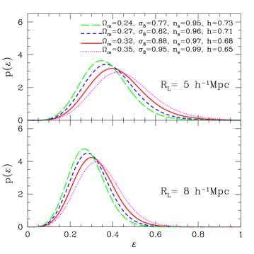
Figure 1: Probability density distributions of the void ellipticity predicted by our analytic model for the four different sets of cosmological parameters at two different smoothing scales: $R_{L}=5$ and $8h^{-1}$Mpc in the upper and the lower panel, respectively. For each case, the void density contrast is set at $\delta_{v}=-0.9$.

Fig. 1 plots $p(\varepsilon)$ at two different Lagrangian scales: $R_{L}=5$ and $8h^{-1}$Mpc in the upper and the lower panel, respectively. Here we assume a $\Lambda$-dominated cold dark matter cosmology ($\Omega_{\Lambda}=1-\Omega_{m}$) and consider four different sets of the key cosmological parameters: $\Omega_{m}$ (matter density parameter), $h$ (dimensionless Hubble parameter), $\sigma_{8}$ (amplitude), and $n_{s}$ (power spectrum slope).

As can be seen, the ellipticity distribution depends quite sensitively on the cosmological parameters. Note that for the cases of low $\Omega_{m}$ and high $h$, voids tend to have more spherical shapes, which in fact can be understood as follows. The void ellipticity distribution is an outcome of the counterbalance between the tidal effect of the dark matter and the expansion of the universe: The tidal effect disturbs the void shapes from spherical symmetry, while the expansion of the universe resists such disturbance.It is also worth noting that the void ellipticity distribution moves toward the low ellipticity as the smoothing scale increases. It indicates that the larger a void is, the more spherical it is.

Numerical Test.—To examine the validity of our analytic model, we test its prediction against the Millennium Run simulation for which the cosmological parameters are specified as $\Omega_{m}=0.25$, $n_{s}=1$, $\sigma_{8}=0.9$ and $h=0.73$ (spr-etal05, ).

In our previous work lee-par06 we have already identified voids in the Millennium Run catalog using the Hoyle-Vogeley (HV02) void-finder algorithm hoy-vog02 . For the detailed description of the void-finding scheme and the properties of the identified voids, see lee-par06 . Among these voids, we select only those voids which contain more than $5$ galaxies. A total of $23652$ voids are found to contain more than $5$ galaxies.

For each selected void, we first calculate the pseudo inertia momentum tensor, $(I_{ij})$, defined as

$$I_{ij}=\frac{1}{N_{vg}}\sum_{\alpha}x^{g}_{\alpha i}x^{g}_{\alpha j},$$ (15)

where $N_{vg}$ is the number of galaxies belonging to a given void, and $(x_{\alpha i}^{g})$ is the position vector of the $\alpha$-th void galaxy. As mentioned in sha-etal06 , the inertia momentum tensor is computed without weighting the position vectors with mass since we are interested in the geometry of voids.

Diagonalizing $(I_{ij})$, we find the three eigenvalues, $I_{1}$, $I_{2}$, and $I_{3}$ (with $I_{1}>I_{2}>I_{3}$), which are related to the semi axis-lengths of a given void as $I_{1}\propto(p_{1}^{2}+p_{2}^{2})$, $I_{2}\propto(p_{1}^{2}+p_{3}^{2})$, $I_{3}\propto(p_{2}^{2}+p_{3}^{2})$ sha-etal06 . Now, the void ellipticity, $\varepsilon\equiv 1-p_{3}/p_{1}$, can be written in terms of $I_{1},I_{2},I_{3}$ as

$$\varepsilon=1-\nu=1-\left(\frac{I_{2}+I_{3}-I_{1}}{I_{1}+I_{2}-I_{3}}\right)^{1/2}.$$ (16)

Measuring $\varepsilon$ of each selected void using Eq. (16), we determine the void ellipticity distribution. Since the distribution depends on the size of void, we divide the whole sample of voids into the four bins according to their effective radius, $R_{E}$, which is defined as $R_{E}\equiv(3\Gamma_{V}/4\pi)^{1/3}$ where $\Gamma_{V}$ is the total volume of a void measured by the Monte-Carlo method devised by hoy-vog02 . Each bin is chosen to include equal number of voids. The range of $R_{E}$, the mean values of $R_{E}$, $\delta_{v}$, and $\varepsilon$ for the four bins are listed in Table  1.

Table 1: The range of the effective radius ($R_{\textrm{E}}^{\textrm{min}}$ and $R_{\textrm{E}}^{\textrm{max}}$), the mean effective radius ($\bar{R}_{\textrm{E}}$), the mean density ($\bar{\delta}_{\textrm{v}}$), the mean ellipticity ($\bar{\varepsilon})$, and the mean number of the galaxies ($\bar{N}_{\textrm{vg}}$) of the voids belonging to the four bins.

	$R_{\textrm{E}}^{\textrm{min}}$	$R_{\textrm{E}}^{\textrm{max}}$	$\bar{R}_{\textrm{E}}$	$\bar{\delta}_{\textrm{v}}$	$\bar{\varepsilon}$	$\bar{N}_{\textrm{vg}}$
$(a)$	$6.42$	$9.04$	$8.37$	$-0.89$	$0.48$	$18$
$(b)$	$9.04$	$10.28$	$9.65$	$-0.89$	$0.43$	$28$
$(c)$	$10.28$	$11.66$	$10.92$	$-0.89$	$0.41$	$39$
$(d)$	$11.66$	$21.52$	$13.00$	$-0.90$	$0.36$	$63$

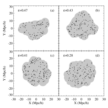
Figure 2: Illustration of the four examples of the voids identified in the Millennium Run simulation. Each panel corresponds to the four bins. The shaded regions and the dots represent the areas of the voids and the positions of the void galaxies in them projected onto the two dimensional plane.

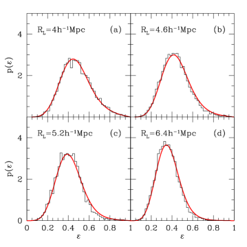
Figure 3: The ellipticity distributions of the voids belonging to the four bins. In each panel the histogram represents the numerical data points from the Millennium Run simulation while the solid line corresponds to the analytic prediction. For the analytic results, the values of the Lagrangian scale radius, $R_{L}$, are evaluated by the relation of $R_{L}=(1+\bar{\delta}_{v})^{1/3}\bar{R}_{E}$.

As shown, $\bar{\varepsilon}$ decreases as the mean $\bar{R}_{E}$ increases. That is, the larger a void is, the more spherical shape it tends to have.

Fig. 2 illustrates the projected images of the four sample voids selected from the four bins, respectively. In each panel the dots represent the positions of the void galaxies and the shaded regions correspond to the areas of the voids. Fig. 3 plots the void ellipticity distributions for the four bins. In each panel, the histogram and the solid line represent the numerical and the analytical results, respectively. For the analytic distribution, the Lagrangian scale radius, $R_{L}$, is given analytically as $R_{L}=(1+\delta_{v})^{1/3}\bar{R}_{E}$. As can be seen the analytic and the numerical results are in excellent quantitative agreements for all cases, proving the validity of our model. It is worth emphasizing here that our model is completely analytical without having any fitting parameter derived from principles. It depends only on the initial cosmological parameters.

Discussion.—The ellipticity distribution of galaxy clusters has been used recently to constrain cosmology jin-sut02 ; lee06 ; ho-etal06 . For the case of clusters, however, the ellipticity distribution cannot be evaluated analytically from the initial conditions because the nonlinear clustering process tends to modify the cluster ellipticities significantly in the subsequent evolution. Although lee-etal05 attempted to derive an analytic fitting model for the cluster ellipticity distribution, their model was shown to be not in good quantitative agreements with the numerical results.

In contrast, we have for the first time shown here that the void ellipticity distribution can be evaluated fully analytically using physical principles and thus be a better indicator of the initial conditions of the universe since the void ellipticities are less vulnerable to nonlinear modifications. By applying our analytic model to real data that will be available from future large galaxy surveys , it may be possible to constrain the cosmological parameters precisely in an independently way.

It is, however, worth nothing that the Hoyle-Vogeley algorithm works very well if a void is found as a spherical low-density region. Nevertheless, we expect that our numerical result would not change sensitively with respect to the void-finding algorithm, given the fact that the ellipticity of a void here is defined in terms of the spatial distribution of galaxies that make up the void but not by the boundary shape of a void.

The Millennium Run simulation used in this paper was carried out by the Virgo Supercomputing Consortium at the Computing Centre of the Max-Planck Society in Garching. We thank the referee and V. Springel for useful comment. This work was supported by the New Faculty Settlement fund of the Seoul National University.

References

- (1) Colless et al., Mon. Not. R. Astron. Soc. 328, 1039 (2001)
- (2) F. Hoyle, and M. S. Vogeley, Astrophys. J. 607, 751 (2004)
- (3) V. Icke, Mon. Not. R. Astron. Soc. 206, 1P (1984)
- (4) J. Dubinski, L. N. da Costa, D. S. Goldwirth, M. Lecar, and T. Piran, Astrophys. J. 410, 458 (1993)
- (5) Van de Weygaert, R., and Van Kampen, E., Mon. Not. R. Astron. Soc. 263, 481 (1993)
- (6) R. K. Sheth, and R. van de Weygaert, Mon. Not. R. Astron. Soc. 350, 517 (2004)
- (7) S. F. Shandarin, J. V. Sheth, and V. Sahni, Mon. Not. R. Astron. Soc. 353, 162 (2004)
- (8) S. F. Shandarin, H. A. Feldman, K. Heitmann, and S. Habib, Mon. Not. R. Astron. Soc. 367, 1629 (2006)
- (9) J. Lee, and D. Park, Astrophys. J. 652, 1 (2006)
- (10) Ya. B. Zel’dovich, Astrophys. & Astron. 5, 84 (1970)
- (11) A. G. Doroshkevich, Astrofizika, 3, 175 (1970)
- (12) J. M. Bardeen, J. R. Bond, N. K. Kaiser, and A. S. Szalay, Astrophys. J. 304, 15 (1986)
- (13) J. Lee, Y. Jing, and Y. Suto, Astrophys. J. 632, 706 (2005)
- (14) V. Springel et al., Nature, 435, 629 (2005). The semianalytic galaxy catalogue is publicly available at http://www.mpa-garching.mpg.de/galform/agnpaper
- (15) F. Hoyle, and M. S. Vogeley, Astrophys. J. 566, 641 (2002)
- (16) Y. Jing, and Y. Suto, Astrophys. J. 574, 538 (2002)
- (17) J. Lee, Astrophys. J. 643, 724 (2006)
- (18) Ho. Shirley, Bahcall, N. A., and P. Bode, Astrophys. J. 647, 8 (2006)