Models of Polarized Light from Oceans and Atmospheres of Earth-like Extrasolar Planets

Abstract

Specularly reflected light, or glint, from an ocean surface may provide a useful observational tool for studying extrasolar terrestrial planets. Detection of sea-surface glints would differentiate ocean-bearing terrestrial planets, i.e. those similar to Earth, from other terrestrial extrasolar planets. Sea-surface glints are localized and linearly polarized. The brightness and degree of polarization of both sea-surface glints and atmospheric Rayleigh scattering are strong functions of the phase angle of the extrasolar planet. The difference of the two orthogonal linearly polarized reflectances may be an important observational signature of Rayleigh scattering or glint. The difference attributable to Rayleigh scattering peaks near quadrature, i.e. near maximum elongation of a circular orbit. The difference attributable to glint peaks at crescent phase, and in crescent phase the total (unpolarized) reflectance of the glint is also near maximum. We present analytic and physical models of sea-surface glints. We modify analytic expressions for the bi-directional reflectances previously validated by satellite imagery of the Earth to account for the fractional linear polarization of sea-surface reflections and of Rayleigh scattering in the atmosphere. We compare our models with Earth’s total visual light and degree of linear polarization as observed in the ashen light of the Moon, or Earthshine. We predict the spatially-integrated reflected light and its degree of polarization as functions of the diurnal cycle and orbital phase of Earth and Earth-like planets of various imagined types. The difference in polarized reflectances of Earth-like planets may increase greatly the detectability of such planets in the glare of their host star. Finally, sea-surface glints potentially may provide a practical means to map the boundaries between oceans and continents on extrasolar planets.

1 Introduction

Terrestrial extrasolar planets have captured the human imagination for much of history. Missions such as Kepler will search for planets in the so-called “habitable zone,” in which the planet may support water in its liquid state (Borucki et al. 2006). The proximity of accomplishing the goal of detecting terrestrial planets, especially in relatively large numbers, begs the question, “What next?” One purpose of this paper is to inform the answer to that question.

We consider the next important goal could be to identify extrasolar planets that not only could support liquid water based upon their size, mass, and proximity to their star, but also indeed demonstrably do have liquid on their surfaces, i.e. oceans, and do have atmospheres of non-negligible column density. Both oceans and atmospheres polarize light reflected from them. In this paper we examine linear polarization as a potentially useful signature of oceans and atmospheres of Earth-like extrasolar planets.

Some of the concepts in this paper have been described independently by others. Hough & Lucas (2003) and Stam, Hovenier, & Waters (2004) noted the efficacy of polarization to reduce the glare of a nearly unpolarized star compared to the Rayleigh-scattered polarized light of a hot Jupiter. Seager et al. (2000), Saar & Seager (2003), and Stam & Hovenier (2005) examined the Rayleigh-scattered light of a hot Jupiter in greater detail. Williams & Gaidos (2004) and Gaidos et al. (2006) examined the unpolarized variability of the sea-surface glint from an Earth-like extrasolar planet, and Williams (2006) has proposed that a satellite of a extrasolar gas giant planet could be brighter than the planet itself due to the much lower albedo of the planet than that of the satellite. Stam & Hovenier (2006) independently examined the observability of the polarized signatures of an Earth-like extrasolar planet, including Rayleigh scattering and sea-surface glint. Schneider (2006) had similar ideas.

Kuchner (2003) and Léger et al. (2004) have proposed that “ocean planets” may form from ice planets that migrate inward and melt; the surfaces of these planets would be liquid water exclusively, i.e. no continents. Although Kuchner expects the liquid surface to be entirely obscured by a thick steam atmosphere, Léger et al. model a liquid ocean under either an obscuring cloud or a clear atmosphere. In the former case, the specular reflection from the ocean would not be visible, and the evidence of liquid water would be indirect: the mean density could be inferred from transits and radial velocities, and the surface temperature could be inferred from the star’s incident flux and the planet’s albedo or from the planet’s infrared emissivity.

In this paper, we explore the potential observational signature of a liquid, especially water, on a planet’s surface: the polarized glint. The observational signatures of glints may be detectable in the orbital phase-dependent and time-dependent spatially-integrated reflected light of the extrasolar planet. The phase dependency of the polarization may allow future astronomers to infer a specularly reflecting surface, and (less reliably) to measure the index of refraction of the medium, n, and if n $\sim\ 1.3$ then that might give some credence to speculation that the medium is liquid water. However, remote sensing of distant worlds generally will admit many possible interpretations, as the following example of Titan illustrates.

West et al. (2005) interpreted the apparent lack of near-infrared specular reflection from Titan, combined with the specular signatures from Earth-based radar as evidence for no liquid oceans on its surface at the locations they studied, circling Titan at ${\sim}-30$° latitude. Liquid lakes have been detected on Titan by observations of the Cassini orbiter, at latitudes north of $+70$° (Mitchell et al. 2006). In general, a lack of a glint cannot prove that liquids do not exist anywhere on an extrasolar planet’s surface. The example of Titan also shows that a glint is not necessarily indicative of liquid water.

Neither radar nor highly spatially-resolved planetary images, such as those of Titan, will be available for extrasolar planets. However extrasolar planets could exhibit a wide range of phase angles, an impossibility for Earth-based observations of the outer planets. For example, using the phase dependency of polarization, Horak (1950) showed the fractional polarization of Venus’ atmosphere is not large and is not due to Rayleigh scattering.

In Section 2 we analyze physical models of specularly reflecting spheres. In Section 3 we modify bi-directional reflectances to account for linear polarization from two mechanisms: Rayleigh-scattering and specular reflection. In Section 4 we model Earth-like planets and demonstrate that the rotation of a planet with surface features such as continents and oceans should modulate the polarized reflectances in a simple and predictable manner. We also simulate the modulation of the polarized reflectances due to orbital phase. Section 5 compares our models with observations of Earthshine. Section 6 discusses the technique of using the glint as a tool for mapping extrasolar planets and estimates the glint’s observability with near-future instrumentation.

2 Observations and Analysis of a Simple Orrery

We constructed simple physical models of planets with uniform surfaces and no atmospheres. The models are 2.5-inch diameter wooden spheres covered uniformly with acrylic paint. Sphere A is painted flat white; sphere B, flat white with a shiny transparent acrylic overcoat; and sphere C, flat black with an identical overcoat. The acrylic overcoats of spheres B and C specularly reflect the incident light. Sphere C is meant to model a deep ocean, because it has a very low albedo for light that is not specularly reflected from the first air-acrylic interface. Sphere B could represent the surface of a planet with a very shallow, sandy ocean, or a mix of ice and water. Each sphere is suspended in a dark room by a wooden dowel, 23 inches (58 cm) from a incandescent filament covered by a 1/4-inch (6-mm) diameter, white, translucent plastic dowel that makes the lamp’s radiance isotropic azimuthally, i.e. in the plane defined by the lamp, the sphere, and the camera. That plane is the plane of incidence for specularly reflected rays, and by convention, the electric field of the s-component is perpendicular ($\perp$) to that plane, and the electric field of the p-component is parallel ($\parallel$) to the plane of incidence. Each sphere was photographed with a quantitative digital camera at angles corresponding to “orbital” phase of 30°, 50°, 70°, 90°, 110°, 130°, and 150°. At each phase angle, four pairs of exposures were taken of each sphere at four angles (0°, 45°, 90°, and 135°) of a linear polarizer in front of the digital camera’s lens. At 0° orientation, the polarizer transmitted the p-component and at 90° it transmitted the s-component.

Even in an otherwise darkened room the light from the lamp illuminates the walls, floor, and ceiling of the room which then illuminate the model “planet.” The latter illumination is undesirable because no such illumination occurs for a real planet. To compensate, we took matched exposure pairs: one with and one without an occulting sphere placed between the “planet” and its “star.” By subtracting the image of the planet in “eclipse” from that of it illuminated directly, we effectively removed the unwanted, indirect illumination.

The spheres can be modeled as a Lambertian surface of albedo A with or without a specular reflection component superposed. The phase angle $\gamma$ is defined to be the angle separating the illuminator and the detector measured from the center of the sphere. The phase function of the integrated light for a Lambertian sphere is (Russell 1916),

$$I(\gamma)={A\over\pi}(sin\gamma+(\pi-\gamma)cos\gamma),$$ (1)

which is normalized such that $I(\gamma=0)=A$, i.e. the results are normalized to full phase and are proportional to the albedo A. With a consistent normalization, the phase function for a sphere with a perfect specularly reflecting surface is (Tousey 1957)

$$I(\gamma)={1\over 4}\times{3\over 2}={3\over 8}.$$ (2)

Thus, the phase function for the specular reflectance from a sphere is

$$I(\gamma)={3\over 8}r,$$ (3)

where r is a linear combination of the Fresnel reflection coefficients,

$$r_{s}={{sin^{2}(\theta_{i}-\theta_{t})}\over{sin^{2}(\theta_{i}+\theta_{t})}}$$ (4)

and

$$r_{p}={{tan^{2}(\theta_{i}-\theta_{t})}\over{tan^{2}(\theta_{i}+\theta_{t})}},$$ (5)

where the angle of incidence $\theta_{i}=\gamma/2$, and according to Snell’s law, $nsin\theta_{t}=sin\theta_{i}$, in which n is the refractive index of the transmissive medium and $\theta_{t}$ is the angle of the transmitted ray. The appropriate linear combination depends on the orientation of the linear polarizer in front of the lens of the digital camera.

Sphere A’s “flat” painted surface is a good approximation to a Lambertian surface. Sphere B’s phase function is approximately that of a Lambertian sphere with a specular-reflection component superposed. The phase functions for spheres A and B are not shown because each is nearly as expected analytically from Equations 1, 3, 4, and 5.

Because one purpose of this paper is to examine the specular reflectance from an ocean that absorbs all the light transmitted below its surface, we compare the observed and theoretical phase functions of sphere C, which is painted flat black with a shiny transparent acrylic overcoat (Figure 1 and Section 4.3). The glint contributes significantly to the spatially integrated light from sphere C at all phase angles and creates the large ratio of one linearly polarized reflectances to the other at phases corresponding to the Brewster angle of incidence. Because the indices of refraction for acrylic and water are 1.50 and 1.33 respectively, the phase angles $\gamma_{B}$ of the theoretical nulls of the p-component are 112.6° and 106.1°, which are double the respective Brewster angles, 56.3° and 53.1°, respectively. For our painted spheres, the observed phase functions are approximately as predicted by Eq. 3, although the p-component of the specular reflectance is larger than predicted, and the s-component is smaller than predicted.

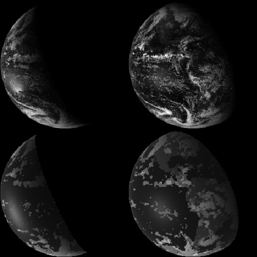
Figure 4: Images from the geostationary satellite GOES EAST (above) taken in unpolarized light on Dec 28, 2005 at 23h45m UTC (left) and 20h45m (right) and corresponding numerical models for the same (below). The phase angle $\gamma=100$° (left) and 59° (right). The sea-surface glint is the bright (white) patch to the lower-left of center of the Earth. The Americas are visible in the image and model at right.

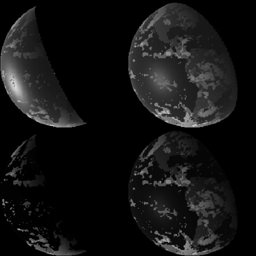
Figure 5: Models images of the scenes from Figure 4 are shown for linear polarized components of light ($\perp$ or s-component above; $\parallel$ or p-component below).

A simple physical model such as sphere C is useful to understand the optical characteristics of specular reflection from a sphere (Figures 1-5): 1) the mean reflectance increases with angle of incidence, 2) the Brewster angle occurs near maximum elongation of a circular orbit, 3) the difference between the polarized reflectances is large for nearly all the “crescent” phases, $\gamma\gtrsim 90$°, and 4) the glint elongates spatially at large angles of incidence. We constructed the physical models in part to validate our numerical models. Similar models could provide opportunities for teaching and outreach at many levels of sophistication, from elementary school to graduate school.

The painted spheres do not model the atmospheric extinction. To account for extinction in a cloudless, Earth-like atmosphere, we multiply the reflectance of Equation 3 (and Figure 2) by an optical opacity,

$$I^{\prime}(\gamma)=I(\gamma)e^{-0.1(sec\ \zeta_{s}+sec\ \zeta_{o})},$$ (6)

where $\zeta_{s}$ and $\zeta_{o}$ are the zenith angles of the star and the observer, respectively, at the point of specular reflection toward the observer (Figure 3). At the point of specular reflection, the star’s zenith angle $\zeta_{s}$ equals the angle of incidence $\theta_{i}$, which equals the angle of reflection, so the airmasses are equal, $sec\zeta_{s}=sec\zeta_{o}$. The extinction coefficient, 0.1, is appropriate for broadband visible light with a solar spectrum (Hayes & Latham 1975). Much of the extinction in a clear atmosphere is due to scattering, not absorption. For astronomical photometry of a star, whether light is lost to absorption or scattering is immaterial. In the case of glint from an ocean, by reciprocity, a similar circumstance applies to the upwelling light (i.e. after reflection from the surface), traveling from the planet’s surface to the observer: scattered light is lost as effectively as absorbed light. The same is true of downwelling light that is scattered upward. However, downwelling light that is forward scattered (downward) may still contribute to the glint, because it may specularly reflect to the observer from a different facet of another wave on the ocean’s surface. In our approximation, we have neglected that effect: scattered light is not permitted to reflect. We have neglected also the interaction of the polarization states of the scattered and specularly reflected light.

3 Analytic Approximations for Polarized Bi-directional Reflectances

We use the analytic bi-directional reflectances of Manalo-Smith et al. (1998, hereafter Paper 1) for visible light, as calibrated from various scene types observed by satellites. We modified the bi-directional reflectances to account for the fractional polarization of Rayleigh scattering in the clear atmosphere and of sea-surface specular reflection. The fractional polarization $p$ is defined from the intensities of the two orthogonal, linearly polarized components,

$$p={{I_{s}-I_{p}}\over{I_{s}+I_{p}}}.$$ (7)

3.1 Rayleigh Scattering

For Rayleigh scattering the two components are

$$I_{s}=k\times 1$$ (8)

and

$$I_{p}=k\times cos^{2}\gamma$$ (9)

where k is independent of $\gamma$ (Lang 1999). Hence, the fractional polarization of Rayleigh scattering is

$$p_{Ray}={{sin^{2}\gamma}\over{1+cos^{2}\gamma}}.$$ (10)

The polarized bi-directional reflectance attributable to Rayleigh scattering is

$$r_{Ray}=C_{2}{{1+cos^{2}\gamma}\over{(uu_{0})^{C_{3}}}}\ {{1\pm p_{Ray}}\over{2}}$$ (11)

where $C_{2}$ and $C_{3}$ are coefficients determined by analysis of Earth Radiation Budget Experiment (ERBE) satellite data and $u$ and $u_{0}$ are direction cosines (see Paper 1). The last term in Equation 11, $(1\pm p_{Ray})/2$ partitions the unpolarized reflectance from Paper 1 into its two polarized reflectances.

For low optical thickness, low surface albedo, and moderate single-scattering optical depth, the degree of polarization $p_{Ray}$ of a Rayleigh scattered atmosphere is nearly unity at phase angle $\gamma=90$°, and tapers to zero at phase angles 0° and 180°. Kattawar & Adams (1971) and Viik (1990) have generalized that result for various optical thicknesses and surface albedos. Because we use a single-scattering model for analytic simplicity, our models may over-estimate the fractional polarization due to Rayleigh scattering. Multiple scattering would be more physically realistic and tend to depolarize the emergent light by a few per cent (e.g. Stam & Hovenier 2005). However, the fractional polarization predicted by the approximations in this paper should not be considered as upper limits, simply because less (or more) cloud cover on an extrasolar planet will increase (or decrease) its net polarization.

In the single-scattering Rayleigh model, the fractional polarization $p_{Ray}$ is independent of wavelength, for wavelengths much larger than the size of the scattering particles. However, as Wolstencroft & Breon (2005) have noted, the fractional polarization of the spatially-integrated light of an Earth-like planet should decrease with increasing optical wavelength due to the strong wavelength dependence ($\lambda^{-4}$) of the Rayleigh-scattering cross section (Jackson 1975) and the flat spectrum of clouds. Dollfus (1957) observed that the polarization of the Earthshine decreased with increasing wavelength: p = 8.4%, 5.4%, and 3.5% at $\lambda$ = 0.49 $\rm{\mu}m$, 0.55 $\rm{\mu}m$, and 0.63 $\rm{\mu}m$, respectively. Wolstencroft & Breon (2005) predict fractional polarization of the Earth’s light at $\lambda=0.443$ $\rm{\mu}m$ and at phase angle $\gamma=90$° to be 20% to 28%, or 0.5 to 0.7 times Dollfus’ estimate or our own (both 40%; Section 5).

The radiances of the clear daytime sky and of Earthshine (Woolf et al. 2002) both decrease with increasing wavelength. In each case, the cause is attributed to atmospheric Rayleigh scattering, which is diluted by the flat spectrum of clouds, causing the Earth to appear, in the words of Sagan (1994), as a “Pale Blue Dot.”

The radiance of the Rayleigh scattering in our model should be proportional to $C_{2}(\lambda/\lambda_{eff})^{-4}$, where $\lambda_{eff}$ is a wavelength at which the coefficient $C_{2}$ is appropriate. The coefficient $C_{2}$ is derived from observations from ERBE scanning radiometers that have sensitivity over 0.2-3.8 $\mu$m, decreasing gradually with wavelength for $\lambda<1\mu$m (Smith et al. 1986). The ERBE radiometer’s sensitivity to a $\lambda^{-4}$ Rayleigh-scattered blackbody approximation to the solar spectrum peaks at $0.27\mu$m, and the weighted-mean wavelength equals $0.35\mu$m. Modeling the telluric absorption by ozone as transparent ($\lambda>0.35$$\rm{\mu}m$) or opaque ($\lambda<0.35$$\rm{\mu}m$) (see e.g. Hayes & Latham 1975) shifts the weighted mean-wavelength from $0.35\mu$m to $0.47\mu$m. The equivalent weighted-mean wavelength for the human eye’s scotopic response (Wyszecki & Stiles 1982) to Rayleigh-scattered sunlight is $0.49\mu$m. Evidently, the observations of the clear atmosphere by the ERBE radiometers and those by the human eye will be similar, and in Section 5 we compare such observations.

3.2 Specular Reflection

We partition the unpolarized reflectance for specular reflection (again from Paper 1),

$$r_{sp}=C_{4}{{C_{5}-1}\over{(uu_{0})^{1.5}(C_{5}-cos\alpha)^{2}}}\ {{1\pm p_{sp}}\over{2}},$$ (12)

into its two polarized reflectances with the last term, where the polarization of specular reflections from water $p_{sp}$ is determined from Equations 3, 4, 5, and 7. Like Equation 11, the other variables of Equation 12 are discussed in Paper 1, so we do not repeat that discussion for the sake of brevity. In this case, the specular reflection comes from an area on the sphere determined by the distribution of tilts of the air-water interface (waves) (Zeisse 1995; Takashima 1985). If a facet of a wave is to specularly reflect the star’s light to the observer, then the angle of incidence of the specular reflection on that facet should be half the phase angle $\gamma$, as before for the idealized sphere.

4 Numerical Modeling of Earth-like Planets

Using maps of the global cloud cover and ice cover recorded daily at 0h, 6h, 12h, and 18h UTC, we simulated Earth-like cloud patterns in addition to entirely clear atmospheric conditions.

4.1 Comparison to Unpolarized Satellite Observations of Earth

We obtained a map of Earth’s major land covers from the ISLSCP. We converted the ISLSCP land cover classification to ERBE landforms of Paper 1 as follows. We treated ISLSCP “ice” and “tundra” as Paper 1 “snow,” ISLSCP “desert” as Paper 1 “Sahara desert,” and all other ISLSCP land covers as Paper 1 “land.” We interpreted brighter pixels of the SSEC cloud cover maps as indicative of greater cloudiness. Over land we allowed four possibilities: clear, partly cloudy, mostly cloudy, and overcast because those had bi-directional reflectances parameterized in Paper 1. We treated ISLSCP “water” as Paper 1 “ocean,” either the Dlhopolsky & Cess (1993) clear ocean model or the mostly cloudy ocean or overcast as appropriate for the brightness of the cloud cover map at each particular location. We did not allow for partly cloudy conditions over oceans simply because to do so would have required introducing another parameter, the degree of partial cloudiness.

It is worth noting that the specific details of land forms, cloud cover, etc of our model Earth need not be authentic to be useful, because other worlds will not be identical to Earth. On the other hand, the fidelity of our Earth model in reproducing observations of the Earth (Figure 4) does contribute to our confidence in the model’s predictive accuracy for potential observations of Earth-like extra-solar planets.

4.2 Planets with Earth-like Oceans and Continents: Diurnal Light Curves

That the short-wavelength light curves of the Earth during one diurnal cycle in Figure 1 of Ford, Seager, & Turner (2001, hereafter Paper 2) match ours (Figure 6) confirms the results of Paper 2 and verifies our numerical methods. The diurnal light curve of our model of an Earth with no atmosphere agrees in detail with that of Paper 2 (its Figure 1a). The mean of the two orthogonal linearly polarized reflectances attributable to Rayleigh scattering from a cloud-free Earth-like atmosphere at phase $\gamma=90$° is $\sim$0.02 in the units of Figure 6, independent of diurnal cycle. Figure 6 models the Earth for Sep 22, 2005, viewed from outside the solar system in the direction, (RA,DEC) = (6^h,0°). Zero time corresponds to Julian date 2453636.184. We did not simulate the same cloud pattern as Paper 2 did, so Figure 2 of Paper 2 matches our corresponding diagram only generally: the mean and variation about the mean of the unpolarized reflectance are similar in the two simulations.

In Figure 6 the difference between the s- and p-components of linearly polarized reflectance is anti-correlated with the total reflectance, because clouds increase the total reflectance while attenuating the two mechanisms for polarization, glint from the ocean and Rayleigh scattering of the clear atmosphere. As the Earth rotates, the difference of the s- and p-components is modulated: the local maxima correspond to clear skies over oceans; the local minima, to continents or very cloudy regions. The magnitude of the modulation is approximately one half that expected from a total obscuration (or not) of a idealized spot with a specular reflectance given by 6. We attribute the reduced magnitude of the modulation to partial obscuration of the specularly reflecting ocean by clouds in our simulated images. The region of specular reflection is extended on the globe because the tilts of the facets of waves spreads the angular distribution of the specular reflection, which corresponds to a spatial spread on the globe as observed from space.

4.3 Planets with Uniform Surfaces: Phase-dependent Light Curves

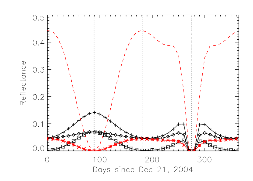
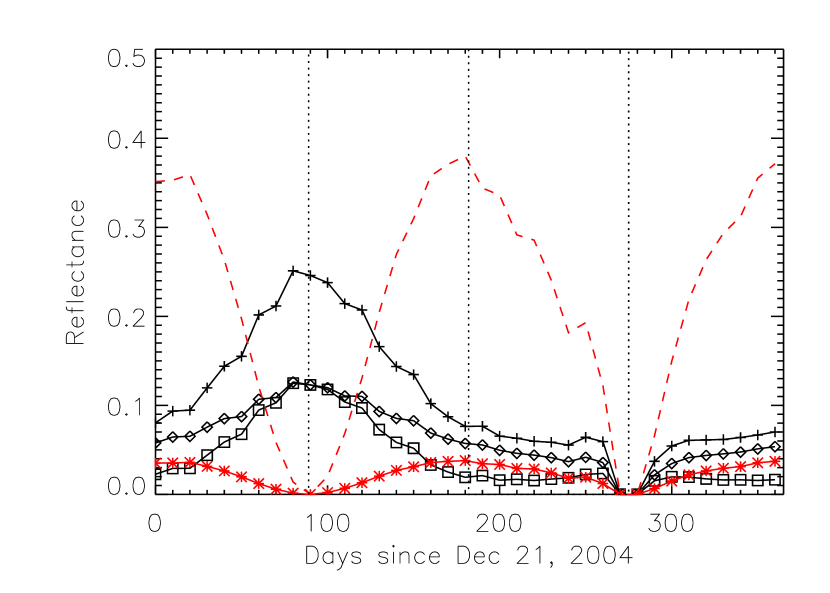
Figure 7: Planet with ocean surface. The reflectance is normalized to that of a Lambertian sphere at its brightest, fully-illuminated phase. The planet’s surface is of a single form, ocean, under an Earth-like atmosphere that is entirely clear (left) or has clouds with Earth-like covering fraction and reflectance (right). The hypothetical observer is located outside the solar system in the ecliptic plane, in the direction of the vernal equinox. Dates corresponding to the planet’s superior conjunction (i.e. full phase), quadrature, and inferior conjunction (i.e. new phase) are indicated by the dotted lines at 89, 182, and 275 days, respectively, after Dec 21, 2004. The reflectance in the two orthogonal linear polarizations, s and p, are indicated by the diamonds and squares, respectively. Also plotted is the sum ($+$ symbols) of the s and p components and their difference (asterisk, in red). For clarity ten times the latter is plotted as a dashed line.

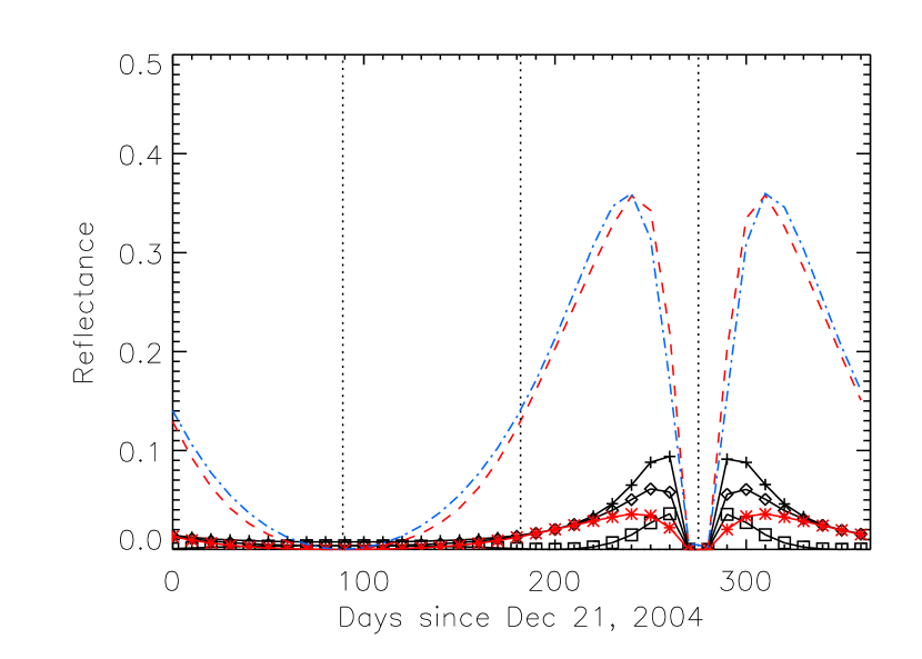
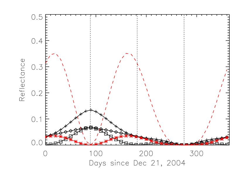
Figure 8: Planet with ocean surface and no clouds. The specular component has been separated from the others and plotted by itself (left) and removed (right) in order to aid interpretation of Figure 7. Legend is the same as Figure 7. The difference of the s- and p- components of linearly polarized reflectance from the simple analytic approximations (Equation 6 and Figure 3) is the dash-dot line in the left diagram. The latter is nearly identical to the equivalent curve generated by numerical integration of the bi-directional reflectances (dashed line).

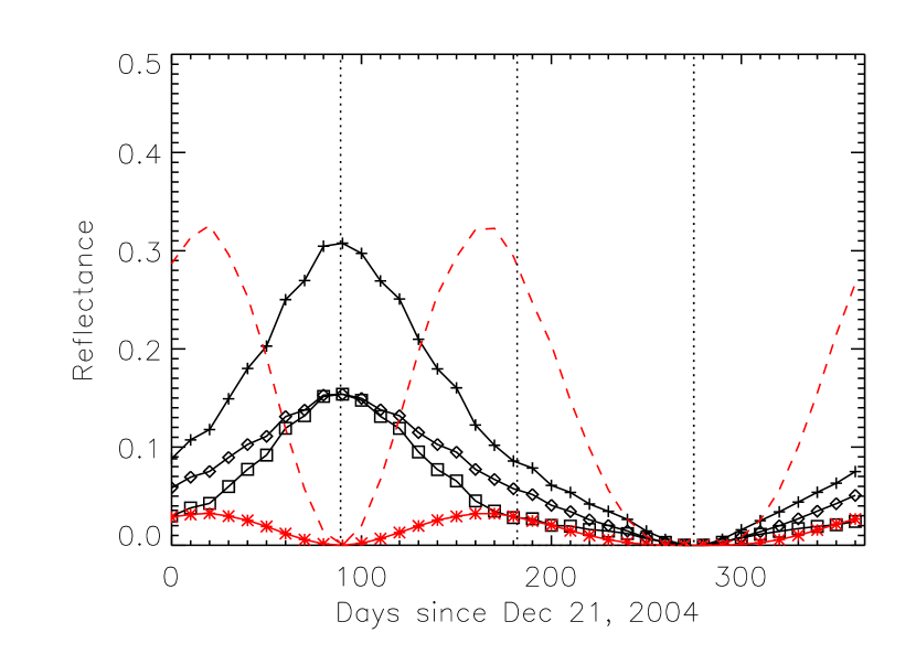
Figure 9: Planet with land surface. Legend is the same as Figure 7.

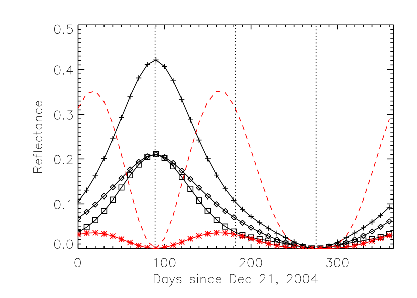
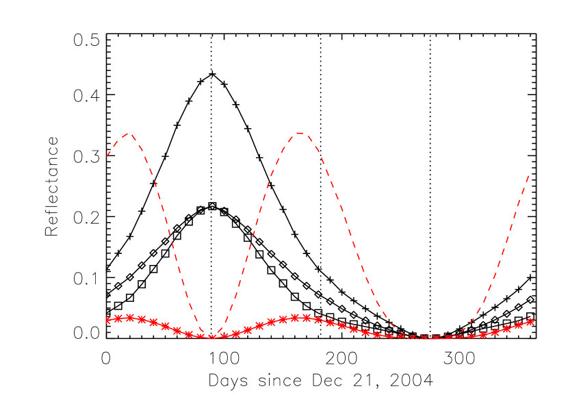
Figure 10: Planet with desert surface. Legend is the same as Figure 7.

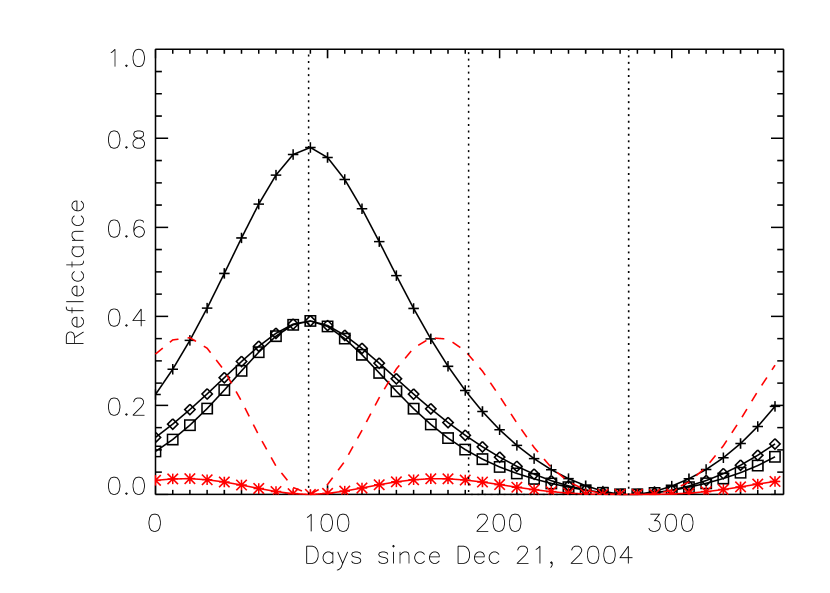
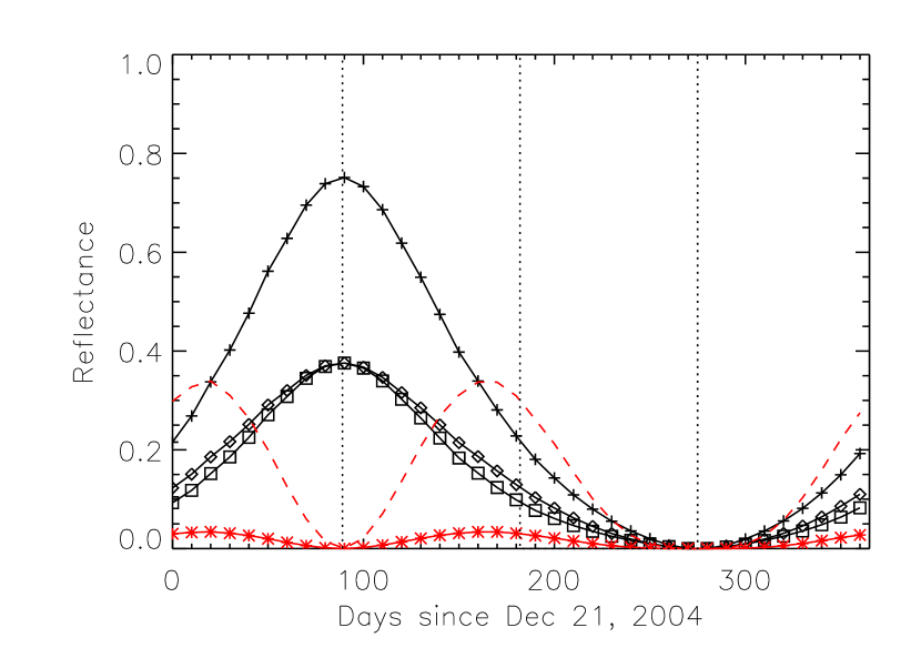
Figure 11: Planet with snow surface. Legend is the same as Figure 7. Due to the large reflectance of snow, the vertical scale is twice that of the others, Figures 7-10.

We simulated planets with uniform ERBE scene types from Paper 1 of ocean, land, desert, and snow, with or without Earth-like clouds for one year beginning on Dec 21, 2004 (Figures 7 - 12). Representing the data as functions of days since a specific date, instead of phase, authentically includes the clouds associated with the seasons, although, for the purposes of this paper, such effects are negligible. The phase of the Earth advances at $\sim$1° per day, and specific phases (full, quarter, new) are indicated on the diagrams.

A “water-world” planet with an ocean surface, a clear sky, and no land shows a prominent asymmetry about quarter phase in the difference between the two linear polarizations (Figure 7). Figure 8 shows the asymmetric pattern of the difference is caused by the superposition of specular reflection, which is enhanced at crescent phases, and Rayleigh scattering, which is symmetric about quarter phase. Clouds attenuate the magnitude and the asymmetry of the difference. This magnitude is affected less than the asymmetry, as expected, because in the models of Paper 1, most of the Rayleigh scattering occurs above the clouds, whereas the glint is extinguished wherever there are clouds. In the red and infrared, the specular reflection will persist whereas the Rayleigh scattering will be attenuated by $\lambda^{-4}$. Hence, the two diagrams of Figure 8 can be considered as approximations to models observed in the red (specular only) or with no specularly reflecting ocean (Rayleigh only).

For comparison, Figure 8 includes the difference of the s- and p- components of linearly polarized reflectance from the analytic formulae of Section 2, including atmospheric extinction. The similarity of the phase curve of the difference from the analytic formulae (Equation 6) to that from the numerical simulations (Section 3) is remarkable.

5 Comparison to Earthshine reflected from the Moon

The peak polarization of the Earthshine is $\sim$11% near lunar phase angle 80°, i.e. a slightly gibbous moon, corresponding to Earth’s phase angle 100° (Dollfus 1957). The numerical models described in Section 4.3 predict that the fractional polarization peaks near Earth’s phase angle $\gamma=$ 100°, in agreement with Dollfus’ observations.

The polarization of the Earthshine is less than that of the Earth’s light due to depolarization upon reflection from the Moon (Dollfus 1957). Adjusting Dollfus’ analysis (1957) for a modern value of the Earth’s albedo, A = $0.297\pm\ 0.005$ (Goode et al. 2001), we multiple by four times (4.0) the observed fractional polarization of Earthshine (Dollfus 1957, Fig 25), to obtain the phase-dependent fractional polarization $p(\gamma)$ of the Earth’s light as seen from space. The results for $p(\gamma)$ are plotted as filled circles on Figures 12 by associating each phase $\gamma$ with an appropriate date.

6 Discussion

From Equations 1, 3, 4, and 5, we predict that an idealized planet with no atmosphere and an air-water surface illuminated by unpolarized light will specularly reflect more s-polarized light than a planet of identical size with an unpolarizing Lambertian surface of albedo A, for phase angles, $\gamma>\gamma_{c}$, with $\gamma_{c}=$ 99.2°, 110.6°, 116.4°, 120.3°, and 123.2° for A = 0.2, 0.4, 0.6, 0.8, and 1.0 respectively. The corresponding separations from the star are 99%, 94%, 90%, 86%, and 84% of maximum separation of a circular orbit. Also, the glint’s reflectance in s-polarized light exceeds that of the Lambertian surface for the fraction of a circular orbit, (180°- $\gamma_{c}$)/180° = 45%, 39%, 35%, 33%, and 32%, respectively for the five values of albedo.

In principle wind speed may be inferred from the glitter pattern of specular reflection from sea surface, because as the wind increases, the wave height does also, which increases the tilts of the facets of the waves, which broadens the specular reflection in angle compared to that of a calm, locally flat surface (Zeisse 1995; Henderson, Theiler, & Villeneuve 2003). Cox & Munk (1954) observed an empirical linear relationship between the local wind speed and the mean squared slope of waves on Earth’s oceans. However the relationship depends also on a variety of potential factors such as the fetch and the duration of the wind, currents in the water, and stronger winds (storms) at great distances. That the average wind speed above the surface of an ocean of an extrasolar planet in principle might be measured is worth noting, perhaps, even if it seems entirely impractical at the present time.

The sea-surface glint will increase and decrease in brightness as ocean and land, respectively, rotate into the localized area of potential specular reflection. The small size of the glint area, relative to the radius of the planet, provides a high-resolution technique to image the boundaries between the oceans and the continents, if they exist. In principle, for some combinations of orbital inclination and planetary obliquity, this technique could map the boundaries of continents in two dimensions. Such a map might provide additional evidence of plate tectonics on the extrasolar planet in the manner of the western edge of Africa matching the eastern edge of South America. Although reconstructing the continental boundaries from light curves is beyond the scope of this paper, a one-dimensional example that also includes authentic Earth-like clouds is presented in Figure 6. The oceans and continents are quite apparent in the difference between the two linear polarizations. Temporally and spatially variable clouds will add noise to any reconstruction of underlying surface features. However, we expect reconstructions using the polarized glint could be more robust than those that rely solely on non-specularly reflected light for two reasons: 1) the area of the specular reflection is small compared to the planet’s radius, and 2) the glint is both very bright and strongly polarized, each in a manner predictable from simple optics, whereas other surface features and clouds tend not to be strongly polarized. (The Rayleigh-scattered light is strongly polarized but can be discriminated against by observing in the red, as we have noted previously). By examining the difference of the two orthogonal polarizations over many diurnal cycles, and over a variety of orbital phases, one might be able to ascertain the underlying continental boundaries and the covering fraction of clouds. In general terms, the technique of using the localization of the glint for imaging continental boundaries on extrasolar planets is akin to the method of imaging the reflected light from a collimated laser beam to overcome turbidity in the ocean environment (e.g. Moore et al. 2000).

In order to demonstrate the potential utility of the polarized glint from an Earth-like extrasolar planet, we now estimate its observability. These estimates are purposefully simplistic in order to permit the reader to appreciate the advantages, constraints, and limitations of the proposed technique. Stam & Hovenier (2005) similarly analyzed the observability of Rayleigh scattered light from Jovian planets. For both specular reflection and Rayleigh scattering, the s-component is larger than the p-component, so the two mechanisms add constructively to the linear polarization of an Earth-like planet (Figure 5). However, Rayleigh scattering is most significant at short wavelengths whereas glint is nearly achromatic. Because optical systems tend to perform better at longer wavelengths, there may be advantages to detecting glint instead of Rayleigh-scattered light.

A telescope of collecting efficiency $\epsilon$ and diameter D will collect photons at a rate ${\dot{p}}$ from the specular reflection of light from a sphere of radius R and reflectivity r at distance a from a star emitting photons at rate L at distance d from Earth, where

$$\dot{p}\approx{{\epsilon\pi D^{2}}\over{4}}{{L}\over{4\pi a^{2}}}{{R^{2}\ r}\over{4}}{{1}\over{4\pi d^{2}}}.$$ (13)

The factors of Equation 13 are from left to right, the effective area of the telescope, the star’s (photon) irradiance upon the planet, the specular reflectivity of a sphere (Tousey 1957), and the dilution over the distance to Earth. The photon rate from the star directly on the same telescope is

$$\dot{p}_{*}\approx{{\epsilon\pi D^{2}}\over{4}}{{L}\over{4\pi d^{2}}},$$ (14)

and the ratio of the two photon rates is

$$\dot{p}/\dot{p}_{*}\approx{{R^{2}\ r}\over{4}}{{1}\over{4\pi a^{2}}}.$$ (15)

For nominal values, D = 10 m, $\epsilon=0.5$, L = L_⊙, a = 1 A.U., R = R_e, d = 10 pc, the photon rate $\dot{p}\approx 1.4$ r photons s^-1. For simplicity, we assume that the star emits all of its luminosity at a wavelength near the peak of its spectrum, $\lambda=0.6\mu$m, but the ratio in Equation 15 is independent of that assumption and equals $3.6\times 10^{-11}$ times r for the nominal parameters.

In this paragraph, we assume that the planet is observed such that its glint is much brighter in one polarization than the other, i.e. at a phase angle $\gamma\gtrsim 90$°. For an air-water interface, the peak difference of the reflectivities of the two linear polarizations is $\sim 10$%, i.e. r $\sim 0.1$ (Figure 3), which can be substituted into Equation 13 to estimate the excess photon rate in one polarization compared to the other. The unpolarized component of the planet’s light is negligible with respect to the star’s light scattered in the optics or Earth’s atmosphere. For the nominal parameters above, the angle between the planet and the star, a/d, is approximately eight times larger than the diffraction width for the telescope, $\lambda$/D. For sake of discussion, we assume a coronagraph that can suppress the diffracted star’s light at $\sim 8\lambda$/D by the factor $\sim 10^{-6}$ with respect to the on-axis image of a point source. That is $\sim 10^{-2}$ times the local maximum of an Airy pattern at that separation, and is approximately the geometric mean between demonstrated performance with ground-based adaptive optics ($\sim 10^{-4}$, Hinkley et al. 2006) and laboratory conditions in a moderately wide spectral bandpass ($\sim 10^{-8}$, Trauger et al. 2004). By simultaneously forming two orthogonal, linearly polarized images, or with an equivalent technique, one may design the two residual speckle (or diffraction) patterns to be nearly identical and thus to subtract nearly as well as permitted by Poisson statistics (however, for technical challenges, see Carson et al. (2006)). If an imaging polarimeter capable of detecting a fractional polarization of $\sim 10^{-5}$ could be placed in series with the coronagraph, then the polarized glint from the an Earth-like planet would be nearly detectable, if the stellar and instrumental polarizations can be eliminated by design or by analysis. With respect to the nominal values, if the planet is twice as large, and twice as near to its star, the planet-to-star flux ratio would be $0.6\times 10^{-10}$, or $2^{4}=16$ times larger than nominal, i.e. $\sim 6$-$\sigma$ greater than the nominal contrast limit of $10^{-11}$. Because coronagraphs, polarimeters, and telescopes of nearly these characteristics exist already, and perhaps also do such planets (e.g. Lovis et al. 2006), some additional advances may permit detection of oceanic planets around nearby stars (Schmid et al. 2005, 2006).

In this paragraph we assume the planet is observed with superior instrumentation that entirely suppresses the star’s diffracted light at the location of the planet. As derived previously, the photon rate from the planet $\dot{p}\approx 1.4$ r photons s^-1, and r $\approx 0.1$, so $\dot{p}\approx 0.14$ photons s^-1. In an integration time of one hour, a Poisson-limited signal to noise ratio of $\sim$20 is achieved. The size of the glint on an Earth-like planet sets both a spatial and a temporal filter on the technique of imaging via photometry of the glint: it smooths out surface features to $\sim 15$° resolution, corresponding to $\sim 1$ hour of longitude (Figure 6).

One advantage of the polarization of the reflected light is that the two linear components can be measured separately and simultaneously. In that case, the difference can be formed, so that unpolarized light will cancel out. In the case of a speckle pattern, whether it is variable on short timescales, such as that of an adaptive optics system, or not, such as that of an optical system in space, it may be difficult to determine the sum of the two polarized components from only the planet even in cases where the difference of the two components is detected well. In that circumstance, we may measure the difference only and will be unable to determine the fractional polarization of the planet. For this reason, we emphasize the difference of the two components in this work.

7 Summary and Future Work

This paper predicts the spatially-integrated polarized reflectances of the Earth and Earth-like planets by simple analytic formulae and by numerically integrating analytic approximations for the polarized bi-directional reflectances of various scene types. Models with and without Earth-like clouds are compared. Light curves as functions of orbital phase are provided for an Earth-like planet and for terrestrial planets with a variety of homogeneous surface types, again with or without Earth-like clouds. The models predict the it shape of the phase function of the Earthshine’s linear polarization observed by Dollfus (1957); the maximum polarization agrees with Dollfus’ observations but is approximately twice as large as that predicted by Wolstencroft & Breon (2005). Simple estimates of the observability of extrasolar Earth-like planets are provided and indicate that near-future technology may be able to detect such planets by the difference of planetary reflectance in two linear polarizations. Bi-directional reflectances as functions of wavelength would extend the models described here; the POLDER satellite can provide such data for various scene types (Wolstencroft & Breon 2005). We plan to observe the time-variability of the Earth’s polarized glint in the Earthshine to validate the technique of imaging clouds and continental boundaries described in Section 6 and illustrated in Figure 6.

Figure 1: Specular reflectivity of acrylic. Integrated reflectances from a sphere painted flat black with a shiny acrylic overcoat are plotted at each angle in the two orthogonal s- and p-components of linear polarization, upper and lower points respectively. Each middle data point is the mean of the other two. We selected a single scale factor to match the observed mean reflectances to the theoretical curve. The dashed and dotted lines are the s- and p-components respectively, for refractive index n = 1.50 from Equations 4 (dashed) and 5 (dotted), their mean (solid), and their difference (dashed-dotted). The same curves are plotted with respect to angle of incidence (left) and projected separation from the “star,” i.e. the source of illumination (right). In the latter, the separation is normalized to the maximum separation, a circular orbit is assumed, and only points with phase angle $\gamma\geq 110$°, i.e. crescent phase, are plotted, for clarity.

Figure 2: Specular reflectivity of water. Same as Figure 1 except for an index of refraction n = 1.33. No experimental data are plotted.

Figure 3: Specular reflectivity of water, including atmospheric absorption. Same as Figure 2 except reflectivities are attenuated by exp(-0.1($sec\zeta_{s}+sec\zeta_{o}$)), where $sec\zeta_{s}$ and $sec\zeta_{o}$ are the airmasses of the star and the observer, at their respective zenith angles, $\zeta_{s}$ and $\zeta_{o}$, at the point of specular reflection.

Figure 6: Diurnal light curves for the Earth viewed at quadrature. The reflectance is normalized to 1.0 for a full-phase Lambertian sphere. Conditions were selected to match those of Figures 1 and 2 of Paper 2. Our model of the unpolarized reflectance (left, $+$ symbols) of the Earth with its atmosphere removed. The reflectance (right, $+$ symbols) for the same conditions except including the atmosphere and authentic clouds. The dashed line (right) is twice the difference between the s- and p-components of linear polarization. Major surface features at the location where the sea-surface glint is or would be, in the case of continents, are labeled above the dashed line: the local maxima correspond to clear skies over oceans (Pacific, Indian, and Atlantic, as labeled); the local minima, to continents (Africa and South America, as labeled) or cloudy regions (between the Pacific and Indian oceans).

Figure 12: Polarization fractions. Planets of various surfaces are simulated with an Earth-like atmosphere that is entirely clear (upper curves) or has clouds with Earth-like covering fraction and reflectance (lower curves). From left to right and top to bottom, surfaces are ocean, land, desert, snow, an ocean with only its specular reflection, and an ocean with the specular-reflection component eliminated. Filled circles are data scaled from observations of Earthshine (Dollfus 1957).

References

- Alonso et al. (2001) Alonso, L., Moreno, J., & Leroy, M. 2001, ESA SP-499: The Digital Airborne Spectrometer Experiment (DAISEX), 183
- Borucki et al. (2006) Borucki, W. J., et al. 2006, AAS/Division for Planetary Sciences Meeting Abstracts, 38, #45.01
- Bréon et al. (2002) Bréon, F. M., et al. 2002, Advances in Space Research, 30, 2383
- Carson et al. (2006) Carson, J. C., Kern, B. D., Breckinridge, J. B., & Trauger, J. T. 2006, IAU Colloq. 200: Direct Imaging of Exoplanets: Science & Techniques, 441
- Danjon (1954) Danjon, A., The Earth as a Planet, edited by G.P. Kuiper, pp.726-738, University of Chicago Press, 1954
- Dlhopolsky & Cess (1993) Dlhopolsky, R., & Cess, R. D. 1993, J. Geophys. Res., 98, 16713
- Dollfus (1957) Dollfus, A. 1957, Supplements aux Annales d’Astrophysique, 4, 3
- Ford (2006) Ford, E. B., private communication.
- Ford et al. (2001) Ford, E. B., Seager, S., & Turner, E. L. 2001, Nature, 412, 885 (Paper 2)
- Gaidos et al. (2006) Gaidos, E., Moskovitz, N, & Williams, D. M. 2006, IAU Colloq. 200: Direct Imaging of Exoplanets: Science & Techniques, XXX
- Goode et al. (2001) Goode, P. R., Qiu, J., Yurchyshyn, V., Hickey, J., Chu, M.-C., Kolbe, E., Brown, C. T., & Koonin, S. E. 2001, Geophys. Res. Lett., 28, 1671
- Hayes & Latham (1975) Hayes, D. S., & Latham, D. W. 1975, ApJ, 197, 593
- Henderson (2003) Henderson, B. G., Theiler, J. & Villeneuve, P. 2003, Remote Sensing of Environment, 88, 453
- Hinkley et al. (2006) Hinkley, S., et al. 2006, ArXiv Astrophysics e-prints, arXiv:astro-ph/0609337
- Horak (1950) Horak, H. G. 1950, ApJ, 112, 445
- Jackson (1975) Jackson, J. D. 1975, Classical Electrodynamics, New York: Wiley, 2nd ed.
- Kattawar & Adams (1971) Kattawar, G. W., & Adams, C. N. 1971, ApJ, 167, 183
- Kuchner (2003) Kuchner, M. J. 2003, ApJ, 596, L105
- Lang (1999) Lang, K. R. 1999, Astrophysical formulae / K.R. Lang. New York : Springer, 1999. (Astronomy and astrophysics library,ISSN0941-7834)
- Léger et al. (2004) Léger, A., et al. 2004, Icarus, 169, 499
- Look (1973) Look, D. C. 1973, Appl. Opt., 12, 621
- Lovis et al. (2006) Lovis, C., et al. 2006, Nature, 441, 305
- Manalo-Smith et al. (1998) Manalo-Smith, N., Smith, G. L., Tiwari, S. N., & Staylor, W. F. 1998, J. Geophys. Res., 103, 19733 (Paper 1)
- Miller & Vegh (1993) Miller, A. R. & Vegh, E. 1993, SIAM Review, 35, 472
- Mitchell et al. (2006) Mitchell, K. L., et al. 2006, AAS/Division for Planetary Sciences Meeting Abstracts, 38, #52.05
- Moore et al. (2000) Moore, K.D., Jaffe, J. S., and Ochoa, B. L. 2000, Journal of Atmospheric and Oceanic Tech., Vol. 17, No. 8, 1106
- Russell (1916) Russell, H. N. 1916, ApJ, 43, 173
- Saar & Seager (2003) Saar, S. H., & Seager, S. 2003, ASP Conf. Ser. 294: Scientific Frontiers in Research on Extrasolar Planets, 294, 529
- Sagan (1994) Sagan, C. 1994, Pale Blue Dot, New York : Random House, 1st ed.
- Schneider (2006) Schneider, G. 2006, private communication.
- Schmid et al. (2005) Schmid, H. M., et al. 2005, ASP Conf. Ser. 343: Astronomical Polarimetry: Current Status and Future Directions, 343, 89
- Schmid et al. (2006) Schmid, H. M., et al. 2006, IAU Colloq. 200: Direct Imaging of Exoplanets: Science & Techniques, 165
- Seager et al. (2000) Seager, S., Whitney, B. A., & Sasselov, D. D. 2000, ApJ, 540, 504
- Stam et al. (2006) Stam, D. M., de Rooij, W. A., Cornet, G., & Hovenier, J. W. 2006, A&A, 452, 669
- Stam & Hovenier (2005) Stam, D. M., & Hovenier, J. W. 2005, A&A, 444, 275
- Stam & Hovenier (2006) Stam, D. M. & Hovenier, J. W. 2006, IAU Colloq. 200: Direct Imaging of Exoplanets: Science & Techniques, XXX
- Stam et al. (2004) Stam, D. M., Hovenier, J. W., & Waters, L. B. F. M. 2004, A&A, 428, 663
- Takashima (1985) Takashima, T. 1985, Earth Moon and Planets, 33, 59
- Taylor & Stowe (1984) Taylor, V. R., & Stowe, L. L. 1984, J. Geophys. Res., 89, 4987
- Todd (1959) Todd, E. P. 1959, Journal of the Optical Society of America (1917-1983), 49, 491
- Tousey (1957) Tousey, R. 1957, Journal of the Optical Society of America (1917-1983), 47, 261
- Trauger et al. (2004) Trauger, J. T., et al. 2004, Proc. SPIE, 5487, 1330
- Viik (1990) Viik, T. 1990, Earth Moon and Planets, 48, 41
- West et al. (2005) West, R. A., Brown, M. E., Salinas, S. V., Bouchez, A. H., & Roe, H. G. 2005, Nature, 436, 670
- Williams (2006) Williams, D. M. 2006, private communication.
- Williams & Gaidos (2004) Williams, D. M., & Gaidos, E. 2004, Bulletin of the American Astronomical Society, 36, 1173
- Williams & Knacke (2004) Williams, D. M., & Knacke, R. F. 2004, Astrobiology, 4, 400
- Wolstencroft & Breon (2005) Wolstencroft, R. D., & Breon, F.-M. 2005, Astronomical Society of the Pacific Conference Series, 343, 211
- Woolf et al. (2002) Woolf, N. J., Smith, P. S., Traub, W. A., & Jucks, K. W. 2002, ApJ, 574, 430
- Wyszecki & Stiles (1982) Wyszecki, G., & Stiles, W. S. (1982). Color Science: concepts and methods, quantitative data and formulae. (2nd ed.). New York: Wiley.
- Zeisse (1995) Zeisse, C. R. 1995, Journal of the Optical Society of America A, 12, 2022