Simulation of up- and down-going neutrino induced showers at the site of the Pierre Auger Observatory

Abstract

We present a study about the possibility to detect neutrino induced extensive air showers at the Pierre Auger Observatory. The Monte Carlo simulations performed take into account the details of the neutrino propagation inside the Earth, the air as well as the surrounding mountains which are modelled by a digital elevation map. Details on the sensitivity with respect to the incoming direction as well as the aperture and the total observable event rates are calculated on the basis of various assumptions of the incoming neutrino flux.

I Introduction

The detection of very high energy cosmic neutrinos, above 1 EeV, is important as it may allow to identify the most powerful sources in the Universe.

In the first place, neutrinos, due to their small cross-section can travel cosmological distances without interactions. Hence they might carry astrophysical information about their sources which are commonly believed to be optically thick [1].

Second, due to their connection to the emission of cosmic nuclei and gamma rays, they might help to solve the problem of the origin of ultra high energy cosmic rays (UHECRs). In fact although the existence of UHECRs is experimentally proven, their composition and origin are still unknown. Many models have been proposed to explain the origin of UHECRs. Some of these, which involve mechanisms of particle acceleration (bottom-up), claim that they might be produced by Active Galactic Nuclei (AGN) and Gamma Ray Bursts (GRB) [2]. In such scenarios neutrinos could be produced with an upper flux limit given by the Waxman-Bahcall (WB) bound [1]. Other models claim that UHECRs might come from the decay of super-massive objects (top-down): These objects are expected to be produced by radiation, interaction or collapse of topological defects such as monopoles, cosmic strings, etc. [3]. The topological defect models predict a larger flux of photons and neutrinos arriving at Earth than the bottom-up models. Finally, high energy neutrinos could be also produced through pion decay when protons interact with the cosmic microwave background. These neutrinos are so-called cosmogenic neutrinos [4].

Nevertheless, due to their vacuum oscillations [5], a flux of high energy cosmic neutrinos is expected to be almost equally distributed among the three neutrino flavours. Therefore the study of oscillation effects on high energy neutrino fluxes can be used to study the neutrino mixing and distinguish amongst different mass schemes.

According to the models described above, a low incoming flux of neutrinos is expected. In addition, neutrinos have a small interaction probability. Therefore, in order to get a detectable rate, very large neutrino detectors are needed such as the Pierre Auger Observatory [6]. In particular, for Auger Observatory Earth-skimming $\nu_{\tau}$ showers are the best suited candidates to produce detectable showers. Studies of such possibilities were recently presented in Refs. [7, 8, 9, 10, 11].

In this paper to exemplify the potential and the features of the developed simulation tool we study neutrino induced extensive air showers (EAS) focusing on the fluorescence detector (FD) set up at the Pierre Auger Observatory. Taking into account the details of the neutrino propagation inside the Earth and in the Atmosphere as well as the topography of the Pierre Auger Observatory site, the directional dependence of the neutrino rate for up-going and down-going neutrino showers (probability maps) are evaluated accounting for the 10% duty cycle for the FD. The WB bound is used as an initial neutrino flux. We use the ellipsoidal model of the Earth based on the so-called datum WGS84 [12] model. In addition, we use an elevation map of the mountains surrounding the Auger site. We find that the shape of the surrounding area influences significantly the calculated neutrino rates. To investigate the response of the FD for up-going showers, we generate the longitudinal profiles of shower development using the EAS MC generator AIRES [13]. The light propagation and the hardware detector trigger are simulated by means of the Auger software framework called Offline [14]. Finally the aperture, acceptance and neutrino rate are calculated for up-going $\nu_{\tau}$ showers.

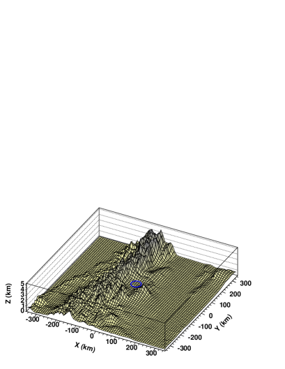
Figure 1: Topography of the Auger site according to CGIAR-CSI data. The centre of the map corresponds to the centre of the Auger array (latitude $\phi_{Auger\_center}=35.25^{\circ}$ S, longitude $\lambda_{Auger\_center}=69.25^{\circ}$ W). The Auger position is marked by a circle.

II Method

The software tool used in the present paper is based on the code ANIS (All Neutrino Interaction Simulation) [15]. ANIS is a code originally developed by A. Gazizov and M. P. Kowalski for the complete simulation chain of neutrino propagation and interaction in the context of the AMANDA experiment [16]. It allows to generate $\nu$-events of all flavours, to propagate them through the Earth and finally to simulate $\nu-$interactions within a specified volume inside the Earth. All relevant Standard Model processes (charged current (CC), neutral current (NC) $\nu N$-interactions and resonant $\bar{\nu}_{e}-e^{-}$ scattering) are implemented. In addition, neutrino regeneration at all orders is included. The density profile of the Earth is chosen according to the Preliminary Earth Model [17]. Deep inelastic $\nu-N$-cross-sections are calculated from Quantum Cromo Dynamics (pQCD) with structure functions according to CTEQ5 [18] and with a logarithmic extension into the small-x region. The tau decay is simulated using the program TAUOLA [19]. In order to simulate neutrino showers suitable to be detected by the Pierre Auger Observatory, some important changes and extensions of the code were needed. For instance, in ANIS neutrino propagation and tau decay are simulated only inside the Earth. Instead, we need to simulate also the propagation through the atmosphere. Moreover, it is necessary to take into account that the Auger Observatory is positioned on the surface of the Earth.

First, the topography of the Auger site was implemented. The description of the relief of the Andes mountains was made according to a digital elevation map (DEM). These data are available from the Consortium for Spatial Information (CGIAR-CSI) [20]. The implemented map of the area around the Auger site obtained is shown in Fig. 1.

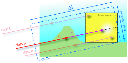
Figure 2: Sketch of the geometry relevant for neutrino simulations, see text for more details.

Second, a redefinition of the detection volume was done. The original ANIS version uses the concept of the detection volume [21]. This concept is useful for calculating event rates for a given neutrino flux $\Phi(E_{\nu},\theta_{\nu})$. The detection volume corresponds to the so called active volume in which potentially detectable neutrino interactions are simulated. In the original ANIS this volume is defined as a cylinder with z-axis parallel to the neutrino direction [15]. In our adapted version we kept the general idea of active volume but with some modifications, as shown in Fig. 2. As it can be seen from this figure, the active volume for a given incoming neutrino with energy $E_{\nu}$ is defined by a particular plane $A_{gen}$ and distance $\Delta L$. The plane $A_{gen}$ is the cross-sectional area of the detector volume and it was used as reference plane for the generation of incoming neutrinos. The area depends on the zenith angle $\theta$ of the incoming neutrino. The detector was modelled as a cylinder with radius $R$ and height $H$, The distance $\Delta L$ is the multiple, $n$, of the average lepton range $\left<R_{lep}(E_{lep})\right>$ [22]. Inside the active volume lepton tracks are also shown. Neutrinos with energy $E_{\nu}$ produce leptons with individual ranges, depending on the fraction of energy transfered. More precisely, the incoming neutrino is forced to interact in the active volume according to its interaction probability

$$P(E_{\nu},E_{lep},\theta)\simeq N_{A}\times\sigma(E_{\nu})\times\rho(Z)\times\Delta L,$$ (1)

where $\sigma(E_{\nu})$ is the total neutrino cross section, $\rho(Z)$ the local medium density and $N_{A}$ the Avogadro constant. $P(E_{\nu},E_{lep},\theta)$ is the probability that a neutrino with energy $E_{\nu}$ crossing the distance $\Delta L$ would produce a lepton with an energy $E_{lep}$. In this way the production vertex of the lepton is created. Then, the lepton propagates through the matter, losses some energy and decays (if it’s unstable) in the vicinity of the detector or inside the detector volume. In order to calculate physical quantities, one has to weight the events. A first weight is the interaction probability defined by Eq. (1). A second weight comes from the normalisation of the injected neutrino flux $\Phi(E_{\nu},\theta_{\nu})$

$$F^{w}_{\nu}=N_{gen}^{-1}\times\Delta T\times\int_{E_{min}}^{E_{max}}\Phi(E_{\nu})dE_{\nu}\times\int_{\theta_{min}}^{\theta_{max}}A_{gen}(\theta)\times d\Omega,$$ (2)

where $d\Omega=2\pi\sin\theta d\theta$ is the space angle, $\Delta T$ the observation time and $N_{gen}$ is the number of generated events from surface $A_{gen}$. Here, we assume the isotropic neutrino flux $\Phi(E_{\nu},\theta_{\nu})=\Phi(E_{\nu})$. The expected event rate of the neutrinos in the detector volume can be calculated from

$$N_{ratio}=F^{w}_{\nu}\times\sum_{i=1}^{N_{acc}}P_{i},$$ (3)

where $N_{acc}$ is the number of events triggering the detector and passing all quality cuts of the cascade analysis. The normalisation factor $F^{w}_{\nu}$ is chosen such that the rate of the neutrinos results in the total number of events per year.

Third, new tau lepton decay channels were implemented. In the original ANIS code the tau lepton decay is simulated using the code of TAUOLA [19]. The tau lepton decay is simulated by randomly choosing one event from a data base of pre-simulated events.

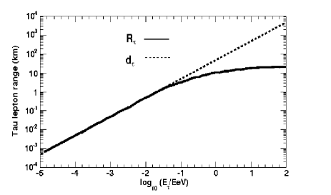
Figure 3: Tau lepton range $R_{\tau}$ and its decay length $d_{\tau}$ as a function of the energy.

Finally, the tau lepton decay routine was partly rewritten to take into account the processes of tauons escaping from the Earth’s surface and decaying in the atmosphere. In ANIS the tau is propagated in small energy steps until the age of the tau lepton exceeds the tau lepton lifetime. This procedure works quite well if the production and decay vertex are in the same medium (either in air or rock), but if the tau lepton crosses the Earth’s surfaces during its propagation inside the active volume, different amount of energy loss in the Earth’s crust and air have to be taken into account. In particular, when a tau lepton is generated in the Earth, it loses energy due to ionisation and radiation processes. These energy losses per unit length of crossed matter (in g/cm²) are usually approximated by a linear equation (continuous energy loss approach), which reads as

$$\frac{dE_{\tau}}{dX}=-\alpha-\beta(E_{\tau})\times E_{\tau},$$ (4)

where the factor $\alpha$ is due to the ionisation losses and $\beta$ is due to radiation losses. The factor $\alpha$ is negligible for ultra-high energies. The factor $\beta$ parameterises the tau lepton energy loss through bremsstrahlung, pair production, and photonuclear interaction.

Exemplary we have used two parameterisations: $\beta$ is linear dependent on energy

$$\beta_{A}(E_{\tau})\equiv 0.71\times 10^{-6}\mathrm{cm^{2}g^{-1}}+0.35\times 10^{-18}E\mbox{ }\mathrm{cm^{2}g^{-1}GeV^{-1}}$$ (5)

used by Aramo et al. in Ref. [8], and

$$\beta_{B}(E_{\tau})\equiv(1.508+6.3(E_{\tau}/10^{9})^{0.2})\times 10^{-7}\mathrm{cm^{2}g^{-1}}$$ (6)

from [15, 22, 23].

The lepton range, $R_{\tau}$, is given by the integral of the inverse of the tau lepton loss rate over the tau lepton energy

$$R_{\tau}=\frac{1}{\rho(z)}\int\frac{1}{dE/dX}dE.$$ (7)

Thus differences in $\beta$ will lead to different tau lepton ranges (length of the lepton track) and consequently influence the expected neutrino event rate and aperture calculations.

During a single step the distance passed by the tau lepton is evaluated according to the following formula

$$\Delta R_{\tau}=\frac{1}{\rho(z)\beta(E^{f}_{\tau})}ln(E_{\tau}^{f}/E_{\tau}^{i}),$$ (8)

where $E^{i}_{\tau}$ is the initial energy of the tau lepton and $E^{f}_{\tau}$ is the energy of the tau lepton after the distance $\Delta R_{\tau}$. During the energy step $\beta$ is constant. The distance $\Delta R_{\tau}$ is evaluated with the altitude dependent density $\rho(z)=\rho^{rock}(z)$ or $\rho(z)=\rho^{air}(z)$. $\rho^{rock}$ is the density of the Earth according to the Preliminary Earth Model [17] and $\rho^{air}$ is the air density calculated according to the US standard atmosphere (Linsley parameterisation) [24].

In Fig. 3 the tau lepton range in standard rock, $\rho=2.6\,\mathrm{g/cm^{3}}$ is shown for the parameter set $\beta_{B}$ based on calculations reported in [23]. One can see that the tau lepton range $R_{\tau}$ is of the order of about 10 km at 1 EeV. This value is about 5 times smaller than the tau lepton decay length, $d_{\tau}$, at the same energy. The decay length is given by $d_{\tau}=c\tau_{\tau}(E_{\tau}/m_{\tau})\sim 49\,\mathrm{km}\times(E_{\tau}/10^{18}\,\mathrm{eV})$ for tau lepton, where $c\tau_{\tau}=87.11$ is the tau lepton lifetime in $\mathrm{\mu m}$ and $m_{\tau}=1777.03\,\mathrm{MeV}$ is the tau lepton mass [25]. Thus, a tau lepton with an energy of about $1\,\mathrm{EeV}$ produced close to the Earth’s surface can escape from the Earth before decaying. One can note also, that the tau lepton decay length is about 490 km for a tau lepton energy of about 10 EeV. Therefore an emerging tau lepton can escape from the atmosphere, which is assumed to have an height of 100 km.

Applying the neutrino generation code, we obtain the tau lepton decay vertex position, the energy and momentum of the decay products for simulated neutrino showers with a given energy. AIRES was used to generate the longitudinal profiles of charged particles and the energy deposit based on the ANIS output. A special mode was used to inject simultaneously several particles at a given interaction point. The emission of fluorescence light by the shower together with its propagation towards the detector and the response of detector itself, including electronics and trigger, were simulated by the Offline software. Finally on the basis of the algorithms implemented in the Offline software the first two trigger levels called First Level Trigger (FLT) and Second Level Trigger (SLT) were simulated [6]. After the simulated events had passed the FLT threshold trigger (at least one pixel), a search for pattern consisting of 5 pixels was performed according to the SLT algorithm. In this way the trigger efficiency of the FD for a given neutrino energy can be defined as

$$\Sigma(E_{\nu})=\frac{N_{SLT}}{N_{Aires}}\times\gamma$$ (9)

where $N_{Aires}$ is the the number of AIRES tau showers simulated for a given neutrino energy, $N_{SLT}$ the number of showers passing the SLT condition and $\gamma$ the duty cycle of fluorescence detector.

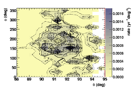
Figure 4: Event rate as a function of azimuth and zenith for the detector volume in the case of quasi-horizontal $\nu_{\tau}$ showers, assuming $E_{\tau}^{th}=1\,\mathrm{EeV}$, a WB flux, $\Delta L=15\left<R_{\tau}(E_{\tau})\right>$, $\beta_{B}$, 10% duty cycle of FD detector.

III Results

Simulations are done for neutrino showers ranging from 1-100 EeV. Usually 500.000 events are generated on the surface $A_{gen}$ for different azimuth and zenith angles. A cuboid with an area of $50\times 60\,\mathrm{km^{2}}$ and height of 10 km positioned at 1430 m a.s.l. was used as detector volume ($\equiv V_{FD}$). It agrees quite well with the detection volume seen by FD.

In Fig. 4 the map of the expected event rate in $\mathrm{yr^{-1}}$ as a function of the incoming direction $(\theta,\phi)$ is shown. Significant directional differences in the number of expected events are seen. The largest rate is for almost horizontal neutrinos with the zenith $\theta$ in the range between 89^∘-93^∘ and azimuth $\phi$ in the range between 100^∘ and 270^∘ (North-West-South). However, some peaks in the rate distribution exist for azimuth of about 350^∘ (East). This behaviour is due to the fact that the Auger site is surrounded by the Andes on the West and smaller but closer mountains in the East (see the map shown in Fig. 1).

TABLE I: Expected event rate in yr^-1 for quasi-horizontal showers. The rate has been evalueated for different incoming $\nu_{\tau}$ directions and at $E^{th}_{\tau}=1\,\mathrm{EeV}$ assuming the FD detection volume $V_{FD}$. The WB neutrino flux, $\beta_{B}$ and 10% duty cycle of FD detector have been assumed.

	Azimuth		$N^{FD}_{DW}$		$N^{FD}_{QH}$
	(deg)		(yr-1)		(yr-1)
Theta			85∘-90∘		85∘-95∘
East	-45-45		0.0005		0.009
North	45-135		0.0007		0.012
West	135-225		0.0027		0.023
South	225-315		0.0007		0.009
Total			0.0046		0.052

On the other words the correlations between the calculated distribution of the event rate and the topography of the Auger site is well seen (mountain effect). The mountain effect is much more pronounced for $\nu_{\tau}$ showers very close to the horizon and less obvious for larger zenith angle ranges. A quantitative analysis of this effect for horizontal showers is presented in Tab. I and for up-going showers in Tab. II.

In Tab. I, the dependence of the expected number of events from the direction of incoming neutrinos is well seen. For example, in the case of quasi-horizontal (QH) showers the expected ratio from the West is about 3 times larger than the ratio from the East (for downward-going shower (DW) the ratio from the West is about 5 times larger than from the East). Note also that the rate in the case of QH showers is about one order larger than the rate for downward-going showers.

TABLE II: Expected event rate in yr^-1 for up-going neutrino showers for different ranges of zenith angle for $E_{th}=1\,\mathrm{EeV}$, $\beta_{B}$, FD detector volume $V_{FD}$, WB flux and 10% duty cycle of FD detector. $N^{FD}_{SP}$ is the rate calculated according to the spherical model of the Earth with the detector positioned at 10 m above the surface.

	class A+B+C		class A		Sphere
$\Theta$	$N^{FD}$	$N_{acc}$	$N^{FD}$	$N_{acc}$	$N^{FD}_{SP}$	$\frac{B}{A+B+C}$
(deg)	(yr-1)		(yr-1)		(yr-1)	(%)
90-92	0.0219$\pm$1%	34205	0.0108	1209	0.0105	48
92-94	0.0168$\pm$2%	9895	0.0133	1248	0.0140	24
94-96	0.0068$\pm$15%	199	0.0060	165	0.0059	11
96-98	0.0008$\pm$43%	29	0.0008	27	0.0010	6

In Tab. II the expected event rates for different ranges of zenith angle are listed. The rate is dominated by events close to the horizon and gets only small contributions at larger zenith angles. This is due to the fact that in the case of up-going $\nu_{\tau}$ the regeneration effect plays a important role. A high-energy $\nu_{\tau}$ interacts in the Earth producing a tau lepton which in turn decay into a $\nu_{\tau}$ with lower energy due to its short lifetime. The regeneration chain $\nu_{\tau}\rightarrow\tau\rightarrow\nu_{\tau}\rightarrow$ … continues until the tau lepton reaches the detector (in our case the active volume). This effect leads to a significant enhancement of the tau lepton flux up to about 40% more than the initial cosmic flux of tau neutrinos of energies between $10^{6}-10^{8}$ GeV [26, 27].

Additionally, the rate for the different classes of events defined in Fig. 2 is presented. Class A has the production vertex in the Earth (below horizon) and decay vertices inside $V_{FD}$. The class B and C have production vertices above the horizon and decay vertices inside $V_{FD}$ (the contribution of class C is about one order smaller than class B). In principle the difference between these classes are a measure of the influence of the mountain effect reflected in a zenith dependent event rate [28]. As it can be seen from this Table (the last column), the contribution of mountains to the total $\nu_{\tau}$ event rate is significant. For example, for nearly horizontal $\nu_{\tau}$ showers within zenith angle less than 2 degrees below the horizon, the contribution is about 50% while for larger zenith angle ranges it is on average less than 24%. We come to the same conclusion if we estimate the mountain effect taking into account the calculation with the simple spherical model of the Earth because the rate calculated in this case agrees very well with the rate calculated for class A.

In Fig. 5A the estimation of the aperture for up-going $\nu_{\tau}$ showers is shown. We define the aperture by

$$A(E_{\nu})=N_{gen}^{-1}\times\sum_{i=1}^{N_{\tau}}\sum_{j=1}^{N_{\theta,\phi}^{acc}}P_{i,j}(E_{\nu},E_{\tau},\theta)\times A_{j}(\theta)\times\Delta\Omega,$$ (10)

where $N_{\tau}$ is the number of tau leptons with energy $E_{\tau}$. $E_{\nu}$ is the initial neutrino energy, $N_{\theta,\phi}^{acc}$ is the number of tau leptons coming from a given direction inside $V_{FD}$ and passing our cuts. The aperture was calculated according to the parameterisation of $\beta_{A}$ and $\beta_{B}$. Different parameterisations lead only to small differences in the calculated aperture. Additionally, in Fig. 5A the aperture calculated by [11] is shown. One can see a fairly good agreement within 20% between the results presented in this paper and aperture calculated by [11] for energies between 1 EeV and 10 EeV. For larger energies, above 100 EeV, our aperture decreases with increasing of neutrino energies. This is due to the fact that for these energies the tau lepton decay length in air is extremely large (above 5000 km), then the emerging tau lepton from the Earth will escape from the detector, or even from the atmosphere.

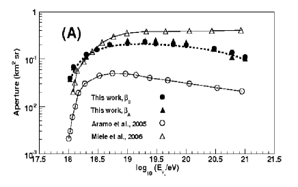
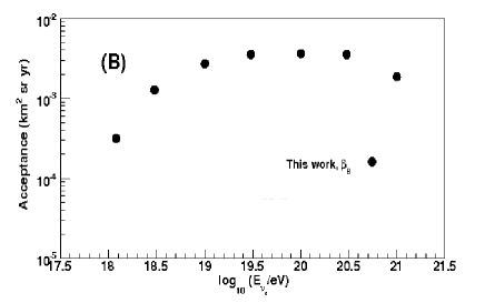
Figure 5: (A) The effective aperture for the Pierre Auger Observatory, $A(E_{\nu_{\tau}})$, for $E_{\tau}>10^{18}$ eV, $90^{\circ}<\theta<95^{\circ}$ ,$0^{\circ}<\phi<360^{\circ}$, $V_{FD}$ and $N_{gen}=200000$; (B) The effective acceptance $A_{c}(E_{\nu})$ for the Pierre Auger Observatory. The 10% duty cycle of FD was included.

In Fig. 5B the FD acceptance for Pierre Auger Observatory is shown. The acceptance is calculated from

$$A_{cc}(E_{\nu})=A(E_{\nu})\times\Sigma(E_{\nu})|_{E_{\tau}>1\,\mathrm{EeV}}.$$ (11)

assuming that a trrigered event is seen at least by one fluorescence eye of Pierre Auger Observatory. The acceptance increases from $0.001\,\mathrm{km^{2}\,sr\,yr}$ to about $0.003\,\mathrm{km^{2}\,sr\,yr}$ between 30 EeV and 1000 EeV. The acceptance does not saturate but drops at larger energies since tau leptons at such energies escape unseen from the detector volume $V_{FD}$ lowering the acceptance. The calculated acceptance differs about two orders of magnitude from the calculated aperture.

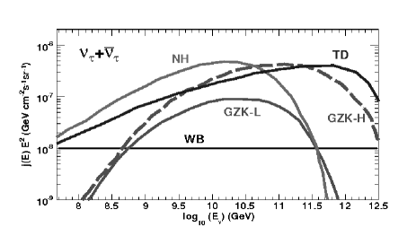
Figure 6: Tau neutrino and anti-neutrino fluxes from various models, taken from Ref. [8].

Finally, in Tab. III the rate for different injected neutrino fluxes shown in Fig. 6, based on our acceptance and apperture calculation, are listed. The WB rate is obtained for Waxman-Bahcall bound. In this paper we use the conservative estimate of this bound $\Phi(E_{\nu_{\tau}+\bar{\nu}_{\tau}})=1\times 10^{-8}E^{-2}\mbox{ (GeV s${}^{-1}$ cm${}^{-2}$ sr)}$. Other rates are reported for the same neutrino fluxes considered in section 2 of Ref. [8]. The two GZK fluxes refer to the two possible scenarious for cosmogenic neutrinos, which are those produced from an initial flux of UHE protons. Instead the NH (New Hadrons) and TD (Topological Defects) cases are two examples of exotic models. As one can see from Tab. III, the number of expected events equals about 1 neutrino event per 2 years in the case of our aperture calculation. Taking into account the FD detector properties rate is about one order smaller, but neutrino event still can be observable by Auger detector during a few decade of operational.

TABLE III: Expected event rate in yr^-1 for the different neutrino fluxes based on our aperture ($N_{Aper}$) and acceptance calcultion ($N_{Acc}$). Results for $\nu_{\tau}$ events with zenith angle in the range $90^{\circ}-95^{\circ}$, assuming $E_{\tau}^{th}=1\,\mathrm{EeV}$, a WB flux, $\Delta L=15\left<R_{\tau}(E_{\tau})\right>$, $\beta_{B}$, 10% duty cycle of FD detector.

			WB		GZK-L	GZK-H		TD	NH
	$N_{Aper}$		0.044		0.456	0.699		0.546	1.478
	$N_{Acc}$		0.004		0.042	0.072		0.053	0.137

Note that event rate becomes larger for lower threshold energy. In fact FD detector can record also the shower with enegies above $10^{17}$ eV.

IV Summary

A tool to simulate neutrino propagation and interaction in the Earth and in the atmosphere taking into account the local topographic conditions, was presented. A detailed investigation of neutrino induced showers was performed. The focus was put on the neutrino sensitivity for the FD detector of the Pierre Auger Observatory and therefore we have used the digital elevation map for this site. The probability map (event rate distribution) and the aperture were calculated and the impact of the mountains surrounding the Auger site was quantified. General features are consistent with previous results, but as a consequence of the surrounding mountains a pronounced variation of the event rate as a function of the azimuth is seen.

References

- [1] J. N. Bahcall and E. Waxman, “High energy astrophysical neutrinos: The upper bound is robust,” Phys. Rev., vol. D64, p. 023002, 2001.
- [2] A. V. Olinto, “Ultra High Energy Cosmic Rays: The theoretical challenge,” Phys. Rept., vol. 333, pp. 329–348, 2000.
- [3] P. Bhattacharjee and G. Sigl, “Origin and Propagation of Extremely High Energy Cosmic Rays,” Phys. Rept., vol. 327, pp. 109–247, 2000.
- [4] V. Berezinsky and G. T. Zatsepin, “Cosmic rays at ultra high energies (neutrino?),” Phys. Lett. B, vol. 28, p. 423, 1969.
- [5] S. Fukuda et al., “Constraints on Neutrino Oscillations Using 1258 Days of Super-Kamiokande Solar Neutrino Data,” Phys. Rev. Lett., vol. 86, p. 5656, 2001.
- [6] J. Abraham et al., “Properties and performance of the prototype instrument for the Pierre Auger Observatory,” Nucl. Instrum. Meth., vol. A523, pp. 50–95, 2004.
- [7] X. Bertou, P. Billoir, O. Deligny, C. Lachaud, and A. Letessier-Selvon, “Tau neutrinos in the Auger Observatory: a new window to UHECR sources,” Astropart. Phys., vol. 17, pp. 183–193, 2002.
- [8] C. Aramo et al., “Earth-skimming UHE Tau Neutrinos at the Fluorescence Detector of Pierre Auger Observatory,” Astropart. Phys., vol. 23, pp. 65–77, 2005.
- [9] E. Zas, “Neutrino detection with inclined air showers,” New J. Phys., vol. 7, p. 130, 2005.
- [10] L. Anchordoqui, T. Han, D. Hooper, and S. Sarkar, “Exotic Neutrino Interactions at the Pierre Auger Observatory,” Astropart. Phys., vol. 25, pp. 14–32, 2006.
- [11] G. Miele, S. Pastor, and O. Pisanti, “The aperture for UHE tau neutrinos of the Auger fluorescence detector using a Digital Elevation Map,” Phys. Lett. B, vol. 634, pp. 137–142, 2006.
- [12] Department of the Navy, “OC 2902 Web Based Course Reference Material.” [Online]. Available: http://www.oc.nps.navy.mil/oc2902w/sitemap.htm
- [13] S. Sciutto, “AIRES a system for air shower simulation, version 2.6.0 (2002).” [Online]. Available: http://www.fisica.unlp.edu.ar/auger/aires/
- [14] Pierre Auger Collaboration, T. Paul et al., “The Offline software framework of the Pierre Auger Observatory,” Proc. 29th Intern. Cosmic. Ray Conf., Pune, 8, 343, 2005.
- [15] A. Gazizov and M. P. Kowalski, “ANIS: High Energy Neutrino Generator for Neutrino Telescopes,” Comput. Phys. Commun., vol. 172, pp. 203–213, 2005.
- [16] AMANDA Collaboration, “Antarctic Muon and Neutrino Detector Array at the South Pole (AMANDA), E. Andres et al., astro-ph/0009242.” [Online]. Available: http://amanda.wisc.edu/
- [17] A. M. Dziewonski and D. L. Anderson, “Preliminary reference earth model,” Phys. Earth Planet. Interiors, vol. 25, pp. 297–356, 1981.
- [18] H. Lai and et al., “Global QCD Analysis of Parton Structure of the Nucleon CTEQ5 Parton Distributions,” hep-ph/9903282, 1999.
- [19] S. Jadach, Z. Was, R. Decker, and J. H. Kuhn, “The tau decay library TAUOLA: Version 2.4,” Comput. Phys. Commun., vol. 76, pp. 361–380, 1993.
- [20] Consortium for Spatial Information (CGIAR-CSI). [Online]. Available: http://srtm.csi.cgiar.org/
- [21] M. Kowalski, “On the reconstruction of cascade-like events in the AMANDA detector,” Diploma Thesis, Humboldt University, Berlin, 2000.
- [22] S. I. Dutta, M. H. Reno, I. Sarcevic, and D. Seckel, “Propagation of muons and taus at high energies,” Phys. Rev., vol. D63, p. 094020, 2001.
- [23] J.-J. Tseng et al., “The energy spectrum of tau leptons induced by the high energy Earth-skimming neutrinos,” Phys. Rev., vol. D68, p. 063003, 2003.
- [24] United States Committee on Extension and to the Standard Atmosphere (COESA), “US Standard Atmosphere Model.” [Online]. Available: http://nssdc.gsfc.nasa.gov/space/model/atmos/us\_standard.html
- [25] D. E. Groom et al., “Review of particle physics,” The European Physical Journal, vol. C15, pp. 1+, 2000. [Online]. Available: http://pdg.lbl.gov
- [26] J. Jones, I. Mocioiu, M. H. Reno, and I. Sarcevic, “Tracing very high energy neutrinos from cosmological distances in ice,” Phys. Rev., vol. D69, p. 033004, 2004.
- [27] E. Reya and J. Rodiger, “Signatures of cosmic tau-neutrinos,” Phys. Rev., vol. D72, p. 053004, 2005.
- [28] L. Anchordoqui, A. Cooper-Sarkar, D. Hooper, and S. Sarkar, “Probing low-x QCD with ultra-high energy cosmic neutrinos at Auger,” hep-ph/0605086, 2006.