Cosmic microwave background limits on spatially homogeneous cosmological models with a cosmological constant.

Abstract

We investigate the effect of dark energy on the limits on the shear anisotropy in spatially homogeneous Bianchi cosmological models obtained from measurements of the temperature anisotropies in the cosmic microwave background. We shall primarily assume that the dark energy is modelled by a cosmological constant. In general, we find that there are tighter bounds on the shear than in models with no cosmological constant, although the limits are (Bianchi) model dependent. In addition, there are special spatially homogeneous cosmological models whose rate of expansion is highly anisotropic, but whose cosmic microwave background temperature is measured to be exactly isotropic at one instant of time.

Department of Mathematics and Statistics, Dalhousie University, Halifax, Nova Scotia, Canada, B3H 3J5

1 Introduction

Observations suggest that the Universe has $0.98\leq\Omega_{tot}\leq 1.08$ with radiation (R), baryons (B), dark matter (DM) and dark energy (DE) each contributing $\Omega_{R}\simeq 5\times 10^{-5},\Omega_{B}\simeq 0.04,\Omega_{DM}\simeq 0.26,\Omega_{DE}\simeq 0.7,$ respectively [1], where the variables $\Omega_{i}=\rho_{i}/\rho_{c}$ give the fractional contribution of different components of the Universe ($i$ denoting baryons, dark matter, radiation, etc.) to the critical energy density $\rho_{c}=3H^{2}_{0}/8\pi G$, where $H_{0}=(\dot{a}/a)_{0}$ is the present Hubble expansion rate. Consequently, we have that $\Omega_{0}\equiv\Omega_{R}+\Omega_{B}+\Omega_{DM}\sim 0.3$. The simplest model for a fluid with negative pressure is the cosmological constant [2] whence nearly seventy per cent of the energy density in the Universe is unclustered and exerts negative pressure; $\Omega_{\Lambda_{0}}\equiv\Omega_{DE}\sim 0.7$.

It is of interest to study the effect of dark energy on the cosmological limits from cosmic microwave background (CMB) measurements on the shear (and the rotation, etc.), especially in spatially homogeneous (SH) cosmological models. In the presence of the cosmological constant, an SH universe that is very nearly flat now and that was very nearly flat at the time of last scattering can become significantly negatively curved at intermediate periods. At earlier times the matter dominates and the curvature is dynamically negligible, while at later times $\Omega_{\Lambda}$ can dominate. For a currently almost flat universe with parameters close to the observed values of $\Omega_{\Lambda_{0}}\sim 0.7$ and $\Omega_{0}\sim 0.3$, the curvature is at most only a few percent. At intermediate times, however, the curvature can be dynamically significant.

The observed temperature anisotropy (from COBE and WMAP [3]) of the CMB radiation, $\Delta T/T$, on large angular scales is determined by the value of the shear at the surface of last scattering of the radiation. To evaluate large-scale anisotropies we must evaluate the peculiar redshift a photon will feel from the epoch of last scattering (${\it ls}$) until now $(0)$ by integration along null geodesics in the background spacetime.

The usual paradigm invoked to understand cosmological observations, motivated by inflation and consistent with the smoothness of the CMB, is that the Universe was spatially homogeneous and isotropic spacetime at early times. The theory is then that some physical mechanism (such as inflation) generated perturbations that subsequently evolved through gravitational collapse to form the structures we now observe. Within this paradigm, the Universe is closely modelled by a Friedmann-Robertson-Walker (FRW) cosmology at all times since the earliest epoch (and particularly since recombination). In such models it is often the case that the integrated effect from a small shear is not important.

We utilize dynamical systems methods using expansion-normalized variables in SH cosmological models [4], generalized to include a cosmological constant, to revisit the cosmological constraints on the Hubble-normalized shear scalar $\Sigma=\sigma/(\sqrt{3}H)$ (for example) from CMB anisotropy measurements.

2 Background

Bianchi models provide a description of general SH anisotropic cosmologies. There are distinct features depending on the overall geometry and homogeneity class of the model [5]. In a pioneering paper, Collins and Hawking used analytical arguments to find upper bounds on the amount of shear (and vorticity) in the Universe today, from the absence of any detected CMB anisotropy [6]. A detailed numerical analysis of such models [7] used experimental limits on the dipole and quadrupole to refine limits on the universal shear (and rotation). More recently, it has been argued [8] that there is no ‘isotropy problem’ in Bianchi type VII_h cosmological models in which shear (and vorticity) have decayed only logarithmically since the Planck time, in that the present amplitude of CMB fluctuations is compatible with current observational limits in these models.

The limits could be strengthened in a number of ways; for example, if we assume particular classes of cosmological models (i.e., spatially homogeneous models) for which exact evolution laws are known we can replace assumptions and approximations by exact relations. For particular Bianchi models with specific evolution equations, stronger limits are indeed possible. In particular, in general shear anisotropy grows with time (i.e., Bianchi models do not generically isotropize). However, for very special models (i.e., not generic) of Bianchi type I and V the anisotropy decays, and hence much stronger limits on present day shear may be obtained in these models.

In particular, in [9] it was shown that small quadrupole anisotropies in the CMB imply severe limits on spacetime anisotropy in a Bianchi type I model (assumed to be a small perturbation of a FRW model). Using an exact Bianchi I cosmological solution, the quadrupole component of CMB temperature distribution found by COBE [3] (expressed as an upper limit on $\Delta T/T$), implies that $\Sigma_{0}\leq 2\times 10{{}^{-9}}$. Similarly, strong limits can be obtained in Bianchi type V models (and a special class of spatially homogeneous Bianchi type VII_h models [8]). However, such severe limits are not generic.

The above limits on the shear (and rotation) are not based on ‘full sky’ maps; only the simple quadrupole (and not higher multipoles, which produce hotspots/spirals) is utilized. In general SH models the distorted quadrupole is combined with spiral geodesic motion, and by solving the geodesic equations describing the motion of photons numerically, limits can be derived from the whole COBE sky map. We note that unlike the open type VII_h models (for example), the closed Bianchi type IX models exhibit neither geodesic focusing nor the spiral pattern, even in the presence of vorticity [7].

A special class of Bianchi type VII_h models, which have a logarithmic dynamical evolution and $\Sigma$ that is effectively ‘frozen in’ at late times, were studied in [7] and it was concluded that limits on the shear are as strong as $|\Sigma_{0}|\sim 10^{-9}$ in the real Universe. In further work [10], the large-scale cosmic microwave background anisotropies in spatially homogeneous, globally anisotropic cosmologies were investigated, and improvements on previous bounds on the total shear in the Universe were obtained by performing a statistical analysis to constrain the allowed parameters of a Bianchi model of type VII_h using the cumulative data from COBE. Consequently, very strong upper limits on the amount of shear (and vorticity) were obtained; limits which are typically one to two orders of magnitude higher than constraints relying entirely on the quadrupole. Moreover, in discarding information from higher moments, the comparison is not sensitive to the small-scale structure present in anisotropic models that is associated either with the spiral pattern or with geometrical focusing when $\Omega<1$. This bound ([10]) can be improved upon by a factor of $\sqrt{3}$ by using different statistics [11].

If the CMB fluctuations about isotropy are small, then so are deviations from spatial homogeneity and isotropy [12], provided that the Universe after last scattering can be modelled as exactly dust (plus collision-free radiation, and may include a cosmological constant). Model-independent limits on the present day strengths of large-scale shear in the Universe in the important case of an almost isotropic CMB, which also take into account inhomogeneities as well (assuming constraints on the size of temporal and spatial derivatives), can then be obtained. A general limit on the present value of $\Sigma$ can be obtained using the quadrupole and octopole; $\Sigma_{0}\leq 10{{}^{-4}}$ [12]. This general limit is a much weaker limit on the shear than discussed above, which implies that the Bianchi VII_h models (for example) are too special to draw conclusions from because of their atypical evolution. However, it was shown [12] that stronger limits on the shear [7] can be recovered in a (Bianchi VII_h) model which is Bianchi I to first order [12].

It is worth mentioning that since the Einstein equations are highly non-linear, the limit as the (anisotropic) curvatures tend to zero (in some appropriate sense) in Bianchi models does not necessarily produce the same results as those in a Bianchi I model with zero curvature. Although limits can often be strengthened by considering a particular class of Bianchi cosmological models for which exact evolution equations are known, the results are not generic. Indeed, for very specific models of Bianchi type I and V which isotropize, very severe limits are obtained. In general, specific limits are obtained in each class of SH models, which include integrated and non-integrated effects, which combine distorted quadrupole and spiral geodesic motion, and which include limits from numerical and statistical analyses derived from the full COBE sky map.

3 Analysis

We shall investigate anisotropic cosmological models with pressureless matter (dust) and a cosmological constant (assumptions which are justified since recombination). Typically, if the shear $\Sigma$ is small throughout the evolution since recombination, the integrated effect on the CMB is not important. However, if the shear is not small the effect can be important.

In the case of a Bianchi type I model, and exact solution (for dust and a cosmological constant) is again possible. We find that

$$\Sigma^{2}=\frac{\Sigma_{0}{{}^{2}}e^{-3t}}{\Sigma_{0}{{}^{2}}e^{-3t}+\Omega_{\Lambda_{0}}e^{3t}+\Omega_{0}}\approx\frac{\Sigma_{0}{{}^{2}}e^{-3t}}{\Omega_{\Lambda_{0}}e^{3t}+\Omega_{0}},$$ (1)

where $\Sigma_{0}$ (for example) is the value of the shear at the present logarithmic time $t=0$, and the constants satisfy

$$\Omega_{0}+\Omega_{\Lambda_{0}}+\Sigma_{0}^{2}=1.$$ (2)

The approximation can be integrated exactly to give

$$\int^{0}_{t_{ls}}\Sigma dt\approx\frac{2\Sigma_{0}}{3\Omega_{0}}\left[e^{-\frac{3}{2}t_{ls}}(\Omega_{\Lambda_{0}}e^{3t_{ls}}+\Omega_{0})^{\frac{1}{2}}-1\right]\approx\frac{2}{3}e^{-\frac{3}{2}t_{ls}}\frac{\Sigma_{0}}{\sqrt{\Omega_{0}}},$$ (3)

where we will use $t_{ls}=-7$ as the logarithmic time of last scattering. Imposing the quadrupole limit

$$\int^{0}_{t_{ls}}\Sigma dt<10^{-5},$$ (4)

we then obtain

$$\Sigma_{0}<4.13\times 10{{}^{-10}}\sqrt{\Omega_{0}}.$$ (5)

Therefore, the limit is strengthened (for a smaller value of $\Omega_{0}$, corresponding to a larger $\Omega_{\Lambda_{0}}$) over the case with no cosmological constant (for example, by a factor of about 2 if $\Omega_{0}=0.3$). The physical reason for this strengthening is that for a more dominant cosmological constant (as measured by $\Omega_{\Lambda_{0}}$), the Hubble-normalized shear $\Sigma$ tends to zero faster (see equation (1)). As a result, given a fixed amount of integrated shear (e.g., $10^{-5}$), the present day value $\Sigma_{0}$ is smaller in the presence of a dominant $\Omega_{\Lambda_{0}}$.

The limit on the shear in Bianchi I models from the quadrupole is strengthened when a non-zero cosmological constant is present. There will be similar results for Bianchi type V models, which also isotropize to the future (and, in addition, for Bianchi type VII_h models). However, for general models which do not isotropize to the future (without the presence of dark energy), the limits on the shear will become much much tighter.

As an illustration, let us consider the locally-rotationally symmetric (LRS) Bianchi type III cosmological models. The evolution equations for expansion-normalized variables can be obtained by setting $k=1/2$ in [13, Section 2.1.2] and including a cosmological constant:

$$\Sigma_{\times}^{\prime} =(q-2)\Sigma_{\times}-\Omega_{k}$$ (6)

$$\Omega_{k}^{\prime} =2(q+\Sigma_{\times})\Omega_{k}$$ (7)

$$\Omega_{\Lambda}^{\prime} =2(q+1)\Omega_{\Lambda},$$ (8)

where

$$q =2\Sigma_{\times}^{2}+\tfrac{1}{2}\Omega-\Omega_{\Lambda}$$ (9)

$$\Omega =1-\Sigma_{\times}^{2}-\Omega_{k}-\Omega_{\Lambda}.$$ (10)

Here, $\Sigma_{\times}$ is the shear, $\Omega_{k}$ is the spatial curvature, $\Omega_{\Lambda}$ is the density parameter for the cosmological constant, $\Omega$ is the density parameter for dust, and $q$ is the deceleration parameter.

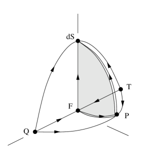
Figure 1: State space of LRS Bianchi type III cosmological models with dust and a cosmological constant. Arrows indicate the direction of evolution. The shaded surface indicates a set of initial conditions at present time yielding exactly isotropic CMB.

Shown in Figure 1 is the state space of LRS Bianchi type III cosmological models with dust and a cosmological constant. The state space shown is a quarter of a unit sphere, with equilibrium points representing the flat FRW solution (F), the de Sitter solution (dS), the two Kasner solutions (T and Q) and the plane wave solution (P) (located at $\Sigma_{\times}=-\frac{1}{2}$). The FRW solution with a cosmological constant is represented by the vertical line F-dS. The state space is divided into regions A and B (separated by the surface F-P-dS), according to whether the shear $\Sigma_{\times}$ changes sign over the course of evolution.

The observed CMB temperature $T$ is given in terms of an integral of the quantity $s$, which in this case only depends on $\Sigma_{\times}$ and one direction cosine $K_{2}$:

$$T=T_{ls}\exp\left[-\int_{t_{ls}}^{0}(1+s)\ dt\right],$$ (11)

$$s=-(1-3K_{2}^{2})\Sigma_{\times},$$ (12)

$$K_{2}^{\prime}=-3(1-K_{2}^{2})K_{2}\Sigma_{\times}.$$ (13)

Following the calculation in [14], the observed CMB temperature $T$ is then given by

$$T=T_{ls}e^{-t_{ls}}\frac{e^{2\beta_{0}}}{\sqrt{e^{6\beta_{0}}+(1-e^{6\beta_{0}})K_{2}^{2}(0)}},$$ (14)

where $\beta_{0}$ is the integrated shear:

$$\beta_{0}=-\int_{t_{ls}}^{0}\Sigma_{\times}\ dt.$$ (15)

If $\beta_{0}=0$, then the CMB temperature is exactly isotropic.

If the shear variable $\Sigma_{\times}$ does not change sign (e.g., for initial conditions in the region B), then the viable models stay close to FRW during the whole evolution. Numerically integrating the null geodesic equations shows that, as expected, the limits on the shear are much tighter in the presence of a cosmological constant, tending to the Bianchi I constraints in the limit of negligible curvature.

It is known that there are spatially homogeneous cosmological models whose CMB temperature is measured to be exactly isotropic (by all fundamental observers), and hence indistinguishable from FRW, at one instant of time, but whose rate of expansion is highly anisotropic [14] (recall that we only observe the CMB at one instant of time). These results do not contradict bounds on the shear found by [6, 7, 8], who restrict attention ab initio on spatially homogeneous models close to FRW. In particular, in the Bianchi type III models under investigation but with dust only (and no cosmological constant), if $\Sigma_{\times}$ can change sign (i.e., for initial conditions in the region A [very close to the orbit F-P]), then the models need not stay close to FRW during the whole evolution and it is possible for the CMB to be exactly isotropic at one instant of time. From Figure 1, the curve at the base of the shaded surface shows that $\Sigma_{0}$ can be very large (close to one half), while giving an exactly isotropic CMB. Initial conditions in a small neighbourhood of this curve gives a close-to-isotropic CMB.

Similarly, in Bianchi type III models with dust and a positive cosmological constant, there is a surface of initial conditions yielding an exactly isotropic CMB and a small neighbourhood of this surface gives a close-to-isotropic CMB. The value of $\Sigma_{0}$ on this surface is smaller than the value of $\Sigma_{0}$ on the curve (i.e., adding a cosmological constant tightens the bound on $\Sigma_{0}$). Note that the sign change in $\Sigma_{\times}$ occurs (during the evolution) for all initial conditions on the indicated surface. As a result, imposing a limit on the CMB quadrupole will yield a looser bound on $\Sigma_{0}$ than in Bianchi I models (or any model in which the shear components cannot change sign; a sign change can lead to a cancellation in the integral $\int\Sigma dt$).

The same argument applies to non-LRS models, and generally in Bianchi models of all types, where there are sign changes in the shear [14]. However, complications in the analysis can arise because there may be no exactly isotropic surface to base the calculation on. In addition, obtaining constraints based upon the octopole may also pose problems, since $\int\Sigma dt$ may be a poor approximation for the octopole.

4 Discussion

The WMAP data provide some of the most accurate measurements yet of the CMB and contribute to high accuracy determinations of cosmological parameters [3]. However, there are several studies that show that at large scales, the CMB is not statistically isotropic and Gaussian [15]. In [16], a possible detection of a correlation between several independently discovered anomalies in the CMB sky measured by the WMAP data and a Bianchi Type VII_h template [7] was reported. The predictions for the CMB anisotropy patterns arising in Bianchi type VII_h universes which include a dark energy component were presented in [17], and it was found that including a term $\Omega_{\Lambda}>0$, can lead to the same observed structure as in the best-fit Bianchi type VII_h model of [16]. Although the best-fit Bianchi type VII_h model is not compatible with measured cosmological parameters, it was shown that removing a Bianchi component from the WMAP initial data release can account for several large angular scale anomalies and yield a corrected sky that is statistically isotropic. It was concluded that in the absence of an unknown systematic effect which could explain both the anomalies and the correlation, the WMAP data require an addition to the standard cosmological model that resembles the Bianchi morphology [16].

We have only discussed orthogonal spatially homogeneous models here. Expanding SH perfect fluid cosmological models with a constant equation of state parameter $\gamma$ with a non-geodesic ‘tilting’ fluid congruence were studied in [18]. It was shown that for stiff equations of state the tilt can give rise to an effective quintessential, or even phantom-like, equation of state. More importantly, it is of interest to investigate the effect of tilt on CMB radiation observations from the perspective of the observers moving with the fluid matter congruence and, in particular, to determine whether the tilt can significantly affect the constraints on the shear in SH models.

4.1 acknowledgements

We would like to acknowledge funding, in part, from NSERC of Canada. We thank Sigbjorn Hervik for discussions.

References

- [1] D. N. Spergel et al., Astrophys. J. Suppl., 148 175 (2003); M. Tegmark, et al., Phys. Rev. D, 69 103501 (2004); A. G. Reiss et al., Astrophys. J., 607 665 (2004).
- [2] T. Padmanabhan, Phys. Rept. 380 235 (2003) [hep-th/0212290]; Current Science, 88 1057 (2005) [astro-ph/0411044]; gr-qc/0503107.
- [3] C.L. Bennett et al., Ap. J. Suppl., 148 1 (2003).
- [4] J. Wainwright and G. F. R. Ellis (editors), Dynamical Systems in Cosmology, Cambridge University Press (1997).
- [5] G. F. R. Ellis and M. A. H. MacCallum, Commun. Math. Phys. 12 108 (1969).
- [6] C.B. Collins and S.W. Hawking, Mon. Not. R. Astron. Soc., 162, 307 (1973); A.G. Doroshkevich et al., Sov. Astr. 18, 554 (1975); C.B. Collins and S.W. Hawking, Astrophys. J. 180 317 (1973).
- [7] J. D. Barrow, R. Juszkiewicz and D. H. Sonoda, Mon. Not. R. Astron. Soc. 213 917 (1985).
- [8] J. D. Barrow, Phys. Rev. D 51 3113 (1995)
- [9] E. Martinez-Gonzalez and J.L. Sanz, Astron. & Astrophys. 300 346 (1995).
- [10] E. F. Bunn, P. G. Ferreira and J. Silk, Phys. Rev. Lett. 77 2883 (1996).
- [11] A. Kogut, G. Hinshaw and A. Banday, Phys. Rev. D [preprint astro-ph/9601060] (1996).
- [12] W. R. Stoeger, R. Maartens, and G. F. R. Ellis, Astrophys. J. 443, 1 (1995); R. Maartens, G. F. R. Ellis, and W. R. Stoeger, Phys. Rev. D 51, 1525 & 5942 (1995) & Astron. & Astrophys. 309, L7 (1996).
- [13] U. S. Nilsson, C. Uggla and J. Wainwright, Gen. Rel. Grav. 32, 1319 (2000).
- [14] W. C. Lim, U. S. Nilsson and J. Wainwright, Class. Quantum Grav. 18 5583 (2001).
- [15] A. de Oliveira-Costa et al., Phys. Rev. D, 69, 063516 (2004); H. K. Eriksen et al., Astrophys. J., 605, 14 (2004); F. K. Hansen, A. J. Banday and K. M. Górski, Mon. Not. R. Astron. Soc. 354 641 (2004); A. Bernui et al., astro-ph/0511666.
- [16] T. R. Jaffe et al., Astrophys. J., 629 L1 (2005) and [astro-ph/0606046].
- [17] T. R. Jaffe, S. Hervik, A. J. Banday, K. M. Górski, Astrophys. J. 644, 701 (2006)
- [18] A. Coley, S Hervik and W.C. Lim, Class. Quantum Grav. 23 3573 (2006).