CMB and Matter Power Spectra of Early $f(R)$ Cosmology in Palatini Formalism

Abstract

We calculate in this article the CMB and matter power spectra of a class of early $f(R)$ cosmologies, which takes the form of $f(R)=R+\lambda_{1}H_{0}^{2}\text{exp}[R/(\lambda_{2}H_{0}^{2})]$. Unlike the late-time $f(R)$ cosmologies such as $f(R)=R+\alpha(-R)^{\beta}$ ($\beta<0$), the deviation from $\Lambda\text{CDM}$ of this model occurs at a higher redshift (thus the name Early $f(R)$ Cosmology), and this important feature leads to rather different ISW effect and CMB spectrum. The matter power spectrum of this model is, at the same time, again very sensitive to the chosen parameters, and LSS observations such as SDSS should constrain the parameter space stringently. We expect that our results are applicable at least qualitatively to other models that produce $f(R)$ modification to GR at earlier times (e.g., redshifts $\mathcal{O}(10)\lesssim z\lesssim\mathcal{O}(1)$) than when dark energy begins to dominate – such models are strongly disfavored by data on CMB and matter power spectra.

I INTRODUCTION

The theory of $f(R)$ gravity has attracted a lot of attention recently. Theoretically, there are no principles prohibiting the inclusion of higher order curvature invariants, such as $R^{2},R^{\mu\nu}R_{\mu\nu}$ and $R^{\alpha\beta\gamma\delta}R_{\alpha\beta\gamma\delta}$ and their scalar functions, into the Einstein-Hilbert action, as long as the various constraints from local and cosmological observations are satisfied. Practically, appropriate choices of these correction terms could modify the late behavior of the Universe drastically, thus giving the recently-observed accelerating expansion an explanation from an alternative theory of gravity. In Carroll (2005); Easson (2005) the authors consider a specific model in which the correction is a polynomial of $R^{2},R^{\mu\nu}R_{\mu\nu}$ and $R^{\alpha\beta\gamma\delta}R_{\alpha\beta\gamma\delta}$, and their analysis shows that there exist late-time accelerating attractor solutions. Meanwhile, models with $R^{2},R^{\mu\nu}R_{\mu\nu}$ corrections are discussed within the Palatini approach Vollick (2003); Allemandi (2004, 2004, 2005), in which the field equations are second order, and similar acceleration solutions are found. This Palatini-$f(R)$ theory of gravitation is then tested using various cosmological data such as Supernovae (SN), Cosmic Microwave Background (CMB) shift parameter, baryon oscillation and Big Bang Nucleosynthesis (BBN), in Capozziello (2006); Amarzguioui (2006); Sotiriou (2006).

Recently, the constraints from CMB and matter power spectra are obtained for the typical case of $f(R)=R+\alpha(-R)^{\beta}$ in Koivisto (2006); Li (2006), which successfully exclude most of the parameter space, making the model indistinguishable from the standard $\Lambda\mathrm{CDM}$ in practice. As the corrections to General Relativity (GR) in this model, which act as an effective dark energy component, become important only at very late times (or very low energy densities), these works almost exclude the possibility of modifying theory of gravity in the $f(R)$-manner at late times. However, there remains the possibility that $f(R)$ modification to GR occurs in the earlier time. Obviously, the successful predictions of BBN and primary CMB require that effects from this modification cannot be significant during these earlier times. Thus we will concentrate in this work on the case where the $f(R)$ modification becomes important during some intermediate times between recombination and present. To be specific, we shall consider a class of $f(R)$ gravity model with the form $f(R)=R+\lambda_{1}H_{0}^{2}\text{exp}(R/\lambda_{2}H_{0}^{2})$, the so-called exponential $f(R)$ gravity model, which, as shown below in Sec. III A, well possesses the desirable property of modifying gravitational theory at intermediate cosmic times (energy densities). A similar model has been considered in Zhang (2006) using the metric approach, and an early-time Integrated Sachs-Wolfe (ISW) effect-Large Scale Structure (LSS) cross correlation is found there, which is potentially useful for distinguishing this model from others. Here, however, we shall analyze it using the Palatini approach and exactly calculate its CMB and matter power spectra by numerically solving the covariant perturbation equations given in Li (2006); comparisons with the model $f(R)=R+\alpha(-R)^{\beta}$ and $\Lambda\mathrm{CDM}$ would also be presented and discussed. This work therefore contributes to filling in the gap in constraining $f(R)$ cosmology throughout the cosmic history.

This work is organized as the following: in Sec. II we briefly introduce the model and list the background and perturbation evolution equations that are needed in the numerical calculation. In Sec. III we incorporate these equations into the public code CAMB Lewis (2000) and give the numerical results. The discussion and conclusion are then presented in Sec. IV. Throughout this work we will adopt the unit $c=1$ and only consider the case of a spatially flat (background) Universe without massive neutrinos.

II FIELD EQUATIONS IN $f(R)$ GRAVITY

In this section we briefly summarize the main ingredients of $f(R)$ gravity in Palatini formulation and list the general perturbation equations in this theory.

II.1 The Modified Einstein Equations

The starting point of the Palatini-$f(R)$ gravity is the Einstein-Hilbert action

$$S = \int d^{4}x\sqrt{-g}\left[\frac{1}{2\kappa}f(R)+\mathcal{L}_{m}\right],$$ (1)

in which $\kappa=8\pi G$, $R=g^{ab}R_{ab}(\bar{\Gamma})$ ($a,b=0,1,2,3$) with $R_{ab}(\bar{\Gamma})$ being defined as

$$R_{ab} \equiv \bar{\Gamma}^{c}_{ab,c}-\bar{\Gamma}^{c}_{ac,b}+\bar{\Gamma}^{c}_{cd}\bar{\Gamma}^{d}_{ab}-\bar{\Gamma}^{c}_{ad}\bar{\Gamma}^{d}_{cb}\ .$$ (2)

Note that the connection $\bar{\Gamma}$ is not the Levi-Civita connection of the metric $g_{ab}$, which we denote as $\Gamma$; rather it is treated as an independent field in the Palatini approach. Correspondingly, the tensor $R_{ab}$ and scalar $R$ are not the ones calculated from $g_{ab}$ as in GR, which are denoted by $\mathcal{R}_{ab}$ and $\mathcal{R}$ respectively in this work ($\mathcal{R}=g^{ab}\mathcal{R}_{ab}$). The matter Lagrangian density $\mathcal{L}_{m}$, however, is assumed to be independent of $\bar{\Gamma}$, which is the same as in GR.

Varying the action with respect to the metric $g_{ab}$ then leads to the modified Einstein equations

$$FR_{ab}-\frac{1}{2}g_{ab}f(R) = \kappa\mathcal{T}_{ab},$$ (3)

where $F=F(R)\equiv\partial f(R)/\partial R$ and $\mathcal{T}_{ab}$ is the energy-momentum tensor. The trace of Eq. (3) reads

$$FR-2f=\kappa\mathcal{T}$$ (4)

with $\mathcal{T}=\rho-3p$. This is the so-called structural equation Allemandi (2004) which relates $R$ directly to the energy components in the Universe: given the specific form of $f(R)$ and thus $F(R)$, $R$ as a function of $\mathcal{T}$ could be obtained by numerically or analytically solving this equation.

The extremization of the action Eq. (1) with respect to the connection field $\bar{\Gamma}$ gives another equation

$$\nabla_{a}[F(R)\sqrt{-g}g^{bc}] = 0,$$ (5)

indicating that the connection $\bar{\Gamma}$ is compatible with the metric $\gamma_{ab}$ which is conformal to $g_{ab}$:

$$\gamma_{ab} = F(R)g_{ab}.$$ (6)

With Eq. (6) we could easily obtain the relation between $R_{ab}$ and $\mathcal{R}_{ab}$

$$R_{ab} = \mathcal{R}_{ab}+\frac{3\mathcal{D}_{a}F\mathcal{D}_{b}F}{2F^{2}}-\frac{\mathcal{D}_{a}\mathcal{D}_{b}F}{F}-\frac{g_{ab}\mathcal{D}^{c}\mathcal{D}_{c}F}{2F}.$$ (7)

Note that in the above we use $\mathcal{D}$ and $\nabla$ to denote the covariant derivative operators compatible with $g_{ab}$ and $\gamma_{ab}$ respectively.

Since $\mathcal{L}_{m}$ depends only on $g_{ab}$ (and some matter fields) and the conservation law of the energy-momentum tensor holds with respect to it, we shall treat this metric as the physical one. Consequently the difference between $f(R)$ gravity and GR could be understood as a change of the manner in which the spacetime curvature and thus the physical Ricci tensor $\mathcal{R}_{ab}$ responds to the distribution of matter (through the modified Einstein equations). In order to make this point explicit, we rewrite Eq. (3) with the aid of Eq. (7) as

$$\kappa\mathcal{T}_{ab} = F\mathcal{R}_{ab}-\frac{1}{2}g_{ab}f$$ (8)

$$+\frac{3}{2F}\mathcal{D}_{a}F\mathcal{D}_{b}F-\mathcal{D}_{a}\mathcal{D}_{b}F-\frac{1}{2}g_{ab}\mathcal{D}^{c}\mathcal{D}_{c}F,$$

in which $F,f$ are now $F(\mathcal{T}),f(\mathcal{T})$.

II.2 The Perturbation Equations

The perturbation equations in general theories of $f(R)$ gravity have been derived in Koivisto (2006b). However, here we adopt a different derivation by us Li (2006) which uses the method of $1+3$ decomposition Challinor (1999); Lewis (2000). For more details we refer the reader to Li (2006) and here we shall simply list the results.

The main idea of $1+3$ decomposition is to make space-time splits of physical quantities with respect to the 4-velocity $u^{a}$ of an observer. The projection tensor $h_{ab}$ is defined as $h_{ab}=g_{ab}-u_{a}u_{b}$ which can be used to obtain covariant tensors perpendicular to $u$. For example, the covariant spatial derivative $\hat{\mathcal{D}}$ of a tensor field $T^{b\cdot\cdot c}_{d\cdot\cdot e}$ is defined as

$$\hat{\mathcal{D}}^{a}T^{b\cdot\cdot c}_{d\cdot\cdot e} \equiv h^{a}_{i}h^{b}_{j}\cdot\cdot\ h^{c}_{k}h^{r}_{d}\cdot\cdot\ h^{s}_{e}\mathcal{D}^{i}T^{j\cdot\cdot k}_{r\cdot\cdot s}.$$ (9)

The energy-momentum tensor and covariant derivative of velocity could be decomposed respectively as

$$\mathcal{T}_{ab} = \pi_{ab}+2q_{(a}u_{b)}+\rho u_{a}u_{b}-ph_{ab},$$ (10)

$$\mathcal{D}_{a}u_{b} = \sigma_{ab}+\varpi_{ab}+\frac{1}{3}\theta h_{ab}+u_{a}A_{b}.$$ (11)

In the above $\pi_{ab}$ is the projected symmetric trace free (PSTF) anisotropic stress, $q$ the vector heat flux, $p$ the isotropic pressure, $\sigma_{ab}$ the PSTF shear tensor, $\varpi_{ab}=\hat{\mathcal{D}}_{[a}u_{b]}$, $\theta=\mathcal{D}^{c}u_{c}=3\dot{a}/a$ ($a$ is the cosmic scale factor) the expansion scalar and $A_{b}=\dot{u}_{b}$ the acceleration; the overdot denotes time derivative expressed as $\dot{\phi}=u^{a}\mathcal{D}_{a}\phi$, and the square brackets mean antisymmetrization and parentheses symmetrization. The normalization is chosen as $u^{2}=1$.

Decomposing the Riemann tensor and making use of the modified Einstein equations, we obtain, after linearization, five constraint equations

$$0 = \hat{\mathcal{D}}^{c}(\epsilon^{ab}_{\ \ cd}u^{d}\varpi_{ab});$$ (12)

$$\frac{1}{F}\kappa q_{a} = \frac{3\dot{F}\hat{\mathcal{D}}_{a}F}{2F^{2}}+\frac{\theta\hat{\mathcal{D}}_{a}F}{3F}-\frac{\hat{\mathcal{D}}_{a}\dot{F}}{F}$$ (13)

$$-\frac{2}{3}\hat{\mathcal{D}}_{a}\theta+\hat{\mathcal{D}}^{b}\sigma_{ab}+\hat{\mathcal{D}}^{b}\varpi_{ab};$$

$$\mathcal{B}_{ab} = \left[\hat{\mathcal{D}}^{c}\sigma_{d(a}+\hat{\mathcal{D}}^{c}\varpi_{d(a}\right]\epsilon_{b)ec}^{\ \ \ \ d}u^{e};$$ (14)

$$\hat{\mathcal{D}}^{b}\mathcal{E}_{ab} = \frac{1}{2F}\kappa\left[\hat{\mathcal{D}}^{b}\pi_{ab}+\left(\frac{2}{3}\theta+\frac{\dot{F}}{F}\right)q_{a}+\frac{2}{3}\hat{\mathcal{D}}_{a}\rho\right]$$ (15)

$$-\frac{1}{2F^{2}}\kappa(\rho+p)\hat{\mathcal{D}}_{a}F;$$

$$\hat{\mathcal{D}}^{b}\mathcal{B}_{ab} = \frac{1}{2F}\kappa\left[\hat{\mathcal{D}}_{c}q_{d}+(\rho+p)\varpi_{cd}\right]\epsilon_{ab}^{\ \ cd}u^{b}.$$ (16)

Here $\epsilon_{abcd}$ is the covariant permutation tensor, $\mathcal{E}_{ab}$ and $\mathcal{B}_{ab}$ are respectively the electric and magnetic parts of the Weyl tensor.

Meanwhile, we obtain seven propagation equations:

$$\dot{\rho}+(\rho+p)\theta+\hat{\mathcal{D}}^{a}q_{a} = 0;$$ (17)

$$\dot{q_{a}}+\frac{4}{3}\theta q_{a}+(\rho+p)A_{a}-\hat{\mathcal{D}}_{a}p+\hat{\mathcal{D}}^{b}\pi_{ab} = 0;$$ (18)

$$\dot{\theta}+\frac{1}{3}\left[\theta+\frac{3\dot{F}}{2F}\right]\theta-\hat{\mathcal{D}}^{a}A_{a}$$

$$-\left[\frac{3\dot{F}^{2}}{2F^{2}}-\frac{3\ddot{F}}{2F}-\frac{\kappa\rho}{F}-\frac{f}{2F}-\frac{\hat{\mathcal{D}}^{2}F}{2F}\right] = 0;$$ (19)

$$\dot{\sigma}_{ab}+\frac{2}{3}\left[\theta+\frac{3\dot{F}}{4F}\right]\sigma_{ab}-\hat{\mathcal{D}}_{\langle a}A_{b\rangle}$$

$$+\mathcal{E}_{ab}+\frac{1}{2F}\kappa\pi_{ab}+\frac{1}{2F}\hat{\mathcal{D}}_{\langle a}\hat{\mathcal{D}}_{b\rangle}F = 0;$$ (20)

$$\dot{\varpi}+\frac{2}{3}\theta\varpi-\hat{\mathcal{D}}_{[a}A_{b]} = 0;$$ (21)

$$\frac{1}{2F}\kappa\left[\dot{\pi}_{ab}+\left(\frac{1}{3}\theta-\frac{3\dot{F}}{2F}\right)\pi_{ab}\right]$$

$$-\frac{1}{2F}\kappa\left[(\rho+p)\sigma_{ab}\ +\hat{\mathcal{D}}_{\langle a}q_{b\rangle}\right]$$

$$-\left[\dot{\mathcal{E}}_{ab}+\left(\theta+\frac{\dot{F}}{2F}\right)\mathcal{E}_{ab}-\hat{\mathcal{D}}^{c}\mathcal{B}_{d(a}\epsilon_{b)ec}^{\ \ \ \ d}u^{e}\right] = 0;$$ (22)

$$\dot{\mathcal{B}}_{ab}+\left(\theta+\frac{\dot{F}}{2F}\right)\mathcal{B}_{ab}+\hat{\mathcal{D}}^{c}\mathcal{E}_{d(a}\epsilon_{b)ec}^{\ \ \ \ d}u^{e}$$

$$+\frac{1}{2F}\kappa\hat{\mathcal{D}}^{c}\mathcal{\pi}_{d(a}\epsilon_{b)ec}^{\ \ \ \ d}u^{e} = 0,$$ (23)

where the angle bracket means taking the trace free part of a quantity.

Besides the above equations, it would also be useful to express the projected Ricci scalar $\hat{\mathcal{R}}$ in the hypersurfaces orthogonal to $u^{a}$ as Li (2006)

$$\hat{\mathcal{R}} \doteq \frac{\kappa(\rho+3p)-f}{F}-\frac{2}{3}\left[\theta+\frac{3\dot{F}}{2F}\right]^{2}-\frac{2\hat{\mathcal{D}}^{2}F}{F}.$$ (24)

The spatial derivative of the projected Ricci scalar, $\eta_{a}\equiv\frac{1}{2}a\hat{\mathcal{D}}_{a}\hat{\mathcal{R}}$, is then given as

$$\eta_{a} = \frac{a}{2F}\kappa(\hat{\mathcal{D}}_{a}\rho+3\hat{\mathcal{D}}_{a}p)-\frac{a}{F}\left[\frac{3}{2F}\dot{F}+\theta\right]\hat{\mathcal{D}}_{a}\dot{F}$$ (25)

$$-\frac{a}{2F}\hat{\mathcal{D}}_{a}f-\frac{a}{F}\hat{\mathcal{D}}_{a}(\hat{\mathcal{D}}^{2}F)-\frac{2a}{3}\left[\frac{3}{2F}\dot{F}+\theta\right]\hat{\mathcal{D}_{a}}\theta$$

$$+\frac{a}{3F}\left[\frac{3}{2F}\dot{F}+\theta\right]\left[\frac{3}{2F}\dot{F}-\theta\right]\hat{\mathcal{D}}_{a}F,$$

and its propagation equation

$$\dot{\eta}_{a}+\frac{2\theta}{3}\eta_{a} = \frac{a}{2F}\left[\frac{3}{F}\dot{F}-\frac{2}{3}\theta\right]\hat{\mathcal{D}}_{a}\hat{\mathcal{D}}^{2}F-\frac{a}{F}\kappa\hat{\mathcal{D}}_{a}\hat{\mathcal{D}}^{c}q_{c}$$ (26)

$$-\frac{a}{F}\hat{\mathcal{D}}_{a}(\hat{\mathcal{D}}^{2}F)^{\cdot}-\left[\frac{\dot{F}}{F}+\frac{2\theta}{3}\right]a\hat{\mathcal{D}}_{a}\hat{\mathcal{D}}^{c}A_{c}.\ \ \ \ \$$

Since we are considering a spatially flat Universe, the spatial curvature must vanish for large scales which means that $\hat{\mathcal{R}}=0$. Thus from Eq. (24) we obtain

$$\left[\frac{1}{3}\theta+\frac{\dot{F}}{2F}\right]^{2} = \frac{1}{6F}\left[\kappa(\rho+3p)-f\right].$$ (27)

This is just the modified (first) Friedmann equation of $f(R)$ gravity, and the other modified background equations (the second Friedmann equation and the energy-conservation equation) could be obtained by taking the zero-order parts of Eqs. (17, 19). It is easy to check that when $f(R)=R$, we have $F=1$ and these equations reduce to those in GR.

Recall that we have had $f,F$ and $R$ as functions of $\mathcal{T}$; it is then straightforward to calculate $\dot{F},\ddot{F},\hat{\mathcal{D}}_{a}F,\hat{\mathcal{D}}_{a}\dot{F}$ etc. as functions of $\dot{\mathcal{T}}\doteq-(\rho_{b}+\rho_{c})\theta$ and $\hat{\mathcal{D}}_{a}\mathcal{T}=(1-3c_{s}^{2})\hat{\mathcal{D}}_{a}\rho_{b}+\hat{\mathcal{D}}_{a}\rho_{c}$, in which $\rho_{b(c)}$ is the energy density of baryons (cold dark matter) and $c_{s}$ is the baryon sound speed. Notice that we choose to neglect the small baryon pressure except in the terms where its spatial derivative is involved, as they might be significant at small scales. The above equations could then be numerically propagated given the initial conditions, telling us information about the evolutions of small density perturbations and the CMB anisotropies in theories of $f(R)$ gravity. These results will be given in the next section.

III NUMERICAL RESULTS

Now let us consider the model $f(R)=R+\lambda_{1}H_{0}^{2}\mathrm{exp}(R/\lambda_{2}H_{0}^{2})$. There are two positive dimensionless parameters in this model, $\lambda_{1}$ and $\lambda_{2}$, of which, roughly speaking, $\lambda_{1}$ controls the overall significance of the correction to GR while $\lambda_{2}$ determines the time at which the correction becomes important: at early times when $|R|\gg\lambda_{2}H_{0}^{2}$, the correction $\lambda_{1}H_{0}^{2}\mathrm{exp}(R/\lambda_{2}H_{0}^{2})\rightarrow 0$ and at late times when $|R|\ll\lambda_{2}H_{0}^{2}$ it tends to a constant $\lambda_{1}H_{0}^{2}$, thus retrieving the $\Lambda\mathrm{CDM}$ model; deviation from $\Lambda\mathrm{CDM}$ becomes significant when $|R|\sim\lambda_{2}H_{0}^{2}$. Solar system constraint on $\lambda_{2}$ is estimated in Zhang (2006) to be $\lambda_{2}\ll 10^{6}$, which is also applicable here. $H_{0}$ is a constant with dimension $\mathrm{Mpc}^{-1}$ which helps to make $\lambda_{1},\lambda_{2}$ dimensionless and we will take it to be the currently preferred value of the Hubble constant, i.e., $H_{0}=72\ \mathrm{km\ s^{-1}\ Mpc^{-1}}$, for later convenience.

Just like in the case of $f(R)=R+\alpha(-R)^{\beta}$, it could be easily checked that the parameters $\lambda_{1},\lambda_{2}$ and $\Omega_{m}$ (the dimensionless density parameter of baryon $+$ cold dark matter) are not independent. We thus can choose $\lambda_{2},\Omega_{m}$ as the independent parameters and numerically calculate $\lambda_{1}$ from Eqs. (4, 27). For purpose of illustration we will fix $\Omega_{m}=0.3$ in this work.

III.1 The Background Evolution

The background evolution of this model with different values of $\lambda_{2}$ is shown in Fig. 1. The results are rather similar to those obtained with the metric approach Zhang (2006). As expected, the deviation from $\Lambda\mathrm{CDM}$ is maximized at some intermediate ages and reduced towards both earlier and later times. At $z\lesssim 2$, the deviations are less than $\sim 0.2\%$ and $\sim 0.5\%$ for $\lambda_{2}=1000$ and $500$; such small deviations are difficult to be identified by the measurements of $H(z)$ such as SNe observations. However, as shown below, their effects on the CMB and matter power spectra could be rather large and $\lambda_{2}=1000$ could be safely excluded by current observation on matter power spectrum alone.

The evolution of $F(R)-1$ provides another measurement of the deviation from $\Lambda\mathrm{CDM}$ because in the latter $F$ is simply 1. It is clear that $F$ increases at some earlier times and finally tends to another constant larger than 1. Since, from Eq. (27), the effective gravitational constant is $G/F$, the model becomes effectively $\Lambda\mathrm{CDM}$ with a smaller Newton’s constant at its later evolutionary stage. However, we expect this effect to be small Zhang (2006) for large enough $\lambda_{2}$.

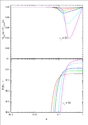
Figure 1: (Color online) The background evolutions. Upper panel: the ratio between the expansion rates in this exponential $f(R)$ cosmology and in $\Lambda\mathrm{CDM}$ as a function of the scale factor $a$. Lower panel: $F(R)-1$ as a function of $a$. The black, red, green, blue, cyan and magenta curves represent cases of $\lambda_{2}=\infty,1000,500,300,100,50$ respectively.

III.2 The TT CMB Spectrum

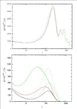
Figure 2: (Color online) Upper panel: The theoretical CMB spectrum of the present model. From bottom to top: $\lambda_{2}=\infty,1000,500$. Lower panel: Contributions from the ISW effect. Solid curves are the results of the $f(R)=R+\lambda_{1}H_{0}^{2}\mathrm{exp}(R/\lambda_{2}H_{0}^{2})$ model, from bottom to top: $\lambda_{2}=\infty,1000,500$; Dashed curves are those of the $f(R)=R+\alpha(-R)^{\beta}$ model for comparison, from bottom to top: $\beta=0,-0.05,-0.1$. In both cases we use $\Omega_{m}=0.3$.

We have calculated the CMB spectrum of the present model using CAMB, with adiabatic initial conditions because the corrections to GR are expected not to influence initial conditions. The results are shown in Fig. 2, where we have plotted the CMB spectra for $\lambda_{2}=\infty,1000$ and 500. Interestingly we see that the deviation from $\Lambda\mathrm{CDM}$ ($\lambda_{2}=\infty$) occurs roughly in the range $l\in(10,500)$, while for even smaller $l$’s it vanishes. This is in contrast to the $f(R)=R+\alpha(-R)^{\beta}$ model, in which drastic changes happen at $l\lesssim 300$ Li (2006). The contributions from ISW effect alone are also shown in Fig. 2, both for the $f(R)=R+\lambda_{1}H_{0}^{2}\mathrm{exp}(R/\lambda_{2}H_{0}^{2})$ and for the $f(R)=R+\alpha(-R)^{\beta}$ models. Obviously these agree qualitatively with the behaviors of the modified CMB spectra in the two models, since at low $l$’s a significant late-time contribution comes from the ISW effect.

The ISW effect involves the integral of the time-variation of the potential weighted by the spherical Bessel functions for each $l$

$$I_{l}^{ISW}(k) = 2\int_{0}^{\eta_{0}}e^{-\tau}\phi^{\prime}_{k}j_{l}[k(\eta_{0}-\eta)]d\eta,$$ (28)

in which $\tau$ is the optical depth, $\eta$ is the conformal time, a prime denotes derivative with respect to $\eta$ and subscript ^′0^′ means the current value; $\phi_{k}$ is Weyl tensor variable defined as the coefficient of harmonic expanding $\mathcal{E}_{ab}$ in terms of $Q^{k}_{ab}$ Lewis (2000)

$$\mathcal{E}_{ab} = -\sum_{k}\frac{k^{2}}{a^{2}}\phi_{k}Q^{k}_{ab},$$ (29)

where $Q^{k}_{ab}=\frac{a^{2}}{k^{2}}\hat{\mathcal{D}}_{\langle a}\hat{\mathcal{D}}_{b\rangle}Q^{k}$ and $Q^{k}$ is the eigenfunction of $\hat{\mathcal{D}}^{2}$ with eigenvalue $k^{2}/a^{2}$.

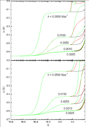
Figure 3: (Color online) Upper panel: The potential $\phi_{k}$ as a function of the scale factor for the different $k$-modes as indicated besides the curves for the $f(R)=R+\lambda_{1}H_{0}^{2}\mathrm{exp}(R/\lambda_{2}H_{0}^{2})$ model. The black, red and green curves represent cases of $\lambda_{2}=\infty,1000$ and 500 respectively. Lower panel: same as above, but for the $f(R)=R+\alpha(-R)^{\beta}$ model, and the black, red and green curves here represent cases of $\beta=0,-0.01$ and -0.05. In both cases we use $\Omega_{m}=0.3$.

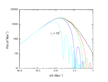
Figure 4: (Color online) The matter power spectrum in the present model. The black, red, green, blue and cyan curves represent the cases of $\lambda_{2}=\infty,10^{5},5\times 10^{4},10^{4}$ and 1000 respectively.

The evolutions of the potential $\phi_{k}$ for various $k$’s are plotted in Fig. 3, and these provide a qualitative explanation for Fig. 2. For the ISW effect, we know that the photons typically travel through many peaks and valleys of the perturbation, and this leads to cancellations of the effects. Mathematically this arises from the oscillatory property of the spherical Bessel function $j_{l}(x)$: $\int dxj_{l}(x)=\sqrt{\pi}\Gamma[\frac{1}{2}(l+1)]/2\Gamma[\frac{1}{2}(l+2)]\approx(\pi/2l)^{1/2}$ Hu (2002). Thus if $\phi^{\prime}_{k}$ is a constant, then $I^{ISW}_{l}(k)$ would roughly scale as $l^{-1/2}$ for a specified $k$. If $\phi^{\prime}_{k}$ is not a constant, on the other hand, it must be weighted by $j_{l}(x)$ at different times in the integration, and, as $j_{l}(x)$ strongly peaks at $x\sim l$, it is weighted more at $x\sim l$ for an $l$. To be more explicit, for the scales we are interested in the ISW integral takes the following form Hu (1995)

$$\int^{\eta_{0}}e^{-\tau}\phi^{\prime}_{k}j_{l}[k(\eta_{0}-\eta)]d\eta\simeq e^{-\tau}\phi^{\prime}_{k}(\eta_{k})\frac{\sqrt{\pi}}{2k}\frac{\Gamma[\frac{1}{2}(l+1)]}{\Gamma[\frac{1}{2}(l+2)]},$$

in which $\eta_{k}=\eta_{0}-(l+1/2)/k$ is the position of the main peak of $j_{l}$.

From Fig. 3 it is clear that $\phi_{k}$ decays rapidly earlier in the $f(R)=R+\lambda_{1}H_{0}^{2}\mathrm{exp}(R/\lambda_{2}H_{0}^{2})$ model than in the $f(R)=R+\alpha(-R)^{\beta}$ model (for such a comparison we could choose $\lambda_{2}$ and $\beta$ such that their endpoints of the evolution paths of $\phi_{k}$ are nearly the same in Fig. 3, e.g., $\lambda_{2}=500$ and $\beta=-0.01$ there). On the other hand, at very late times the evolution of $\phi_{k}$ in the exponential $f(R)$ gravity is nearly the same as in $\Lambda\mathrm{CDM}$. Now consider the contribution from a specified $k$-mode: if $l$ is very large then $\eta_{k}$ will be so small that $\phi^{\prime}_{k}(\eta_{k})\simeq 0$; thus the contribution to this $l$ is negligible. If $l$ is very small, then the contribution to this $l$ will be similar to that in $\Lambda\mathrm{CDM}$ as $\phi^{\prime}_{k}(\eta_{k})\simeq\phi^{\prime}_{k\Lambda\mathrm{CDM}}(\eta_{k})$. For the intermediate $l$’s, since the larger $l$ is the smaller $\eta_{k}$ is, some sufficiently larger $l$’s would receive significant contribution from the ISW effect if the massive decay of the potential occurs earlier (at a time closer to $\eta_{k}$). Qualitatively this is why in Fig. 2 the ISW effect for the $f(R)=R+\lambda_{1}H_{0}^{2}\mathrm{exp}(R/\lambda_{2}H_{0}^{2})$ model extends to larger $l$’s than that of the $f(R)=R+\alpha(-R)^{\beta}$ model and the differences from $\Lambda\text{CDM}$ are reduced dramatically towards very-small $l$’s in the case of exponential $f(R)$ gravity.

As for the CMB polarization spectra of the model, since they are not as sensitive to the parameters as the temperature spectrum, we shall not discuss them here.

III.3 The Matter Power Spectrum

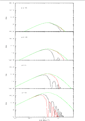
Figure 5: (Color online) The matter power spectra at different redshifts. From bottom to top: $z=0$, $z=5$, $z=10$ and $z=15$. The black, red, and green curves represent the cases of $f(R)=R+\lambda_{1}H_{0}^{2}\mathrm{exp}(R/\lambda_{2}H_{0}^{2})$ ($\lambda_{2}=1000$), $f(R)=R+\alpha(-R)^{\beta}$ ($\beta=-0.01$) and $\Lambda\mathrm{CDM}$ respectively.

As discussed extensively in Koivisto (2006, 2006b), the response of this modified gravity to the spatial variations of matter distribution could be very sensitive (this could also be seen from Eq. (24) above), and at small enough scales this feature would significantly affect the growth of density perturbations. To be explicit, at large enough $k$’s, the growth equation for the comoving energy density fluctuations $\delta_{m}$ could be written as Koivisto (2006)

$$\frac{d^{2}\delta_{m}}{dx^{2}} \doteq -\frac{k^{2}}{H^{2}}\frac{F^{\prime}}{3F(2FH+F^{\prime})}\delta_{m},$$ (30)

in which $x\equiv\log a$ and $F^{\prime}/3F(2FH+F^{\prime})=c_{s}^{2}$ acts as an effective sound speed squared. For the present exponential $f(R)$ theory we have seen from Fig. 1 that $F^{\prime}>0$, so that $c_{s}^{2}>0$ and the small scale density fluctuations will oscillate instead of growing according to Eq. (30). On the other hand, if $c_{s}^{2}<0$, then these small scale fluctuations will become unstable and blow up dramatically Sandvik (2004); this does happen in the $f(R)=R+\alpha(-R)^{\beta}$ model if $\beta$ is positive Li (2006), but not for our choices of parameters in the $f(R)=R+\lambda_{1}H_{0}^{2}\mathrm{exp}(R/\lambda_{2}H_{0}^{2})$ model.

We have also calculated the matter power spectrum in the present model for different choices of $\lambda_{2}$ with the modified CAMB code and the results are shown in Fig. 4. As expected, the matter spectrum is more sensitive to the deviation from GR than the CMB spectrum, because it relates directly to the density perturbations. From this figure we see that $\lambda_{2}\lesssim 5\times 10^{4}$ will hopefully be excluded when tested against the measurements on matter power spectrum from Sloan Digital Sky Survey (SDSS) Tegmark (2004), which is more stringent than the possible CMB constraints.

It will also be interesting to consider when the deviations of the matter power spectrum from the $\Lambda\mathrm{CDM}$ case occur in the $f(R)$ gravity theories. Since $c_{s}^{2}=0$ in the strict $\Lambda\mathrm{CDM}$ model, the deviation will appear when $F^{\prime}$ is significantly nonzero, and it thus appears earlier if $F$ begins to evolve earlier. Fig. 5 confirms this expectation: it is apparent that for the $f(R)=R+\lambda_{1}H_{0}^{2}\mathrm{exp}(R/\lambda_{2}H_{0}^{2})$ model the deviation from the $\Lambda\mathrm{CDM}$ matter power spectrum has almost shaped up before $z\simeq 5$ while for the $f(R)=R+\alpha(-R)^{\beta}$ model this happens much later.

IV Discussion and Conclusions

To summarize, we have investigated the background evolution, CMB and matter power spectra of a class of early $f(R)$ gravity model, which takes the form of $f(R)=R+\lambda_{1}H_{0}^{2}\mathrm{exp}(R/\lambda_{2}H_{0}^{2})$. Such a model has the interesting feature that the deviation from $\Lambda\mathrm{CDM}$ happens only at some intermediate time, and this is why its CMB and matter power spectra are rather different from those in either the $\Lambda\mathrm{CDM}$ case or some late-time $f(R)$ gravity theories, such as $f(R)=R+\alpha(-R)^{\beta}$. For the CMB spectrum, the earlier massive decay of the potential extends the ISW effect to larger $l$’s, leaving the ISW at very low $l$’s indistinguishable from that in $\Lambda\mathrm{CDM}$. Consequently the deviation from the latter is most significant at intermediate $l$’s ($l\in(10,400\sim 500)$), as shown in Fig. 2. For the matter power spectrum, the modifications to GR lead to the appearance of effective pressure fluctuations, which restricts the growths of small-scale density perturbations and leads to oscillations in small scales of the spectrum. It is interesting that, the deviation from $\Lambda\mathrm{CDM}$ matter power spectrum develops rather early in the early $f(R)$ gravity model because $F$ here begins to evolve earlier.

Since the matter power spectrum directly shows the density perturbations while the CMB spectrum does not, the former is more sensitive to corrections to GR in $f(R)$ gravity, as shown in Li (2006). The constraints from local (solar system) measurements plus the SDSS data might be able to restrict the parameter $\lambda_{2}$ into a rather narrow range, roughly $5\sim 10\times 10^{4}\lesssim\lambda_{2}\ll 10^{6}$, but an exact constraint obtainable through carefully searching the parameter space with, say, the Markov Chain Monte Carlo method is beyond the scope of the work here.

The present work therefore contributes to filling in the gap in constraining $f(R)$ corrections to GR at some higher redshifts than when the late-time accelerating expansion of our Universe begins; it shows that such early $f(R)$ cosmologies are strongly disfavored by current data on CMB and matter power spectra, just as their late-time correspondences such as the model $f(R)=R+\alpha(-R)^{\beta}$.