The rest-frame optical luminosity functions of galaxies at $2\leq z\leq 3.5$

Abstract

We present the rest-frame optical ($B$, $V$, and $R$ band) luminosity functions (LFs) of galaxies at $2\leq z\leq 3.5$, measured from a $K$-selected sample constructed from the deep NIR MUSYC, the ultradeep FIRES, and the GOODS-CDFS. This sample is unique for its combination of area and range of luminosities. The faint-end slopes of the LFs at $z>2$ are consistent with those at $z\sim 0$. The characteristic magnitudes are significantly brighter than the local values (e.g., $\sim 1.2$ mag in the $R$ band), while the measured values for $\Phi^{\star}$ are typically $\sim 5$ times smaller. The $B$-band luminosity density at $z\sim 2.3$ is similar to the local value, and in the $R$ band it is $\sim 2$ times smaller than the local value. We present the LF of Distant Red Galaxies (DRGs), which we compare to that of non-DRGs. While DRGs and non-DRGs are characterized by similar LFs at the bright end, the faint-end slope of the non-DRG LF is much steeper than that of DRGs. The contribution of DRGs to the global densities down to the faintest probed luminosities is 14%-25% in number and 22%-33% in luminosity. From the derived rest-frame $U-V$ colors and stellar population synthesis models, we estimate the mass-to-light ratios ($M/L$) of the different subsamples. The $M/L$ ratios of DRGs are $\sim 5$ times higher (in the $R$ and $V$ bands) than those of non-DRGs. The global stellar mass density at $2\leq z\leq 3.5$ appears to be dominated by DRGs, whose contribution is of order $\sim$60%-80% of the global value. Qualitatively similar results are obtained when the population is split by rest-frame $U-V$ color instead of observed $J-K$ color.

1. INTRODUCTION

Understanding the formation mechanisms and evolution with cosmic time of galaxies is one of the major goals of observational cosmology. In the current picture of structure formation, dark matter halos build up in a hierarchical fashion controlled by the nature of the dark matter, the power spectrum of density fluctuations, and the parameters of the cosmological model. The assembly of the stellar content of galaxies is governed by much more complicated physics, such as the mechanisms of star formation, gaseous dissipation, the feedback of stellar and central supermassive black hole energetic output on the baryonic material of the galaxies, and mergers.

The mean space density of galaxies per unit luminosity, or luminosity function (LF), is one of the most fundamental of all cosmological observables, and it is one of the most basic descriptors of a galaxy population. The shape of the LF retains the imprint of galaxy formation and evolution processes; the evolution of the LF as a function of cosmic time, galaxy type and environment provides insights into the physical processes that govern the assembly and the following evolution of galaxies. Therefore, the LF represents one of the fundamental observational tools to constrain the free parameters of theoretical models.

The local ($z\sim 0$) LF has been very well determined from several wide-area, multi-wave band surveys with follow-up spectroscopy (norberg02; blanton01; blanton03; kochanek01; cole01). At intermediate redshifts ($z\sim 0.75$), spectroscopic surveys found a steepening of the faint-end LF with increasing redshift in the global LF, mainly due to the contribution by later type galaxies (lilly95; ellis96). From the COMBO-17 survey, wolf03 measured the rest-frame optical LF up to $z\sim 1.2$, finding that early-type galaxies show a decrease of a factor of $\sim 10$ in the characteristic density $\Phi^{\star}$ of the LF. The latest type galaxies show a brightening of $\sim 1$ mag in $M^{\star}$ (the characteristic magnitude) and an increase of $\sim 1.6$ in $\Phi^{\star}$ in their highest redshift bin in the blue band. Further progress in the measurement of the LF at $z<2$ was obtained with the VIMOS VLT Deep Survey (VVDS; lefevre04) and the DEEP-2 Galaxy Redshift Survey (davis03). From the VVDS data, ilbert05 measured the rest-frame optical LF from $z=0.05$ to $z=2$. From the same data set, zucca06 performed a similar analysis for different spectral galaxy types, finding a significant steepening of the LF going from early to late types. Their results indicate a strong type-dependent evolution of the LF, and identify the latest spectral types as responsible for most of the evolution of the UV-optical LF out to $z=1.5$.

Contrary to low-redshift studies, the selection of high-redshift ($z>2$) galaxies still largely relies on their colors. One of the most efficient ways to select high-redshift galaxies is the Lyman drop-out technique, which enabled Steidel and collaborators to build large samples of $z\sim 3$ star-forming galaxies (steidel96, 1999). Extensive studies of these optically (rest-frame ultraviolet) selected galaxies at $z\sim 3$ (Lyman Break Galaxies [LBGs]) and at $z\sim 2$ (BM/BX galaxies; steidel04; adelberger04) have shown that they are typically characterized by low extinction, modest ages, stellar masses $\sim 10^{10}$ M${}_{\sun}$, and star formation rates of 10–100 M${}_{\sun}$yr${}^{-1}$ (steidel03; shapley01; reddy05). shapley01 recovered the rest-frame $V$-band LF of LBGs at $z\sim 3$ from the rest-frame UV LF (steidel99; but see also sawicki06), finding that the LBG LF is characterized by a very steep faint end.

LBGs dominate the UV luminosity density at $z\sim 2-6$, as well as possibly the global star formation rate density at these redshifts (reddy05). However, since the Lyman break selection technique requires galaxies to be very bright in the rest-frame UV in order to be selected, it might miss galaxies that are heavily obscured by dust or whose light is dominated by evolved stellar populations. These objects can be selected in the near-infrared (NIR), which corresponds to the rest-frame optical out to $z\sim 3$. Using the NIR selection criterion $J-K>2.3$ (also suggested by saracco01), franx03 and vandokkum03 discovered a new population of high-redshift galaxies (distant red galaxies [DRGs]) that would be largely missed by optically selected surveys. Follow-up studies have shown that DRGs constitute a heterogeneous population. They are mostly actively forming stars at $z\sim 1.5-3.5$ (vandokkum03; forster04; rubin04; knudsen05; reddy05; papovich06). However, some show no signs of active star formation and appear to be passively evolving (labbe05; kriek06; reddy06), while others seem to host powerful active galactic nuclei (vandokkum04; papovich06). Compared to LBGs, DRGs have systematically older ages and larger masses (forster04), although some overlap between the two exists (shapley05; reddy05). Recently, vandokkum06 have demonstrated that in a mass-selected sample ($>10^{11}$ $M_{\sun}$) at $2<z<3$, DRGs make up 77% in mass, compared to only 17% from LBGs (see also papovich06), implying that the rest-frame optical LF determined by shapley01 is incomplete.

The global (i.e., including all galaxy types) rest-frame optical LF at $z>2$ can be studied by combining multiwavelength catalogs with photometric redshift information. giallongo05 studied the $B$-band LFs of red and blue galaxies. They find that the $B$-band number densities of red and blue galaxies have different evolution, with a strong decrease of the red population at $z=2-3$ compared to $z=0$ and a corresponding increase of the blue population, in broad agreement with the predictions from their hierarchical cold dark matter models. As all previous works at $z>2$ are based on either very deep photometry but small total survey area (poli03; giallongo05) or larger but still single field surveys (gabasch04), their results are strongly affected by field-to-field variations and by low number statistics, especially at the bright end. Moreover, gabasch04 used an I-band–selected data set from the FORS Deep Field. The $I$ band corresponds to the rest-frame UV at $z\sim 2$, which means that significant extrapolation is required.

In this paper we take advantage of the deep NIR MUSYC survey to measure the rest-frame optical ($B$, $V$, and $R$ band) LFs of galaxies at $2\leq z\leq 3.5$. Its unique combination of surveyed area and depth allows us to (1) minimize the effects of field-to-field variations, (2) better probe the bright end of the LF with good statistics, and (3) sample the LF down to luminosities $\sim 0.9$ mag fainter than the characteristic magnitude. To constrain the faint-end slope of the LF and to increase the statistics, we also made use of the FIRES and the GOODS-CDFS surveys, by constructing a composite sample. The large number of galaxies in our composite sample also allows us to measure the LFs of several subsamples of galaxies, such as DRGs and non-DRGs (defined based on their observed $J-K$ color), and of intrinsically red and blue galaxies (defined based on their rest-frame $U-V$ color).

This paper is structured as follows. In § 2 we present the composite sample used to measure the LF of galaxies at $2\leq z\leq 3.5$; in § 3 we describe the methods applied to measure the LF and discuss the uncertainties in the measured LF due to field-to-field variations and errors in the photometric redshift estimates; the results (of all galaxies and of the individual subsamples considered in this work) are presented in § 4, while the estimates of the number and luminosity densities and the contribution of DRGs (red galaxies) to the global stellar mass density are given in § 5. Our results are summarized in § LABEL:sec-concl. We assume $\Omega_{\rm M}=0.3$, $\Omega_{\rm\Lambda}=0.7$, and $H_{\rm 0}=70$ km s${}^{-1}$ Mpc${}^{-1}$ throughout the paper. All magnitudes and colors are on the Vega system, unless identified as “AB”. Throughout the paper, the $J-K$ color is in the observed frame, while the $U-V$ color refers to the rest frame.

2. THE COMPOSITE SAMPLE

The data set we have used to estimate the LF consists of a composite sample of galaxies built from three deep multiwavelength surveys, all having high-quality optical to NIR photometry: the “ultradeep” Faint InfraRed Extragalactic Survey (FIRES; franx03), the Great Observatories Origins Deep Survey (GOODS; giavalisco04; Chandra Deep Field–South [CDF-S]), and the MUlti-wavelength Survey by Yale-Chile (MUSYC; gawiser06; quadri06). Photometric catalogs were created for all fields in the same way, following the procedures of labbe03.

FIRES consists of two fields, namely, the Hubble Deep Field–South proper (HDF-S) and the field around MS 1054–03, a foreground cluster at $z=0.83$. A complete description of the FIRES observations, reduction procedures, and the construction of photometric catalogs is presented in detail in labbe03 and forster06 for HDF-S and MS 1054–03, respectively. Briefly, the FIRES HDF-S and MS 1054–03 (hereafter FH and FMS, respectively) are $K_{\rm s}$ band–limited multicolor source catalogs down to $K^{\rm tot}_{\rm s}=24.14$ and $K^{\rm tot}_{\rm s}=23.14$, for a total of 833 and 1858 sources over fields of $2.5^{\prime}\times 2.5^{\prime}$ and $5.5^{\prime}\times 5.3^{\prime}$, respectively. The FH and FMS catalogs have 90% completeness level at $K^{\rm tot}_{\rm s}=23.8$ and $K^{\rm tot}_{\rm s}=22.85$, respectively. The final FH (FMS) catalogs used in the construction of the composite sample has 358 (1427) objects over an effective area of 4.74 (21.2) arcmin${}^{2}$, with $K^{\rm tot}_{\rm s}<23.14$ (22.54), which for point sources corresponds to a 10 (8) $\sigma$ signal-to-noise ratio ($S/N$) in the custom isophotal aperture.

Table 1The Composite Sample: Field Specifications

		$K^{\rm tot}_{\rm 90}$	$K^{\rm tot}_{\rm lim,cs}$	Area
Field	Filter Coverage	(mag)	(mag)	(arcmin${}^{2}$)	$N$	$N_{\rm spec}$
FIRES-HDFS	U${}_{\rm 300}$B${}_{\rm 450}$V${}_{\rm 606}$I${}_{\rm 814}$J${}_{\rm s}$HK${}_{\rm s}$	23.80	23.14	4.74	358	68
FIRES-MS1054	UBVV${}_{\rm 606}$I${}_{\rm 814}$J${}_{\rm s}$HK${}_{\rm s}$	22.85	22.54	21.2	1427	297
GOODS-CDFS	B${}_{\rm 435}$V${}_{\rm 606}$i${}_{\rm 775}$z${}_{\rm 850}$JHK${}_{\rm s}$	21.94	21.34	65.6	1588	215
MUSYC	UBVRIzJHK${}_{\rm s}$	21.33	21.09	286.1	5507	116

Note. — $K^{\rm tot}_{\rm 90}$ is the $K_{\rm s}$ band total magnitude 90% completeness limit, $K^{\rm tot}_{\rm lim,cs}$ is the $K_{\rm s}$ band total magnitude limit used to construct the composite sample, $N$ is the total number of sources down to $K^{\rm tot}_{\rm lim,cs}$, and $N_{\rm spec}$ is the number of objects with spectroscopic redshift.

From the GOODS/EIS observations of the CDF-S (data release version 1.0) a $K_{\rm s}$ band limited multicolor source catalog (hereafter CDFS) was constructed, described in S. Wuyts et al. (2007, in preparation). GOODS zero points were adopted for $J$ and $K_{\rm s}$. The $H$-band zero point was obtained by matching the stellar locus on a $J-K$ versus $J-H$ color-color diagram to the stellar locus in FIRES HDF-S and MS 1054–03. The difference with the official GOODS $H$-band zero point varies across the field, but on average our $H$-band zero points are $\sim 0.1$ mag brighter. A total effective area of 65.6 arcmin${}^{2}$ is well exposed in all bands. The final catalog contains 1588 objects with $K^{\rm tot}_{\rm s}<21.34$ in this area. At $K^{\rm tot}_{\rm s}=21.34$ the median $S/N$ in the $K_{\rm s}$ isophotal aperture is $\sim 12$.

MUSYC consists of optical and NIR imaging of four independent $30^{\prime}\times 30^{\prime}$ fields with extensive spectroscopic follow-up (gawiser06). Deeper NIR $JHK_{\rm s}$ imaging was obtained over four $10^{\prime}\times 10^{\prime}$ subfields with the ISPI camera at the Cerro Tololo Inter-American Observatory (CTIO) Blanco 4 m telescope. A complete description of the deep NIR MUSYC observations, reduction procedures, and the construction of photometric catalogs will be presented in quadri06. The 5 $\sigma$ point-source limiting depths are $J\sim 22.9$, $H\sim 21.8$, and $K_{\rm s}\sim 21.3$. The optical $UBVRIz$ data are described in gawiser06. The present work is restricted to three of the four deep fields: the two adjacent fields centered around HDF-S proper (hereafter MH1 and MH2) and the field centered around the quasar SDSS 1030+05 (M1030). The final MUSYC $K_{\rm s}$-selected catalog used in the construction of the composite sample has 5507 objects over an effective area of 286.1 arcmin${}^{2}$, with $K^{\rm tot}_{\rm s}<21.09$, which for point sources corresponds to a $\sim$10 $\sigma$ $S/N$ in the isophotal aperture.

Table 1 summarizes the specifications of each field, including wave band coverage, $K{\rm s}$ band total magnitude 90% completeness limit ($K^{\rm tot}_{\rm 90}$), effective area, the $K{\rm s}$ band total magnitude limit used to construct the composite sample ($K^{\rm tot}_{\rm lim,cs}$), the number of objects, and the number of sources with spectroscopic redshifts.

Only a few percent of the sources in the considered catalogs have spectroscopic redshift measurements. Consequently, we must rely primarily on photometric redshift estimates. Photometric redshifts $z_{\rm phot}$ for all galaxies are derived using an identical code to that presented in rudnick01; rudnick03, but with a slightly modified template set. This code models the observed spectral energy distribution (SED) using nonnegative linear combinations of a set of eight galaxy templates. As in rudnick03, we use the E, Sbc, Scd, and Im SEDs from coleman80, the two least reddened starburst templates from kinney96, and a synthetic template corresponding to a 10 Myr old simple stellar population (SSP) with a salpeter55 stellar initial mass function (IMF). We also added a 1 Gyr old SSP with a Salpeter IMF, generated with the bruzual03 evolutionary synthesis code. The empirical templates have been extended into the UV and the NIR using models. Comparing the photometric redshifts with 696 spectroscopic redshifts (63 at $z\geqslant 1.5$) collected from the literature and from our own observations gives a scatter in $\Delta z/(1+z)$ of $\sigma=0.06$. Restricting the analysis to galaxies at $z\geqslant 1.5$ in the MUSYC fields gives $\sigma=0.12$, corresponding to $\Delta z\approx 0.4$ at $z=2.5$. Approximately 5% of galaxies in this sample are “catastrophic” outliers. A full discussion of the quality of the photometric redshifts is given elsewhere (quadri06). The effects of photometric redshift errors on the derived LFs are modeled in § 3.3.

Rest-frame luminosities are computed from the observed SEDs and redshift information using the method extensively described in the Appendix of rudnick03. This method does not depend directly on template fits to the data but rather interpolates directly between the observed fluxes, using the best-fit templates as a guide. We computed rest-frame luminosities in the $U$, $B$, $V$, and $R$ filters of bessell90. For these filters we use $M_{\rm\sun,U}=+5.66$, $M_{\rm\sun,B}=+5.47$, $M_{\rm\sun,V}=+4.82$, and $M_{\rm\sun,R}=+4.28$. In all cases where a spectroscopic redshift is available we computed the rest-frame luminosities fixed at $z_{\rm spec}$.

Stars in all $K_{\rm s}$-selected catalogs were identified by spectroscopy, by fitting the object SEDs with stellar templates from hauschildt99 and/or inspecting their morphologies, as in rudnick03. On average, approximately 10% of all the objects were classified as stars.

We constructed a composite sample of high-redshift ($2\leq z\leq 3.5$) galaxies to be used in the estimate of the LF in § 3. A large composite sample with a wide range of luminosities is required to sample both the faint and the bright end of the LF well; moreover, a large surveyed area is necessary to account for sample variance. The very deep FIRES allows us to constrain the faint end of the LF, while the large area of MUSYC allows us to sample the bright end of the LF very well. The CDFS catalog bridges the two slightly overlapping regimes and improves the number statistics. The final composite sample includes 442, 405, and 547 $K_{\rm s}$-selected galaxies in the three targeted redshift intervals $2\leq z\leq 2.5$, $2.7\leq z\leq 3.3$, and $2.5<z\leq 3.5$, respectively, for a total of 989 galaxies with $K_{\rm s}^{\rm tot}<23.14$ at $2\leq z\leq 3.5$. Of these, $\sim$4% have spectroscopic redshifts. In Figure 1 we show the rest-frame $B$-band absolute magnitude versus the redshift for the composite sample in the studied redshift range $2\leq z\leq 3.5$.

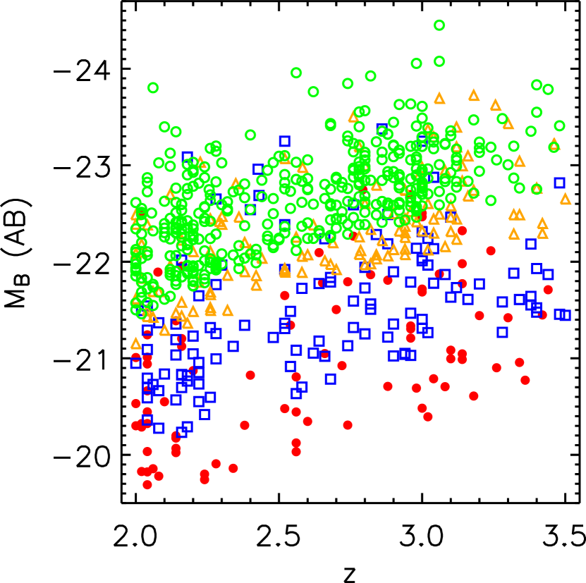
Figure 1.— Rest-frame $B$-band magnitude vs. redshift for the composite sample in the redshift range $2\leq z\leq 3.5$; the FH, FMS, CDFS, and MUSYC fields are plotted as red filled circles, blue open squares, orange open triangles, and green open circles, respectively.

3. METHODOLOGY

3.1. The $1/V_{\rm max}$ Method

To estimate the observed LF in the case of a composite sample, we have applied an extended version of the $1/V_{\rm max}$ algorithm (schmidt68) as defined in avni80 so that several samples can be combined in one calculation. For a given redshift interval [$z_{\rm 1}$,$z_{\rm 2}$], we computed the galaxy number density $\Phi(M)$ in each magnitude bin $\Delta M$ in the following way:

$$\Phi(M)=\frac{1}{\Delta M}\sum_{i=1}^{N}{\frac{1}{V_{\rm i}}},$$ (1)

where $N$ is the number of objects in the chosen bin and $V_{\rm i}$ is:

$$V_{\rm i}=\sum_{j=1}^{n}{\omega_{\rm j}\int_{z_{\rm min}}^{z_{\rm up}(i,j)}{\frac{dV}{dz}dz}},$$ (2)

where $\omega_{\rm j}$ is the area in units of steradians corresponding to the $j$th field, $n$ is the number of samples combined together, $dV/dz$ is the comoving volume element per steradian, and $z_{\rm up}(i,j)$ is the minimum of $z_{\rm 2}$ and the maximum redshift at which the $i$th object could have been observed within the magnitude limit of the $j$th sample. The Poisson error in each magnitude bin was computed adopting the recipe of gehrels86 valid also for small numbers.

The $1/V_{\rm max}$ estimator has the advantages of simplicity and no a priori assumption of a functional form for the luminosity distribution; it also yields a fully normalized solution. However, it can be affected by the presence of clustering in the sample, leading to a poor estimate of the faint-end slope of the LF. Although field-to-field variation represents a significant source of uncertainty in deep surveys (since they are characterized by very small areas and hence small sampled volumes), the majority of published cosmological number densities and related quantities do not properly account for sample variance in their quoted error budgets. Our composite sample is made of several independent fields with a large total effective area of $\sim 380$ arcmin${}^{2}$ (about a factor of 3 larger than the nominal area of the $K_{\rm s}$-selected CDFS-GOODS catalog used in dahlen05), which significantly reduces the uncertainties due to sample variance. Also, the large number of fields considered in this work with their large individual areas allows us to empirically measure the field-to-field variations from one field to the other in the estimate of the LF with the $1/V_{\rm max}$ method, especially at the bright end, and to properly account for it in the error budget.

In order to quantify the uncertainties due to field-to-field variations in the determination of the LF, we proceeded as follows. First, for each magnitude bin $\Delta M$, we measured $\Phi^{\rm j}$ for each individual $j$th field using equation (1). For each magnitude bin with $n\geqslant 3$, we estimated the contribution to the error budget of $\Phi(M)$ from sample variance using:

$$\sigma_{\rm sv}=\frac{rms(\Phi^{\rm j})}{\sqrt{n}},$$ (3)

with $n$ the number of individual fields used. For the magnitude bins with $n\leqslant 2$ (usually the brightest bin and the 3-4 faintest ones), we adopted the mean of the $rms(\Phi^{\rm j})$ with $n\geqslant 3$. The final 1 $\sigma$ error associated to $\Phi(M)$ is then $\sigma=(\sigma_{\rm Poi}^{2}+\sigma_{\rm sv}^{2})^{1/2}$, with $\sigma_{\rm Poi}$ the Poisson error in each magnitude bin.

3.2. The Maximum Likelihood Method

We also measured the observed LF using the STY method (sandage79), which is a parametric maximum likelihood estimator. The STY method has been shown to be unbiased with respect to density inhomogeneities (e.g., efstathiou88), it has well-defined asymptotic error properties (e.g. kendall61), and does not require binning of the data. The STY method assumes that $\Phi(M)$ has a universal form, i.e., the number density of galaxies is separable into a function of luminosity times a function of position: $n(M,{\bf x})=\Phi(M)\rho({\bf x})$. Therefore, the shape of $\Phi(M)$ is determined independently of its normalization. We have assumed that $\Phi(M)$ is described by a schechter76 function,

$$\Phi(M)=(0.4\ln{10})\Phi^{\star}\big{[}10^{0.4(M^{\star}-M)(1+\alpha)}\big{]}{}$$

$$\times\exp{\big{[}-10^{0.4(M^{\star}-M)}\big{]}},$$ (4)

where $\alpha$ is the faint-end slope parameter, $M^{\star}$ is the characteristic absolute magnitude at which the LF exhibits a rapid change in the slope, and $\Phi^{\star}$ is the normalization.

The probability of seeing a galaxy of absolute magnitude $M_{\rm i}$ at redshift $z_{\rm i}$ in a magnitude-limited catalog is given by

$$p_{\rm i}\propto\frac{\Phi(M_{\rm i})}{\int_{M_{\rm faint}(z_{\rm i})}^{M_{\rm bright}(z_{\rm i})}{\Phi(M)dM}},$$ (5)

where $M_{\rm faint}(z_{\rm i})$ and $M_{\rm bright}(z_{\rm i})$ are the faintest and brightest absolute magnitudes observable at the redshift $z_{\rm i}$ in a magnitude-limited sample. The likelihood $\Lambda=\prod_{i=1}^{N}{p_{\rm i}}$ (where the product extends over all galaxies in the sample) is maximized with respect to the parameters $\alpha$ and $M^{\star}$ describing the LF $\Phi(M)$. The best-fit solution is obtained by minimizing $-2\ln{\Lambda}$. A simple and accurate method of estimating errors is to determine the ellipsoid of parameter values defined by

$$\ln{\Lambda}=\ln{\Lambda_{\rm max}}-\frac{1}{2}\chi^{2}_{\rm\beta}(S),$$ (6)

where $\chi^{2}_{\rm\beta}(S)$ is the $\beta$-point of the $\chi^{2}$ distribution with $S$ degrees of freedom. Parameter $\chi^{2}_{\rm\beta}(S)$ is chosen in the standard way depending on the desired confidence level in the estimate (as described, e.g., by avni76; lampton76): $\chi^{2}_{\rm\beta}(2)=2.3$, 6.2, and 11.8 to estimate $\alpha-M^{\star}$ error contours with 68%, 95%, and 99% confidence level (1, 2, and 3 $\sigma$, respectively). The value of $\Phi^{\star}$ is then obtained by imposing a normalization on the best-fit LF such that the total number of observed galaxies in the composite sample is reproduced. The 1, 2, and 3 $\sigma$ errors on $\Phi^{\star}$ are estimated from the minimum and maximum values of $\Phi^{\star}$ allowed by the 1, 2, and 3 $\sigma$ confidence contours in the $\alpha-M^{\star}$ parameter space, respectively.

3.3. Uncertainties due to Photometric Redshift Errors

Studies of high-redshift galaxies still largely rely on photometric redshift estimates. It is therefore important to understand how the photometric redshift uncertainties affect the derived LF and to quantify the systematic effects on the LF best-fit parameters.

chen03 have shown that at lower redshifts ($z\lesssim 1$) the measurement of the LF is strongly affected by errors associated with $z_{phot}$. Specifically, large redshift errors together with the steep slope at the bright end of the galaxy LF tend to flatten the observed LF and result in measured $M^{\star}$ systematically brighter than the intrinsic value, since there are more intrinsically faint galaxies scattered into the bright end of the LF than intrinsically bright galaxies scattered into the faint end. Using Monte Carlo simulations, chen03 obtained a best-fit $M^{\star}$ that was 0.8 mag brighter than the intrinsic value in the redshift range $0.5\leq z\leq 0.8$.

In order to quantify the systematic effect on the LF parameters $\alpha$ and $M^{\star}$ in our redshift range of interest ($2\leq z\leq 3.5$), we performed a series of Monte Carlo simulations. The details of these simulations and the results are presented in Appendix LABEL:app-1. Briefly, we generated several model catalogs of galaxies of different brightness according to an input Schechter LF, extracted the redshifts of the objects from a probability distribution proportional to the comoving volume per unit redshift ($dV/dz$), and obtained the final mock catalogs after applying a limit in the observed apparent magnitude. To simulate the errors in the redshifts, we assumed a redshift error function parametrized as a Gaussian distribution function of 1 $\sigma$ width $\sigma^{\prime}_{\rm z}(1+z)$, with $\sigma^{\prime}_{\rm z}$ being the scatter in $\Delta z/(1+z_{\rm spec})$, and we formed the observed redshift catalog by perturbing the input galaxy redshift within the redshift error function. Finally, we determined the LF for the galaxies at $z_{1}\leq z\leq z_{2}$ using the $1/V_{\rm max}$ and maximum likelihood methods described in §§ 3.1 and 3.2, respectively. As shown in Appendix LABEL:app-1, the systematic effects on the measured $\alpha$ and $M^{\star}$ in the redshift interval $2\leq z\leq 3.5$ are negligible with respect to the other uncertainties in the LF estimate if the errors on the photometric redshifts are characterized by a scatter in $\Delta z/(1+z_{\rm spec})$ of $\sigma^{\prime}_{\rm z}\sim 0.12$, which is the appropriate value for the $z\geq 2$ sample considered in this work. This is not true at $z<1$, where we find large systematic effects on both $M^{\star}$ and $\alpha$, consistent with chen03. As explained in detail in Appendix LABEL:app-1, the large systematic effects found at $z<1$ arise from the strong redshift dependency of both $dV/dz$ and $dM/dz$ at low-$z$; at $z>2$ these dependencies are much less steep, and this results in smaller systematic effects on the measured LF. From the Monte Carlo simulations we also quantified that the effects of photometric redshift errors on the estimated luminosity density are typically a few percent (always $<6$%).

We conclude that the parameters of the LF and the luminosity density estimates presented in this work are not significantly affected by the uncertainties in the photometric redshift estimates. In order to include this contribution in the error budget, we conservatively assume a 10% error contribution to the luminosity density error budget due to uncertainties in the photometric redshift estimates.

4. THE OBSERVED LUMINOSITY FUNCTIONS

In this section we present the results of the measurement of the LF of galaxies at $z\geq 2$. We have measured the global LF in the rest-frame $R$ and $V$ band at redshift $2\leq z\leq 2.5$ and $2.7\leq z\leq 3.3$, respectively. As shown in Figure 2, at these redshifts, the rest-frame $R$ and $V$ bands correspond approximately to the observed $K_{\rm s}$ band, which is the selection band of the composite sample. We also measured the global LF in the rest-frame $B$ band in the redshift interval $2\leq z\leq 2.5$, to compare it with the rest-frame $R$-band LF, and at redshift $2.5<z\leq 3.5$, to compare it with previous studies. For each redshift interval and rest-frame band we also split the sample based on the observed $J-K$ color ($J-K>2.3$, DRGs; $J-K\leq 2.3$, non-DRGs) and the rest-frame $U-V$ color ($U-V\geq 0.25$, red galaxies; $U-V<0.25$, blue galaxies). In § 4.1 we present the global LF of all galaxies, and in § 4.2 we present the LFs of the considered subsamples (DRGs, non-DRGs, red and blue galaxies) in the rest-frame $R$ band. The results for the rest-frame $V$ and $B$ bands are shown in Appendix LABEL:app-2; in Appendix LABEL:app-3 we compare our results with those in the literature.

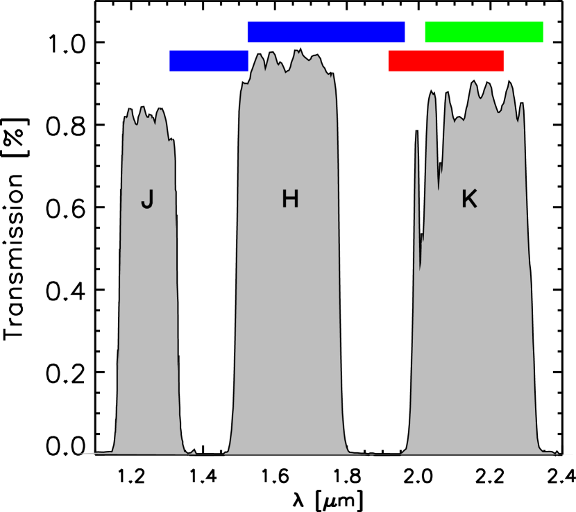
Figure 2.— Transmission curves of the $J$, $H$, and $K_{\rm s}$ bands (gray shaded regions). The filled rectangles represent the observed wavelength ranges spanned by the central wavelengths of the rest-frame $R$ band at $2\leq z\leq 2.5$ (red), of the rest-frame $V$ band at $2.7\leq z\leq 3.3$ (green), and of the rest-frame $B$ band at $2\leq z\leq 2.5$ and $2.5<z\leq 3.5$ (blue; lower and upper rectangles, respectively). For the considered redshift intervals, the rest-frame $R$ and $V$ bands correspond approximately to the observed $K_{\rm s}$ band.

4.1. Rest-Frame LF of All Galaxies

Figure 3 shows the global rest-frame $R$- and $B$-band LFs for galaxies at $2\leq z\leq 2.5$, the rest-frame $V$-band LF at $2.7\leq z\leq 3.3$, and the rest-frame $B$-band LF at $2.5<z\leq 3.5$. The large surveyed area of the composite sample allows the determination of the bright end of the optical LF at $z\geq 2$ with unprecedented accuracy, while the depth of FIRES allows us to constrain also the faint-end slope. This is particularly important because of the well-known correlation between the two parameters $\alpha$ and $M^{\star}$. The best-fit parameters with their 1, 2 and 3 $\sigma$ errors (from the maximum likelihood analysis) are listed in Table 2, together with the Schechter parameters of the local rest-frame $R$-band (from blanton03) and $B$-band (from norberg02) LFs.

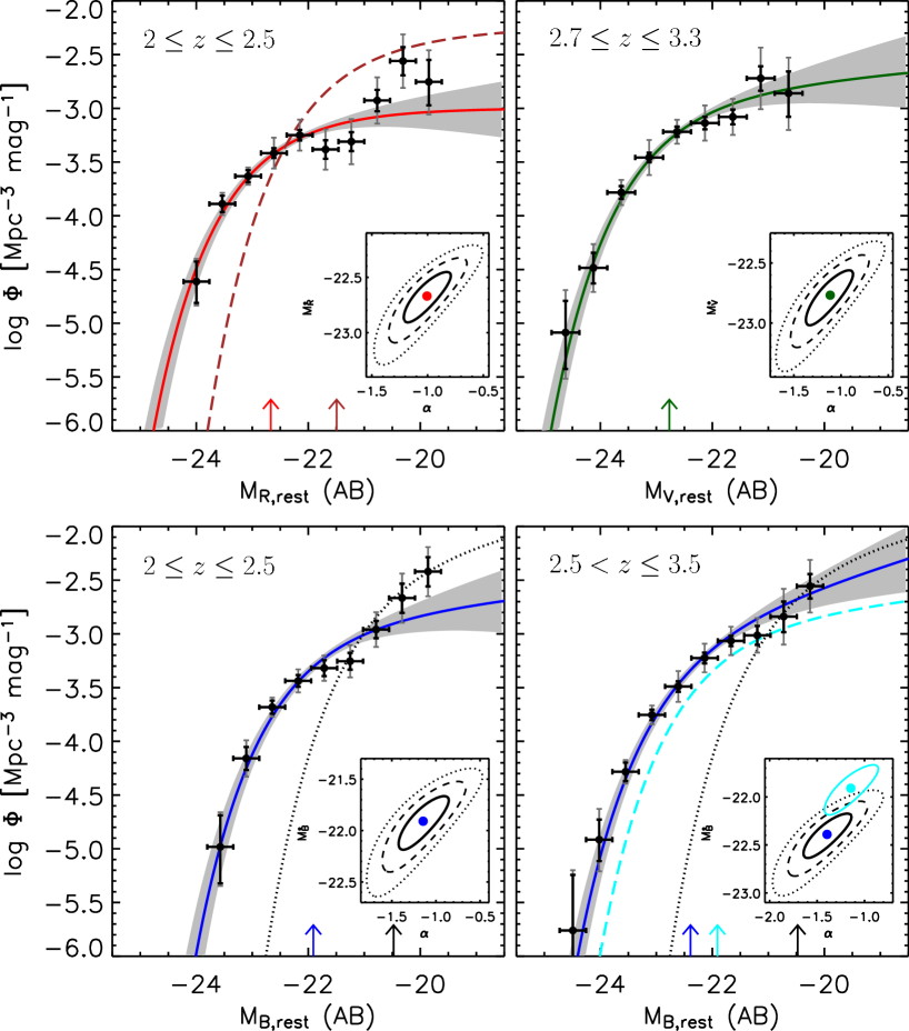
Figure 3.— Top left: Rest-frame $R$-band LF at $2\leq z\leq 2.5$ for all galaxies; black filled circles are the $1/V_{\rm max}$ method estimates with 1 $\sigma$ error bars (Poisson errors only in black; field-to-field variation term included in gray); the red solid line is the LF estimated from the maximum likelihood method, and the red arrow represents the best-fit $M^{\star}$; the shaded region represents the 1 $\sigma$ uncertainties of the LF estimated from the maximum likelihood method; the brown dashed line and arrow represent the local $R$-band LF from SDSS (blanton03; $R=r-0.12$); the inset shows the best-fit value and the 1, 2, and 3 $\sigma$ confidence contour levels of the two parameters $\alpha$ and $M^{\star}$. Top right: Rest-frame $V$-band global LF at $2.7\leq z\leq 3.3$; the dark green solid line and the arrow represent the LF from the maximum likelihood method. Bottom left: Rest-frame $B$-band global LF at $2\leq z\leq 2.5$; the blue solid line and the arrow represent the LF from the maximum likelihood method; the black dotted line and arrow represent the local $B$-band LF from the 2dFGRS (norberg02; $B=b_{\rm J}+0.12$). Bottom right: Rest-frame $B$-band global LF at $2.5<z\leq 3.5$; the cyan dashed line and arrow represent the rest-frame $B$-band LF of all galaxies at $2\leq z\leq 2.5$ for comparison; the black dotted line and arrow represent the local $B$-band LF from the 2dFGRS; in the inset, the 1 $\sigma$ confidence level of the estimated rest-frame $B$-band LF at $2\leq z\leq 2.5$ is also plotted.

Table 2Best-fit Schechter Function Parameters for the Global LFs

		$M^{\star}$		$\Phi^{\star}$
Redshift Range	Rest-Frame Band	(AB)	$\alpha$	(10${}^{-4}$ Mpc${}^{-3}$ mag${}^{-1}$)
$2.0\leq z\leq 2.5$	$R$	$-22.67^{+0.20,0.35,0.45}_{-0.22,0.41,0.61}$	$-1.01^{+0.21,0.35,0.49}_{-0.20,0.34,0.47}$	$10.65^{+2.65,4.50,5.92}_{-2.67,4.40,5.93}$
$z=0$	$R$	$-21.50\pm 0.01$	$-1.05\pm 0.01$	$51.1\pm 1.4$
$2.7\leq z\leq 3.3$	$V$	$-22.77^{+0.20,0.33,0.45}_{-0.24,0.43,0.63}$	$-1.12^{+0.23,0.40,0.57}_{-0.25,0.41,0.57}$	$15.07^{+4.12,6.84,9.45}_{-4.41,7.03,9.28}$
$2.0\leq z\leq 2.5$	$B$	$-21.91^{+0.22,0.39,0.51}_{-0.26,0.49,0.73}$	$-1.15^{+0.28,0.48,0.66}_{-0.27,0.45,0.63}$	$14.57^{+4.60,8.07,11.07}_{-4.64,7.53,9.84}$
$2.5<z\leq 3.5$	$B$	$-22.39^{+0.20,0.35,0.45}_{-0.24,0.43,0.63}$	$-1.40^{+0.25,0.42,0.58}_{-0.24,0.41,0.56}$	$13.56^{+4.69,8.38,11.49}_{-4.51,7.08,9.17}$
$z=0$	$B$	$-20.48\pm 0.07$	$-1.24\pm 0.03$	$62.9\pm 3.1$

Note. — The quoted errors correspond to the 1, 2, and 3 $\sigma$ errors estimated from the maximum likelihood analysis as described in § 3.2. The $z=0$ values are the Schechter parameters of the local rest-frame $R$-band (from blanton03) and $B$-band (from norberg02) LFs. We assumed $R_{\rm AB}=r-0.12$ and $B_{\rm AB}=b_{\rm J}+0.12$ to convert the local values into our photometric system.

At redshift $2\leq z\leq 2.5$, the faint-end slope of the rest-frame $R$-band LF is slightly flatter than in the rest-frame $B$-band, although the difference is within the errors. In the two higher redshift bins, the faint-end slope of the rest-frame $V$-band LF is flatter (by $\sim 0.3$) than in the rest-frame $B$-band, although the difference is only at the 1 $\sigma$ level. Similarly, the faint-end slopes of the rest-frame $B$-band global LF in the low- and high-redshift bins are statistically identical. The characteristic magnitude $M^{\star}_{\rm B}$ in the low-$z$ interval is about 0.5 mag fainter with respect to the high-redshift one, although the difference is significant only at the $\sim$1.5 $\sigma$ level. We therefore conclude that the rest-frame $B$-band global LFs in the low- and high-redshift bins are consistent with no evolution within their errors ($<2$ $\sigma$).

In Figure 3 we have also plotted the local ($z\sim 0.1$) rest-frame $R$-band (from blanton03) and $B$-band (from norberg02) LFs. The faint-end slope of the $R$-band LF at $2\leq z\leq 2.5$ is very similar to the faint-end slope of the local LF; the characteristic magnitude is instead significantly ($>3$ $\sigma$) brighter than the local value (by $\sim 1.2$ mag), and the characteristic density is a factor of $\sim 4.8$ smaller than the local value. The rest-frame $B$-band LF at $2.5<z\leq 3.5$ is characterized by a faint-end slope consistent with the local $B$-band LF; the characteristic magnitude is significantly brighter ($>3$ $\sigma$) than the local value by $\sim 1.9$ mag, while the characteristic density is a factor of $\sim 4.6$ smaller with respect to the local value.

4.2. Rest-Frame LF of DRGs, Non-DRGs, and Red and Blue Galaxies

In this section we present the results of the LFs for different subsamples, by splitting the composite sample based on the observed $J-K$ color ($J-K>2.3$, DRGs; franx03) and on the rest-frame $U-V$ color (by defining the red galaxies as those having $U-V\geq 0.25$, which is the median value of $U-V$ of the composite sample at $2\leq z\leq 2.5$). In Figure 4, we show the rest-frame $U-V$ color versus the observed $J-K$ color for the composite sample at $2\leq z\leq 3.5$.

Figure 4.— Rest-frame $U-V$ color vs. observed $J-K$ color for the composite sample at $2\leq z\leq 3.5$; the dashed vertical line represents the $J-K>2.3$ selection of DRGs, while the horizontal dashed line shows the $U-V\geq 0.25$ definition of red galaxies adopted in this paper.

In Figure 5 we show the rest-frame $R$-band LF at $2\leq z\leq 2.5$ of DRGs versus non-DRGs and red versus blue galaxies, together with the 1, 2, and 3 $\sigma$ contour levels in the $\alpha-M^{\star}_{\rm R,AB}$ parameter space from the STY analysis. The LFs of the different subsamples in the rest-frame $V$ band at $2.7\leq z\leq 3.3$ and in the rest-frame $B$ band at $2\leq z\leq 2.5$ and $2.5<z\leq 3.5$ are shown in Appendix LABEL:app-2 in Figures. LABEL:LF_V_highz.ps, LABEL:LF_B_lowz.ps, and LABEL:LF_B_highz.ps, respectively. In Table 3 the best-fit parameters and their 1, 2, and 3 $\sigma$ errors from the STY method are listed for all the considered rest-frame bands and redshift intervals.

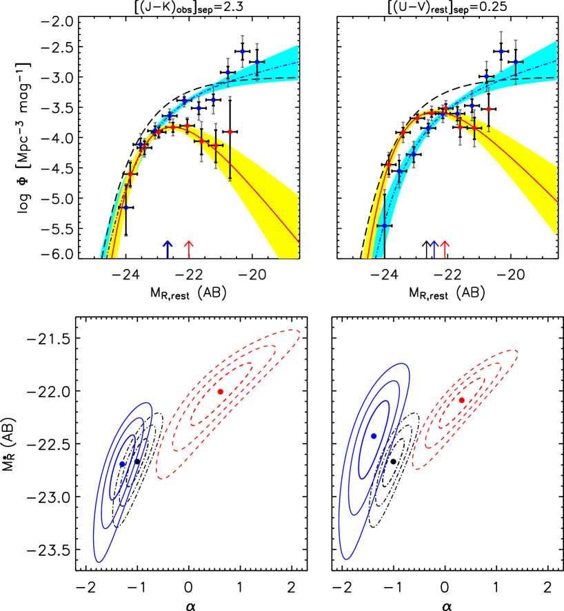
Figure 5.— Rest-frame R-band LF at $2\leq z\leq 2.5$. Top: Rest-frame $R$-band LFs at $2\leq z\leq 2.5$ for DRGs/non-DRGs (left) and red/blue galaxies (right). The red solid line and filled circles represent the LF of DRGs and red galaxies estimated with the STY and $1/V_{\rm max}$ methods, respectively; the blue dot-dashed line and filled circles represent the LF of non-DRGs and blue galaxies. The rest-frame $R$-band LF of all galaxies is also plotted (black dashed line). The shaded region (yellow for DRGs/red galaxies, cyan for non-DRGs/blue galaxies) represents the 1 $\sigma$ uncertainties of the LF measured with the STY method. The arrows represent the best-fit $M^{\star}$; error bars as in Fig. 3. Bottom: 1, 2, and 3 $\sigma$ contour levels from the STY method for DRGs and red galaxies (red dashed lines), for non-DRGs and blue galaxies (blue solid lines), and for all galaxies (black dot-dashed lines); the filled circles represent the best-fit Schechter values. The LF of non-DRGs (blue galaxies) is steeper than that of DRGs (red galaxies).

Table 3Best-Fit Schechter Function Parameters for Subsamples

			$M^{\star}$		$\Phi^{\star}$
Redshift Range	Rest-Frame Band	Sample	(AB)	$\alpha$	(10${}^{-4}$ Mpc${}^{-3}$ mag${}^{-1}$)
$2.0\leq z\leq 2.5$	$R$	$J-K>2.3$	$-22.01^{+0.26,0.43,0.57}_{-0.30,0.55,0.81}$	$0.62^{+0.62,1.07,1.54}_{-0.57,0.92,1.24}$	$3.74^{+0.69,1.02,1.37}_{-1.09,1.90,2.58}$
		$J-K\leq 2.3$	$-22.69^{+0.27,0.43,0.57}_{-0.33,0.60,0.93}$	$-1.30^{+0.24,0.41,0.57}_{-0.24,0.40,0.55}$	$6.32^{+2.72,4.59,6.30}_{-2.41,3.76,4.78}$
		$U-V\geq 0.25$	$-22.09^{+0.20,0.35,0.47}_{-0.24,0.45,0.65}$	$0.33^{+0.43,0.76,1.09}_{-0.44,0.70,0.95}$	$7.51^{+0.69,1.14,1.57}_{-1.14,2.19,3.31}$
		$U-V<0.25$	$-22.43^{+0.32,0.51,0.69}_{-0.40,0.75,1.15}$	$-1.39^{+0.29,0.49,0.68}_{-0.29,0.48,0.67}$	$5.26^{+2.97,4.97,7.32}_{-2.42,3.64,4.47}$
$2.7\leq z\leq 3.3$	$V$	$J-K>2.3$	$-22.63^{+0.28,0.47,0.63}_{-0.36,0.65,0.99}$	$-0.46^{+0.52,0.89,1.27}_{-0.49,0.81,1.10}$	$6.14^{+1.10,1.81,2.56}_{-1.71,3.09,4.34}$
		$J-K\leq 2.3$	$-22.63^{+0.24,0.41,0.55}_{-0.32,0.57,0.87}$	$-1.21^{+0.30,0.50,0.71}_{-0.31,0.50,0.69}$	$11.14^{+4.02,7.12,9.88}_{-4.27,6.61,8.41}$
		$U-V\geq 0.25$	$-22.43^{+0.28,0.45,0.61}_{-0.32,0.59,0.87}$	$-0.11^{+0.60,1.02,1.46}_{-0.53,0.87,1.19}$	$6.25^{+0.87,1.54,2.24}_{-0.92,2.08,3.40}$
		$U-V<0.25$	$-22.65^{+0.26,0.43,0.57}_{-0.30,0.57,0.85}$	$-1.26^{+0.31,0.51,0.73}_{-0.29,0.49,0.68}$	$11.01^{+4.50,7.72,10.55}_{-4.16,6.52,8.36}$
$2.0\leq z\leq 2.5$	$B$	$J-K>2.3$	$-21.75^{+0.42,0.67,0.87}_{-0.54,1.03,1.73}$	$-0.54^{+0.73,1.25,1.79}_{-0.66,1.08,1.47}$	$4.12^{+1.29,2.18,3.18}_{-1.77,2.99,3.78}$
		$J-K\leq 2.3$	$-21.89^{+0.26,0.43,0.57}_{-0.32,0.59,0.89}$	$-1.25^{+0.31,0.53,0.73}_{-0.31,0.52,0.72}$	$11.08^{+4.52,7.83,10.92}_{-4.36,6.75,8.57}$
		$U-V\geq 0.25$	$-21.63^{+0.30,0.49,0.65}_{-0.38,0.69,1.05}$	$-0.40^{+0.57,0.99,1.41}_{-0.56,0.91,1.24}$	$8.63^{+1.57,2.70,3.95}_{-2.33,4.35,6.20}$
		$U-V<0.25$	$-21.83^{+0.32,0.51,0.67}_{-0.42,0.77,1.19}$	$-1.33^{+0.34,0.58,0.81}_{-0.35,0.58,0.81}$	$8.19^{+4.47,7.70,10.97}_{-3.94,5.83,7.09}$
$2.5<z\leq 3.5$	$B$	$J-K>2.3$	$-22.35^{+0.32,0.51,0.67}_{-0.38,0.73,1.17}$	$-1.11^{+0.51,0.86,1.21}_{-0.49,0.81,1.14}$	$4.88^{+2.09,3.35,4.55}_{-2.20,3.48,4.32}$
		$J-K\leq 2.3$	$-22.35^{+0.26,0.43,0.57}_{-0.30,0.57,0.87}$	$-1.45^{+0.30,0.51,0.71}_{-0.29,0.48,0.67}$	$9.50^{+4.53,7.95,11.13}_{-3.92,6.04,7.57}$
		$U-V\geq 0.25$	$-22.25^{+0.32,0.51,0.67}_{-0.38,0.75,1.17}$	$-1.01^{+0.55,0.92,1.31}_{-0.52,0.87,1.21}$	$5.37^{+2.05,3.25,4.49}_{-2.34,3.77,4.73}$
		$U-V<0.25$	$-22.41^{+0.26,0.43,0.57}_{-0.30,0.57,0.87}$	$-1.49^{+0.30,0.50,0.70}_{-0.27,0.47,0.65}$	$8.80^{+4.33,7.60,10.84}_{-3.64,5.62,7.00}$

Note. — The quoted errors correspond to the 1, 2, and 3 $\sigma$ errors estimated from the maximum likelihood analysis as described in § 3.2.

As shown in Figure 5, the rest-frame $R$-band LF at $2\leq z\leq 2.5$ of DRGs is significantly ($>3$ $\sigma$) different from that of non-DRGs. The faint-end slope of the non-DRG LF is much steeper, indicating that the contribution of DRGs to the global luminosity and number density at faint luminosities is very small compared to that of non-DRGs. The bright end of the DRG LF is instead very similar to that of non-DRGs, with the two subsamples contributing equally to the global LF. Splitting the composite sample based on the rest-frame $U-V$ color, we find a qualitatively similar result, with the faint-end slope of the blue galaxy LF being much steeper than that of red galaxies (although the red galaxies clearly dominate the bright end of the LF). The difference between the LFs of DRGs (red galaxies) and non-DRGs (blue galaxies) is mainly driven by the different faint-end slopes.

A similar result holds in the rest-frame $V$ band at $2.7\leq z\leq 3.3$, although it is slightly less significant (at the 2-3 $\sigma$ level): the non-DRG (blue galaxy) LF is very similar to that of DRGs (red galaxies) at the bright end, while at the faint end, the LF of non-DRGs (blue galaxies) is steeper than that of DRGs (red galaxies). In the rest-frame $B$ band, the differences between the LFs of DRGs/red galaxies and non-DRGs/blue galaxies become even less significant. Although DRGs/red galaxies are always characterized by LFs with flatter faint-end slopes, the significance of this result is only marginal ($<2$ $\sigma$), especially in the higher redshift interval.

Within our sample, there is marginal evidence for evolution with redshift: the rest-frame $B$-band non-DRG/blue galaxy LFs in the two targeted redshift bins are characterized by similar (within the errors) faint-end slopes, while the characteristic magnitude is brighter by $\sim 0.5-0.6$ mag in the higher redshift bin. The LF of DRGs/red galaxies tends to get steeper from low to high redshifts and $M^{\star}$ gets brighter by $\sim 0.6$ mag. However, because of the large uncertainties (especially for DRGs and red galaxies) on the measured Schechter parameters, the differences in the rest-frame $B$ band between the high- and the low-redshift bins are at most at the 2 $\sigma$ significance level.

We note that the uncertainties on the estimated Schechter parameters mainly arise from the small number statistics at the very faint end, which is probed only by FIRES. Very deep (down to the deepest FIRES) NIR imaging over large spatially disjoint fields is required for further progress in our understanding of the lowest luminosity galaxies at $z>2$.

4.3. Comparison with LBGs

shapley01 computed the rest-frame optical ($V$ band) LF of $z\sim 3$ LBGs using the distribution of optical $\cal{R}$ magnitudes (i.e., the rest-frame UV LF) and the distribution of $\cal{R}$-$K_{\rm s}$ colors as a function of $\cal{R}$ magnitude. The rest-frame UV LF of LBGs was taken from adelberger00 with best-fit Schechter parameters $\alpha=-1.57\pm 0.11$, $M^{\star}_{\rm\cal{R}}=24.54\pm 0.14$ mag, and $\Phi^{\star}=(1.5\pm 0.4)\times 10^{-3}$ Mpc${}^{-3}$ in our adopted cosmology. shapley01 detected a correlation with 98% confidence between $\cal{R}$-$K_{\rm s}$ color and $\cal{R}$ magnitude, such that fainter galaxies have redder $\cal{R}$-$K_{\rm s}$ colors. This trend was included in their LF analysis by using the relationship implied by the best-fit regression slope to the correlation, $d\langle{\cal{R}}-K_{\rm s}\rangle/d{\cal{R}}=0.17$ (the scatter around this regression is very large). The Schechter function was then fitted to the average LF values, obtaining best-fit Schechter parameters $\alpha=-1.85\pm 0.15$, $M^{\star}_{\rm V,AB}=-22.99\pm 0.25$ mag, and $\Phi^{\star}=(6.2\pm 2.7)\times 10^{-4}$ Mpc${}^{-3}$. The overall shape of the rest-frame optical LF of LBGs is determined by the way in which the $\cal{R}$-$K_{\rm s}$ distribution as a function of $\cal{R}$ magnitude redistributes $\cal{R}$ magnitudes into $K_{\rm s}$ magnitudes. Therefore, as a result of the detected positive correlation between $\cal{R}$ and $\cal{R}$-$K_{\rm s}$, the faint-end slope of the LBG rest-frame optical LF is steeper than that of the UV LF (shapley01).

In Figure 6 we compare the rest-frame $V$-band LF of blue galaxies at $2.7\leq z\leq 3.3$ and the LBG LF from shapley01 in the same rest-frame band and redshift interval. The blue galaxy LF estimated with the $1/V_{\rm max}$ method appears consistent within the errors with the average LF values of LBGs (shown as stars in Figure 6). However, the best-fit Schechter parameters from the maximum likelihood analysis are only marginally consistent, with the faint-end slope of the LBG LF being significantly steeper than the one of blue galaxies, as shown in the inset of Figure 6. The same result is obtained if the rest-frame $V$-band LF of non-DRGs (rather than rest-frame blue galaxies) is compared to that of LBGs.

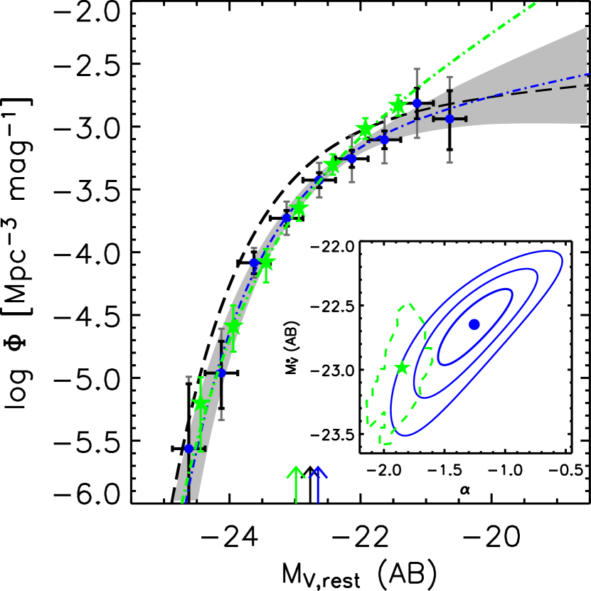
Figure 6.— Rest-frame $V$-band LF of blue galaxies at redshift $2.7\leq z\leq 3.3$ (blue dot-dashed line and filled circles) and $z\sim 3$ LBG LF (shapley01) (green dot-dashed and filled stars); the shaded area represents the 1 $\sigma$ uncertainties of the blue galaxy LF measured with the STY method; the global LF measured with the STY method is also plotted as a black long-dashed line; arrows represent the best-fit $M^{\star}$. The inset shows the best-fit value and the 1, 2, and 3 $\sigma$ confidence contour levels of the two parameters $\alpha$ and $M^{\star}$ for blue galaxies (blue filled circle and solid lines) and the 68.3% confidence intervals for the LBG best-fit Schechter parameters from (shapley01) (green filled star and dashed line).

4.4. Comparison with Previous Studies

In Appendix LABEL:app-3 we compare our results with previously published LFs. Specifically, we have compared our rest-frame $B$-band LF with that derived by poli03, giallongo05, and gabasch04 in the redshift intervals $2\leq z\leq 2.5$ and $2.5<z\leq 3.5$, and our rest-frame $R$-band LF with the rest-frame $r$-band LF derived by gabasch06 at $2\leq z\leq 2.5$. We also compared our rest-frame $B$-band LFs of red and blue galaxies at $2.5<z\leq 3.5$ with those measured by giallongo05.

5. Densities

5.1. Number Density and Field-to-Field Variance

The estimates of the number density $\eta$ obtained by integrating the best-fit Schechter function to the faintest observed rest-frame luminosity are listed in Table 4. For completeness, we also list $\eta^{\rm MUSYC}$, calculated by integrating the best-fit Schechter LF to the rest-frame magnitude limits of the NIR MUSYC, and $\eta^{+2}$, calculated by integrating the best-fit Schechter LF to 2 mag fainter than the faintest observed luminosities. We find that the contribution of DRGs (red galaxies) to the total number density down to the faintest probed rest-frame luminosities is 13%-25% (18%-29%) depending on the redshift interval. By integrating the rest-frame $B$-band LF down to a fixed rest-frame magnitude limit ($M_{\rm B,AB}=-20$), we find a hint of an increase of the contribution of blue galaxies from the low redshift bin (62%) to the higher bin (74%), but the differences are not significant. If only the bright end of the LF is considered (integrating the LF down to the fixed NIR MUSYC limit, $M_{\rm B,AB}=-22.2$), the increase of the contribution of the blue galaxy population becomes significant at the 2 $\sigma$ level, going from 42% in the low-$z$ bin to 66% in the high-$z$ bin.

Table 4Number Densities

			$\log{\eta}$	$\log{\eta^{\rm MUSYC}}$	$\log{\eta^{+2}}$
Redshift Range	Rest-Frame Band	Sample	(Mpc${}^{-3}$)	(Mpc${}^{-3}$)	(Mpc${}^{-3}$)
$2.0\leq z\leq 2.5$	$R$	All	$-2.61^{+0.07,0.11,0.16}_{-0.06,0.10,0.13}$	$-3.18^{+0.02,0.03,0.04}_{-0.02,0.03,0.04}$	$-2.36^{+0.17,0.29,0.42}_{-0.13,0.20,0.27}$
		$J-K>2.3$	$-3.48^{+0.07,0.14,0.21}_{-0.05,0.08,0.10}$	$-3.64^{+0.02,0.03,0.04}_{-0.02,0.03,0.04}$	$-3.48^{+0.09,0.19,0.31}_{-0.06,0.09,0.11}$
		$J-K\leq 2.3$	$-2.63^{+0.08,0.14,0.20}_{-0.08,0.13,0.17}$	$-3.37^{+0.02,0.03,0.04}_{-0.03,0.05,0.07}$	$-2.24^{+0.25,0.42,0.59}_{-0.18,0.29,0.39}$
		$U-V\geq 0.25$	$-3.19^{+0.07,0.12,0.17}_{-0.05,0.08,0.10}$	$-3.39^{+0.02,0.03,0.04}_{-0.02,0.03,0.04}$	$-3.18^{+0.09,0.17,0.28}_{-0.06,0.09,0.11}$
		$U-V<0.25$	$-2.72^{+0.10,0.16,0.22}_{-0.09,0.14,0.20}$	$-3.59^{+0.03,0.05,0.06}_{-0.04,0.08,0.11}$	$-2.25^{+0.31,0.52,0.73}_{-0.21,0.34,0.46}$
$2.7\leq z\leq 3.3$	$V$	All	$-2.51^{+0.07,0.11,0.16}_{-0.06,0.10,0.14}$	$-3.27^{+0.02,0.03,0.05}_{-0.03,0.05,0.07}$	$-2.16^{+0.19,0.33,0.47}_{-0.15,0.24,0.32}$
		$J-K>2.3$	$-3.17^{+0.12,0.21,0.30}_{-0.10,0.16,0.20}$	$-3.65^{+0.02,0.03,0.04}_{-0.03,0.06,0.10}$	$-3.05^{+0.26,0.50,0.76}_{-0.17,0.25,0.31}$
		$J-K\leq 2.3$	$-2.63^{+0.08,0.13,0.18}_{-0.07,0.12,0.16}$	$-3.49^{+0.03,0.05,0.06}_{-0.04,0.07,0.11}$	$-2.22^{+0.24,0.41,0.59}_{-0.19,0.30,0.40}$
		$U-V\geq 0.25$	$-3.25^{+0.11,0.20,0.28}_{-0.09,0.14,0.18}$	$-3.65^{+0.02,0.03,0.04}_{-0.03,0.05,0.08}$	$-3.19^{+0.21,0.40,0.64}_{-0.13,0.19,0.24}$
		$U-V<0.25$	$-2.61^{+0.08,0.13,0.18}_{-0.07,0.12,0.16}$	$-3.49^{+0.03,0.05,0.07}_{-0.04,0.07,0.11}$	$-2.17^{+0.24,0.41,0.59}_{-0.20,0.32,0.41}$
$2.0\leq z\leq 2.5$	$B$	All	$-2.53^{+0.08,0.13,0.19}_{-0.08,0.12,0.17}$	$-3.38^{+0.03,0.05,0.06}_{-0.03,0.06,0.09}$	$-2.15^{+0.25,0.42,0.60}_{-0.17,0.28,0.37}$
		$J-K>2.3$	$-3.34^{+0.17,0.30,0.42}_{-0.13,0.21,0.27}$	$-3.92^{+0.04,0.05,0.07}_{-0.05,0.11,0.17}$	$-3.19^{+0.42,0.80,1.23}_{-0.23,0.33,0.40}$
		$J-K\leq 2.3$	$-2.60^{+0.09,0.15,0.21}_{-0.08,0.14,0.19}$	$-3.53^{+0.04,0.06,0.07}_{-0.05,0.08,0.12}$	$-2.17^{+0.30,0.51,0.73}_{-0.20,0.33,0.43}$
		$U-V\geq 0.25$	$-3.07^{+0.13,0.23,0.33}_{-0.11,0.17,0.22}$	$-3.63^{+0.03,0.04,0.06}_{-0.04,0.08,0.12}$	$-2.95^{+0.29,0.58,0.88}_{-0.18,0.26,0.32}$
		$U-V<0.25$	$-2.71^{+0.10,0.16,0.23}_{-0.09,0.15,0.21}$	$-3.71^{+0.04,0.07,0.09}_{-0.06,0.10,0.16}$	$-2.23^{+0.35,0.59,0.83}_{-0.22,0.37,0.49}$
$2.5<z\leq 3.5$	$B$	All	$-2.43^{+0.07,0.12,0.17}_{-0.07,0.12,0.16}$	$-3.46^{+0.03,0.05,0.06}_{-0.04,0.06,0.09}$	$-1.92^{+0.23,0.39,0.54}_{-0.18,0.30,0.40}$
		$J-K>2.3$	$-3.04^{+0.15,0.26,0.36}_{-0.14,0.22,0.29}$	$-3.89^{+0.04,0.07,0.09}_{-0.06,0.12,0.19}$	$-2.68^{+0.42,0.76,1.10}_{-0.32,0.47,0.58}$
		$J-K\leq 2.3$	$-2.57^{+0.08,0.14,0.19}_{-0.08,0.13,0.18}$	$-3.65^{+0.04,0.06,0.08}_{-0.04,0.08,0.12}$	$-2.03^{+0.27,0.46,0.65}_{-0.22,0.35,0.47}$
		$U-V\geq 0.25$	$-3.06^{+0.16,0.27,0.38}_{-0.14,0.22,0.29}$	$-3.90^{+0.05,0.07,0.09}_{-0.07,0.12,0.20}$	$-2.74^{+0.44,0.78,1.14}_{-0.31,0.45,0.56}$
		$U-V<0.25$	$-2.56^{+0.08,0.14,0.19}_{-0.08,0.13,0.18}$	$-3.64^{+0.04,0.06,0.08}_{-0.04,0.08,0.12}$	$-2.00^{+0.26,0.45,0.64}_{-0.22,0.35,0.47}$

We determine the field-to-field variance in the density by fixing the parameters $\alpha$ and $M^{\star}$ to the best-fit values measured using the composite sample, and estimating $\Phi^{\star}_{\rm j}$ for each $j$th field separately by imposing a normalization on the LF such that the total number of observed galaxies in each field is reproduced. In Table 5, the derived $\Phi^{\star}_{\rm j}$ of DRGs and non-DRGs in each field are listed for the three targeted redshift intervals and compared to $\Phi^{\star}$ measured from the composite sample. The results in the redshift range $2.5<z\leq 3.5$ are plotted in Figure 7. We find an overdensity of DRGs in the M1030 field at all redshifts, with the excess (as compared to the characteristic density of the composite sample) varying from a factor of $\sim 1.2$ in the lowest redshift bin up to a factor of $\sim 1.9$ in the redshift interval $2.5<z\leq 3.5$. We also find an underdensity of DRGs (a factor of 0.82-0.86) in the GOODS-CDFS field, although only at $z>2.5$. The value of $\Phi^{\star}$ for DRGs in M1030 is a factor of $\sim 1.6$–2.4 larger than that in the GOODS-CDFS field at $z>2.5$, although they are similar at $2\leq z\leq 2.5$.

Table 5Characteristic Density $\Phi^{\star}$ in Each Field

Redshift Range	Composite Sample	MH2	MH1	M1030	CDFS	FMS	FH
DRGs
$2.0\leq z\leq 2.5$	$3.74^{+0.69}_{-1.09}$	$2.71^{+0.93}_{-0.73}$	$3.13^{+0.76}_{-0.62}$	$4.49^{+0.83}_{-0.71}$	$3.96^{+0.83}_{-0.70}$	$3.78^{+1.51}_{-1.12}$	$6.14^{+4.84}_{-2.93}$
$2.7\leq z\leq 3.3$	$6.14^{+1.10}_{-1.71}$	$7.41^{+2.26}_{-1.78}$	$6.45^{+1.43}_{-1.19}$	$8.49^{+1.46}_{-1.26}$	$5.25^{+0.94}_{-0.81}$	$2.70^{+1.23}_{-0.88}$	$7.79^{+3.84}_{-2.69}$
$2.5<z\leq 3.5$	$4.88^{+2.09}_{-2.20}$	$8.54^{+3.08}_{-2.33}$	$5.75^{+1.55}_{-1.24}$	$9.37^{+1.66}_{-1.42}$	$3.99^{+0.66}_{-0.57}$	$1.84^{+0.74}_{-0.55}$	$4.72^{+1.63}_{-1.25}$
non-DRGs
$2.0\leq z\leq 2.5$	$6.32^{+2.72}_{-2.41}$	$6.26^{+1.55}_{-1.27}$	$8.63^{+1.24}_{-1.09}$	$7.90^{+1.09}_{-0.96}$	$3.22^{+0.53}_{-0.46}$	$5.80^{+1.07}_{-0.91}$	$12.65^{+2.33}_{-1.99}$
$2.7\leq z\leq 3.3$	$11.14^{+4.02}_{-4.27}$	$11.49^{+3.80}_{-2.93}$	$13.44^{+2.44}_{-2.09}$	$13.52^{+2.17}_{-1.89}$	$9.65^{+1.14}_{-1.03}$	$6.70^{+1.46}_{-1.22}$	$18.68^{+3.35}_{-2.87}$
$2.5<z\leq 3.5$	$9.50^{+4.53}_{-3.92}$	$7.03^{+3.46}_{-2.43}$	$7.07^{+1.90}_{-1.53}$	$14.15^{+2.20}_{-1.92}$	$8.77^{+0.91}_{-0.83}$	$7.65^{+1.20}_{-1.05}$	$12.68^{+1.89}_{-1.66}$

Note. — Units in 10${}^{-4}$ Mpc${}^{-3}$ mag${}^{-1}$; the 1 $\sigma$ error of the characteristic density estimated for the individual field includes only the Poisson error (gehrels86). The measured rest-frame $R$-, $V$-, and $B$-band LFs have been used in the redshift ranges $2.0\leq z\leq 2.5$, $2.7\leq z\leq 3.3$, and $2.5<z\leq 3.5$, respectively.

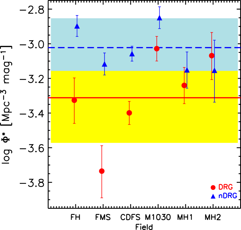
Figure 7.— Values of $\Phi^{\star}$ for DRGs (red filled circles) and non-DRGs (blue filled triangles) in the redshift range $2.5<z\leq 3.5$ estimated in the rest-frame $B$ band as described in § 5.1 for each individual field; the yellow (DRGs) and cyan (non-DRGs) shaded regions represent the values of $\Phi^{\star}$ from the analysis in § 3.2 on the composite sample.

These results are qualitatively consistent with vandokkum06, who showed that the GOODS-CDFS field is underdense in massive ($M_{\star}>10^{11}$ $M_{\sun}$) galaxies at $2<z<3$, with a surface density that is about 60% of the mean and a factor of 3 lower than that of their highest density field (M1030). However, our results seem to show systematically smaller underdensities for the GOODS-CDFS field compared to their work. In order to understand the origin of the smaller underdensity of DRGs found for the GOODS-CDFS field in our work compared to that of massive galaxies in vandokkum06, we have estimated the surface density of DRGs in the redshift range $2<z<3$ down to $K^{\rm tot}_{\rm s}=21$. We find that the surface density of DRGs in the GOODS-CDFS field is $\sim 70$% of the mean and a factor of $\sim 2.2\pm 0.5$ lower than that of the M1030 field, in good agreement with the values in vandokkum06. Therefore, the smaller underdensities of DRGs found for the GOODS-CDFS field in our work appear to arise mainly from the different targeted redshift ranges. The approach adopted in this work to quantify field-to-field variance by comparing the $\Phi^{\star}_{\rm j}$ of the individual fields might also mitigate field-to-field differences, especially at the bright end.

We note that there are significant differences in the observed characteristic densities even within the MUSYC fields, although they have areas of $\sim 100$ arcmin${}^{2}$. For example, the observed $\Phi^{\star}$ of DRGs in the MH1 field is consistent with the one derived from the composite sample, but it is 0.61-0.76 times the value in the M1030 field. These results demonstrate that densities inferred from individual $\sim 100$ arcmin${}^{2}$ fields should be treated with caution.

5.2. Luminosity Density

In this section we present estimates of the luminosity density. Because of the coupling between the two parameters $\alpha$ and $M^{\star}$, the luminosity density (obtained by integrating the LF over all magnitudes) is a robust way to characterize the contribution to the total LF from the different subpopulations and to characterize the evolution of the LF with redshift.

The luminosity density $\rho_{\rm L}$ is calculated using:

$$\rho_{\rm L}=\int^{\infty}_{0}{L_{\rm\nu}\Phi(L_{\rm\nu})dL_{\rm\nu}}=\Gamma(2+\alpha)\Phi^{\star}L^{\star},$$ (7)

which assumes that the Schechter parametrization of the observed LF is a good approximation and valid also at luminosities fainter than probed by our composite sample. Table 6 lists $\rho_{\rm L}$ with the corresponding 1, 2, and 3 $\sigma$ errors for all of the considered samples. We also list $\rho^{\rm last}_{\rm L}$, the luminosity density calculated to the faintest probed rest-frame luminosity, and $\rho^{\rm MUSYC}_{\rm L}$, the luminosity density calculated to the rest-frame magnitude limits of the deep NIR MUSYC. While the difference between $\rho_{\rm L}$ and $\rho^{\rm last}_{\rm L}$ is very small (negligible for DRGs and red galaxies, and $\sim 0.1$ dex on average for non-DRGs and blue galaxies), the difference between $\rho_{\rm L}$ and $\rho^{\rm MUSYC}_{\rm L}$ is significant, especially for non-DRGs and blue galaxies ($\sim 0.5$ dex on average).

Table 6Luminosity Densities

Redshift Range	Rest-Frame Band	Sample	$\log{\rho_{\rm L}}$	$\log{\rho^{\rm last\tablenotemark{a}}_{\rm L}}$	$\log{\rho^{\rm MUSYC\tablenotemark{b}}_{\rm L}}$
$2.0\leq z\leq 2.5$	$R$	All	$26.74^{+0.06,0.08,0.12}_{-0.05,0.06,0.07}$	$26.71^{+0.05,0.06,0.07}_{-0.05,0.06,0.07}$	$26.53^{+0.05,0.06,0.07}_{-0.05,0.06,0.07}$
		$J-K>2.3$	$26.18^{+0.05,0.06,0.08}_{-0.05,0.06,0.07}$	$26.18^{+0.05,0.06,0.08}_{-0.05,0.06,0.07}$	$26.14^{+0.05,0.07,0.09}_{-0.05,0.07,0.09}$
		$J-K\leq 2.3$	$26.64^{+0.10,0.20,0.43}_{-0.07,0.08,0.10}$	$26.57^{+0.05,0.06,0.07}_{-0.05,0.06,0.07}$	$26.30^{+0.06,0.08,0.10}_{-0.06,0.09,0.11}$
		$U-V\geq 0.25$	$26.43^{+0.05,0.06,0.07}_{-0.05,0.06,0.07}$	$26.43^{+0.05,0.06,0.07}_{-0.05,0.06,0.07}$	$26.37^{+0.05,0.06,0.07}_{-0.05,0.06,0.07}$
		$U-V<0.25$	$26.50^{+0.18,0.48,2.47}_{-0.09,0.12,0.14}$	$26.40^{+0.05,0.06,0.08}_{-0.05,0.06,0.07}$	$26.03^{+0.07,0.10,0.13}_{-0.08,0.12,0.16}$
$2.7\leq z\leq 3.3$	$V$	All	$26.97^{+0.08,0.15,0.26}_{-0.06,0.07,0.09}$	$26.91^{+0.05,0.06,0.07}_{-0.05,0.06,0.07}$	$26.61^{+0.05,0.07,0.08}_{-0.06,0.08,0.10}$
		$J-K>2.3$	$26.44^{+0.07,0.12,0.24}_{-0.05,0.06,0.07}$	$26.43^{+0.05,0.06,0.08}_{-0.05,0.06,0.07}$	$26.26^{+0.06,0.07,0.09}_{-0.06,0.09,0.13}$
		$J-K\leq 2.3$	$26.82^{+0.12,0.28,0.66}_{-0.07,0.10,0.12}$	$26.73^{+0.05,0.06,0.07}_{-0.05,0.06,0.07}$	$26.36^{+0.06,0.08,0.11}_{-0.07,0.10,0.13}$
		$U-V\geq 0.25$	$26.40^{+0.05,0.08,0.14}_{-0.05,0.06,0.07}$	$26.39^{+0.05,0.06,0.07}_{-0.05,0.06,0.07}$	$26.26^{+0.06,0.07,0.09}_{-0.06,0.08,0.12}$
		$U-V<0.25$	$26.84^{+0.13,0.31,0.85}_{-0.08,0.11,0.13}$	$26.74^{+0.05,0.06,0.07}_{-0.05,0.06,0.07}$	$26.36^{+0.06,0.08,0.10}_{-0.07,0.10,0.13}$
$2.0\leq z\leq 2.5$	$B$	All	$26.61^{+0.10,0.20,0.38}_{-0.07,0.09,0.11}$	$26.54^{+0.05,0.06,0.07}_{-0.05,0.06,0.07}$	$26.15^{+0.06,0.08,0.11}_{-0.06,0.09,0.13}$
		$J-K>2.3$	$25.90^{+0.10,0.27,2.95}_{-0.06,0.07,0.08}$	$25.89^{+0.06,0.09,0.13}_{-0.05,0.06,0.07}$	$25.64^{+0.08,0.11,0.15}_{-0.09,0.15,0.22}$
		$J-K\leq 2.3$	$26.53^{+0.15,0.35,1.15}_{-0.08,0.11,0.13}$	$26.43^{+0.05,0.07,0.08}_{-0.05,0.06,0.07}$	$25.99^{+0.07,0.10,0.13}_{-0.07,0.12,0.16}$
		$U-V\geq 0.25$	$26.18^{+0.07,0.14,0.31}_{-0.05,0.06,0.07}$	$26.17^{+0.05,0.07,0.10}_{-0.05,0.06,0.07}$	$25.92^{+0.06,0.08,0.11}_{-0.07,0.11,0.16}$
		$U-V<0.25$	$26.41^{+0.22,0.68,2.38}_{-0.10,0.14,0.16}$	$26.29^{+0.05,0.07,0.09}_{-0.05,0.06,0.07}$	$25.79^{+0.08,0.12,0.16}_{-0.09,0.14,0.21}$
$2.5<z\leq 3.5$	$B$	All	$26.90^{+0.16,0.37,1.00}_{-0.10,0.13,0.16}$	$26.75^{+0.05,0.06,0.08}_{-0.05,0.06,0.07}$	$26.28^{+0.06,0.08,0.09}_{-0.06,0.09,0.12}$
		$J-K>2.3$	$26.30^{+0.21,0.81,\infty}_{-0.10,0.13,0.14}$	$26.23^{+0.07,0.10,0.14}_{-0.06,0.07,0.09}$	$25.86^{+0.07,0.10,0.12}_{-0.09,0.15,0.22}$
		$J-K\leq 2.3$	$26.76^{+0.24,0.74,\infty}_{-0.12,0.16,0.19}$	$26.59^{+0.05,0.07,0.09}_{-0.05,0.06,0.07}$	$26.08^{+0.07,0.09,0.11}_{-0.07,0.11,0.15}$
		$U-V\geq 0.25$	$26.27^{+0.20,0.67,\infty}_{-0.09,0.12,0.13}$	$26.22^{+0.07,0.10,0.14}_{-0.06,0.07,0.09}$	$25.84^{+0.07,0.10,0.12}_{-0.09,0.15,0.23}$
		$U-V<0.25$	$26.79^{+0.25,0.93,\infty}_{-0.13,0.17,0.20}$	$26.60^{+0.05,0.07,0.09}_{-0.05,0.06,0.07}$	$26.09^{+0.07,0.09,0.11}_{-0.07,0.10,0.14}$

Note. — The luminosity densities are in units of erg s${}^{-1}$ Hz${}^{-1}$ Mpc${}^{-3}$. The quoted errors correspond to the 1, 2, and 3 $\sigma$ errors estimated from the maximum likelihood analysis as described in § 3.2 and include the contribution from photometric redshift uncertainties.