A sensitive submillimetre survey of Broad Absorption Line quasars

Abstract

Using the SCUBA bolometer array on the JCMT, we have carried out a submillimetre (submm) survey of Broad Absorption Line quasars (BALQs). The sample has been chosen to match, in redshift and optical luminosity, an existing benchmark 850$\mu$m sample of radio-quiet quasars, allowing a direct comparison of the submm properties of BAL quasars relative to the parent radio-quiet population. We reach a submm limit $1\sigma\approx$1.5mJy at 850$\mu$m, allowing a more rigorous measure of the submm properties of BAL quasars than previous studies. Our submm photometry complements extensive observations at other wavelengths, in particular X-rays with Chandra and infrared with Spitzer.

To compare the 850$\mu$m flux distribution of BALQs with that of the non-BAL quasar benchmark sample, we employ a suite of statistical methods, including survival analysis and a novel Bayesian derivation of the underlying flux distribution. Although there are no strong grounds for rejecting the null hypothesis that BALQs on the whole have the same submm properties as non-BAL quasars, we do find tentative evidence (1–4 percent significance from a K–S test and survival analysis) for a dependence of submm flux on the equivalent width of the characteristic C IV broad absorption line. If this effect is real— submm activity is linked to the absorption strength of the outflow— it has implications either for the evolution of AGN and their connection with star formation in their host galaxies, or for unification models of AGN.

1 INTRODUCTION

1.1 AGN feedback and Broad Absorption Line quasars

The extreme luminosity and relatively low space density of Active Galactic Nuclei (AGN) might be taken to imply that they constitute an unusual subset of all galaxies, and that the study of AGN gives us a lopsided view of cosmological processes. On the contrary, recent findings indicate that activity on the small scales surrounding the central supermassive black hole (SMBH) and its accretion disk may have a significant bearing on the AGN’s environment on galactic scales or even larger, playing an important role in the evolution of the host galaxy and the surrounding intergalactic medium. The ubiquity of SMBHs within galactic nuclei suggests that a phase of AGN activity is the rule rather than the exception. Furthermore, the discovery of a correlation between the mass of the SMBH and the velocity dispersion of stars in the bulge of the host (Ferrarese & Merritt, 2000; Gebhardt et al. 2000) hints that the evolution of each component— SMBH and stars— must, at some level, be linked.

Feedback from the AGN itself has been suggested as one mechanism by which the $M-\sigma$ relation could be established (Silk & Rees, 1998; Fabian, 1999; Granato et al. 2004), wherein outflows from an AGN-driven wind can unbind gas from the host galaxy, halting star formation and further black hole growth. The effect of AGN feedback (in the form of jets or of accretion disk winds) on the evolution of the host galaxy has also been posited as a solution to the mismatch between $\Lambda$CDM hierarchical galaxy formation models and observed galaxy luminosity functions (e.g. Benson et al. 2003). The study of the evolution of AGN, their host galaxies and their outflows, is therefore of great significance to cosmology and galaxy formation.

Evidence for outflows is found in about 15 percent (Reichard et al., 2003) of luminous, optically selected quasars, in the form of Broad Absorption Lines (BALs). BALs, characteristically in the C IV (1549Å) line, exhibit broad absorption troughs with high blueshifts, pointing to an origin in high velocity ($\sim$0.1c), radiation-driven outflows. Broadly speaking, three scenarios have been proposed to account for the BAL effect in quasars: (1) BALQs form a distinct class of AGN in their own right (disfavoured by the observed similarity between BALQ and non-BALQ optical/UV continua and emission lines: Weymann et al. 1991) (2) BAL winds are a generic feature of all AGN, but an orientation dependence restricts the visibility of lines to only $\sim$10–20 percent of the population (Weymann et al., 1991; Murray et al. 1995) (3) the BAL phenomenon represents a short-lived phase in the life-cycle of every AGN, during which the active nucleus is still enshrouded by gas and dust which covers a large fraction of the sky (Hazard et al. 1984; Voit, Weymann & Korista, 1993). Either of the latter two interpretations (characterised by Becker et al. 2000 as “unification by orientation” as opposed to “unification by time”) would have important implications for understanding the nature and evolution of AGN, and their relationship with their host galaxies.

1.2 Submillimetre observations of high-redshift quasars

Observations in the submillimetre (submm) band have opened an important window on the formation of massive galaxies (for a small cross-section of the work in this area, see e.g. Smail, Ivison & Blain 1997; Hughes et al. 1998; Scott et al. 2002; Borys et al. 2003; Mortier et al. 2005). Models of the coevolution of SMBHs and spheroids (e.g. Granato et al. 2004) predict that a substantial portion of the star formation within the hosts of luminous AGN ought to take place in a dust-enshrouded, submm-luminous mode; there could therefore be a direct link between the population of high-redshift submm galaxies and AGN. Deep Chandra X-ray observations of fields surveyed by the Submm Common-User Bolometer Array (SCUBA) indicate that AGN are present in a high fraction of submm galaxies, even when their bolometric luminosity is dominated by a starburst (Alexander et al. 2005), consistent with a SMBH gradually growing within a massive, star-forming galaxy. It could be, then, that submm galaxies and quasars represent similar populations observed at different points during their life cycle. Within this scenario, it has been speculated that BALQs— or some subclass of BALQs such as low ionization BAL quasars (LoBALs: BALQs that exhibit absorption in lines such as Mg II in addition to the usual C IV)— represent a youthful transitionary phase during which the AGN, initially embedded within a region of high star formation, expels its obscuring shroud of gas and dust (Voit, Weymann & Korista, 1993) and emerges to become a classical, optically selected quasar, as in the evolutionary scheme of Sanders et al. (1988).

To seek observational evidence of star formation-powered submm emission in high-redshift AGN, we and other groups have carried out a sequence of surveys of optically selected quasars at submm/mm wavelengths (e.g. radio-quiet quasars at $z\sim$2: Priddey et al. 2003a and Omont et al. 2003; at $z>4$: Carilli et al. 2001, Omont et al. 2001, Isaak et al. 2002; and $z>5$: Priddey et al. 2003b; Petric et al. 2003; Robson et al. 2004). A handful of BALQs were incidentally observed during these studies, exhibiting marginally higher detection rates compared with non-BAL quasars. In addition, a number of the most spectacular high-redshift submm sources were also known to be BALQs: for example, the lensed $z$=2.55 (low ionization) BAL quasar H1413+117 known as the “Cloverleaf” (Hughes et al. 1997 for submm data), or the luminous, lensed $z$=3.91 quasar APM08279+5255 (Lewis et al. 1998). The implied link between BALs and large submm luminosity (hence possibly star formation) could, if verified, provide support for the evolutionary, “unification by time” model, but the sample sizes were inadequate to confirm or refute this suggestion with statistical confidence.

Here we present a study of a sample of BAL quasars undertaken with the SCUBA submm bolometer array on the JCMT. As described below (Section 2.1), the sample has been selected to facilitate comparison with the benchmark sample of optically luminous, $z\sim 2$ quasars observed by Priddey et al. 2003a (hereafter P03). Explicitly, we wish to test the null hypothesis that the submm properties of BALQs and non-BAL quasars are identical (strictly, in this instance, that BALQs and non-BALs quasars have the same 850$\mu$m flux distribution). Ancillary goals of this work are: to determine accurately the typical submm properties of a well-selected, widely studied sample of BAL quasars, to establish the submm contribution to their broadband SEDs, and to search for dependence of submm flux on other observed properties.

2 SAMPLE SELECTION AND OBSERVATIONS

2.1 Sample selection & strategy

Our parent sample is derived from the catalogue of BALQs in the Large Bright Quasar Survey (LBQS: Hewett et al. 1995) identified by Weymann et al. (1991). This is a well suited sample for a number of reasons. The LBQS is a homogeneous, rigorously selected survey, and the BALQ subset has formed the target of several detailed, multiwavelength studies (e.g. optical: Weymann et al. 1991, X-ray (Chandra): Gallagher et al. 2006a; mid-infrared (Spitzer): Gallagher et al. 2006b). Also, the sample is well matched, in optical luminosity and redshift, to the SCUBA Bright Quasar Survey (SBQS) $z$=2 sample (P03). The LBQS was one of the sources for the $z$=2 SBQS; note that all the BALQs in our sample meet the SBQS selection criteria. (Indeed, some of them were incidentally observed during that project, but will be removed from the P03 sample for the purposes of defining a non-BAL quasar comparison sample.) The correspondence in ($z$,$M_{B}$) between the two samples is illustrated in Figure 1. Absolute $B$ band magnitudes ($M_{B}$) for the BALQs were extrapolated (assuming a spectral index $-$0.5) from measurements of the monochromatic continuum flux at rest wavelength $\approx$2000Å measured by Weymann et al. (1991). The definition of the original SCUBA (non-BAL) quasar surveys (optical luminosity criterion $M_{B}<-27.5$) (McMahon et al. 1999, Isaak et al. 2002) employed an Einstein–de Sitter cosmology with $\Omega_{\Lambda}$=0, $\Omega_{\rm M}$=1, $H_{0}$=50 km s^-1 Mpc^-1. However, in Figure 1 and Table 1, we have transformed $M_{B}$ into a flat cosmology with $\Omega_{\Lambda}$=0.73 and $H_{0}$=70 km s^-1 Mpc^-1 (Spergel et al. 2006), and the equivalent selection criterion is shown as the dotted curve. Over the redshift range $1.5<z<3$, the offset between the cosmologies is small (indeed, their distance moduli are equal at $z\approx 1.5$).

The majority of the targets are bona fide radio-quiet quasars, according to the definition of Stocke et al. (1992), who report 5GHz fluxes/upper limits for the majority of the sample. 1.4Ghz fluxes for the remainder were obtained from the FIRST (Faint Images of the Radio Sky at Twenty centimetres: White et al., 1997) and NVSS (NRAO VLA Sky Survey: Condon et al. 1998) catalogues. Only one object, LBQS B2211$-$1915 has a nearby (1.5 arcsec) radio source, with a 1.4GHz flux of 64mJy. However, this quasar was not detected at 850$\mu$m so its radio-loudness does not affect our analysis. For the remainder, the radio upper limits predict a negligible ($\la$0.1mJy) synchrotron component when extrapolated to the submm (e.g. using a spectral index of $-$0.7, as in McMahon et al. 1999).

The final selection of observed sources was determined by largely uncontrollable factors such as telescope scheduling, etc.

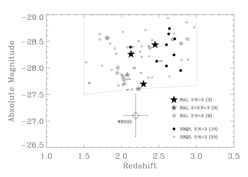
Figure 1: Selection criteria for the SCUBA BALQ sample. Star-shaped symbols indicate LBQS BALQs observed with SCUBA: $>$3$\sigma$ detections, 2$<\sigma<$3 tentative detections and $<$2$\sigma$ non-detections, as illustrated by the key (number of members of each class given in parentheses). For comparison, plotted as circles are quasars from the SBQS survey (Priddey et al. 2003a): $>$3$\sigma$ detections and non-detections (see key). The selection area is plotted as a dotted line. Finally, the large cross shows the mean $\pm$1$\sigma$ properties of the sample of Willott, Rawlings & Grimes (2003).

In previous SCUBA surveys of high-redshift quasars, we adopted a two-pronged strategy. For example in McMahon et al. (1999), a small $z>4$ sample was observed to a sensitive rms $\approx$1–1.5mJy in order to establish accurately the 850 and 450$\mu$m properties of high-redshift quasars. Isaak et al. (2002) and P03 (SBQS) pursued the complementary course of observing larger samples ($\approx$40 and 60 respectively) to a shallower limit, 1$\sigma\approx$3mJy, with the primary aim of sifting out the bright detections as targets for future follow-up. Since, however, the detection fraction at the limit of the SBQS was only $\sim$25 percent, the “typical” submm flux of the majority of $z$=2 quasars is clearly much fainter than this limit. The aims of the present BALQ programme (measure characteristic flux of BALQs, and precision photometry to constrain SEDs) thus require high sensitivity, and so an rms of 1.5mJy at 850$\mu$m was adopted. In parallel with, and complementary to, the survey of P03, a set of more sensitive data (1$\sigma\approx$1mJy) was also obtained for a small number (5) of (non-BAL) $z$=2 targets. Selection criteria, observing methods and data reduction were equivalent to those employed in P03 (q.v.). (For reference, we summarise the 850$\mu$m fluxes of these objects here: HS B0105+1619: 2.85$\pm$0.82mJy; HS B0218+3707: 0.95$\pm$1.17mJy; HS B0219+1452: 1.68$\pm$1.06mJy; HS B0248+3402: $-$0.49$\pm$1.08mJy; HS B2245+2531: 2.66$\pm$0.91mJy; though we defer any more detailed discussion of these objects to a separate paper (Priddey, Isaak & McMahon, in prep.).) These deeper data, in combination with the data from P03 minus known BALQs, we subsequently refer to as the “benchmark sample”.

2.2 Observations & data reduction

Observations were carried out at JCMT through the periods February–July 2003 and March–December 2004. Throughout the latter part of 2004, SCUBA experienced intermittent technical problems involving a 3-day warm-up cycle in the cryogen unit. A number of the observations reported in this paper were taken during this period, however the bulk of these data were obtained during a spell of stable behaviour. We have carefully inspected the affected observations nevertheless, to verify that the data appear to be of good quality.

The zenith opacity was monitored constantly via the JCMT Water Vapour Monitor (WVM), and regularly through skydips. These measurements were compared with each other and with the “Tau Meter” operated by the neighbouring Caltech Submm Observatory (CSO). Flux calibration was carried out, where possible, against the planets Uranus and Mars, and when planets were not visible, by using standard secondary flux calibrators.

Data reduction was performed using the automated ORAC-DR (Jenness et al., 2002) pipeline and, independently, using the SURF (Jenness & Lightfoot, 1998) package. Standard procedures were followed, involving: flatfielding, correction for atmospheric extinction, sky removal and clipping at the 3$\sigma$ level to remove spikes.

2.3 Comparison of strategy with other SCUBA BALQ surveys

An independent survey of the submm properties of BAL quasars (with similar scientific motivation) was carried out by Willott, Rawlings & Grimes (2003; hereafter WRG03). Their strategy was complementary to the one pursued here, aiming for a large (30 targets) sample observed to a relatively shallow (typically 2.5mJy rms) flux limit. They found no statistically significant difference between their BALQ sample, and the sample of P03. However, these two samples are not well matched, the SDSS-derived sample of WRG03 lying $\approx$2 magnitudes fainter in the optical than the sample of P03 (e.g. Figure 1). Thus, a comparison between their BALQ sample and the non-BAL quasars sample of P03 involves making additional, poorly constrained assumptions about the relation of submm with optical luminosity. Moreover, their larger observational uncertainty in principle precludes detailed study of the detected sources (for example accurate measurement of SEDs).

3 RESULTS AND ANALYSIS

850$\mu$m and 450$\mu$m fluxes for the sample are shown in Table 1. 15 BALQs were observed in total, for all but one of which (LBQS B2211$-$1915) our completeness criteria were met, i.e. an 850$\mu$m rms better than 1.5mJy or a detection better than 3$\sigma$. Note that only one of the observed sample, LBQS B1231+1320, is a known low-ionization BAL quasar (LoBAL); the others are all high-ionization BAL quasars (HiBALs). This is by happenstance rather than by design, the distinction between the classes not having formed part of our selection criteria. However, as LoBALQs make up $\sim$10 percent of optically selected BALQ samples, 1/15 is not unrepresentative.

Figure 2: Constraints on thermal dust SEDs for detected sources. The curves trace loci of the observed 450/850$\mu$m ratios (thick lines) and their $\pm$1$\sigma$ uncertainties (thin lines) or upper limit (thin dotted line for LBQS 0021$-$0213). For the 450$\mu$m-detected sources, either hot dust is required ($\sim$80K for a standard value for $\beta$ of 1.5), or a steep greybody spectral index $\beta\approx 2$ (consistent with $z>4$ quasar submm SEDs: Priddey & McMahon 2001). Inevitably, the relative insensitivity at shorter submm wavelengths biases us toward being able to measure temperatures preferentially for hotter sources.

3.1 Detected sources

Three BALQs are detected with $>$3$\sigma$ significance at 850$\mu$m (0019+0107, 0021$-$0213, 1443+0141). In addition, a further three targets are tentatively detected at the 2–3$\sigma$ level of significance. If we also include data from P03, then the total coadded 850$\mu$m flux density for one of these marginal sources, LBQS B0025$-$0151, becomes 3.8$\pm$1.2mJy— confirming its detection at $>$3$\sigma$ significance. Note, however, that its flux lies below the formal detection limit of the complete sample, 4.5mJy (3$\sigma$), so it will not be taken into account in, for example, the detection rate estimate (below).

Two sources are also detected at 450$\mu$m, with $>$3$\sigma$ significance (0019+0107 and 1443+0141). Although the 450$\mu$m rms errors are large (combined with which one must also take into account a calibration error of $\sim$20 percent, when converting from a signal in volts to a flux density in mJy), the 850/450$\mu$m flux ratios may be used to make crude estimates of the temperature of the emitting dust. Figure 2 shows the constraints placed on an isothermal dust SED parametrized by temperature and greybody index $\beta$. The two sources detected at 450$\mu$m require hot dust ($\ga$80K) if a typical value of 1.5 is assumed for $\beta$. However, for $\beta$=2, the temperatures descend to $\approx$40K— consistent with submm SEDs determined for $z>4$ quasars by Priddey & McMahon (2001). In contrast, a firm upper limit can be placed on the 450/850$\mu$m ratio of LBQS B0021$-$0213, placing a 2$\sigma$ upper limit on the dust temperature of $\la$40K.

Further multiwavelength data are needed to break the $T-\beta$ degeneracy, and thereby determine the origin of the submm emission. A low dust temperature would be suggestive of emission not from the central regions of the AGN, but from the kpc scales of the host galaxy, possibly from regions of massive star formation. Taking $T$=40K, $\beta$=2.0, the integrated thermal luminosity, in the far-infrared, of LBQS B0019+0107 is $L_{\rm FIR}$=1.6$\pm$0.5$\times$10¹³L_⊙, translating to an instantaneous rate of massive stars of $\sim$2000M_⊙ yr^-1 (e.g. following the same method and assumptions as in Isaak et al. (2002)). On the other hand, a hot temperature would be expected from dust in close proximity to the AGN, lying either in a “unified scheme” torus, or associated with the BAL wind. Taking $T$=80K, $\beta$=1.5, the far-infared luminosity of 0019+0107 is $L_{\rm FIR}$=1.3$\pm$0.4$\times$10¹⁴L_⊙— comparable with the bolometric luminosity $L_{\rm bol}\approx$2$\times$10¹⁴L_⊙ inferred from the optical (e.g. using the $B$ band bolometric correction factor of Elvis et al. 1994). Observations with the MIPS and IRAC instruments on Spitzer, which could shed light on the question of the location of the dust and the origin and energetics of the dust-heating light, have been obtained for all of the current sample, and these will be discussed in a forthcoming paper (Gallagher et al. 2006b).

Table 1: Submm fluxes of the LBQS BALQ sample. Statistically significant detections ($>3\sigma$) are shown in bold.

Source name	$z$	$B_{\rm J}$	$M_{B}$	$S_{850}$	$S_{450}$
				(mJy)	(mJy)
LBQS B0019+0107	2.130	18.09	$-$28.3	8.2$\pm$2.3	50$\pm$16
LBQS B0021$-$0213	2.293	18.68	$-$27.7	5.3$\pm$1.1	3.8$\pm$6.8
LBQS B0025$-$0151	2.076	18.06	$-$27.9	3.5$\pm$1.4	$-$2$\pm$16
+ additional data from Priddey et al. (2003)				3.8$\pm$1.2
LBQS B0029+0017	2.253	18.64	$-$27.6	5.2$\pm$2.0	19$\pm$11
LBQS B1029$-$0125	2.029	18.43	$-$27.7	1.0$\pm$1.2	4.4$\pm$6.4
LBQS B1208+1535	1.961	17.93	$-$27.9	2.2$\pm$1.4	16$\pm$9
LBQS B1231+1320	2.380	18.84	$-$28.4	$-$0.1$\pm$1.4	1.3$\pm$7.5
LBQS B1235+0857	2.898	18.17	$-$28.5	1.2$\pm$1.1	$-$7.5$\pm$6.9
LBQS B1235+1453	2.699	18.56	$-$28.5	1.9$\pm$1.4	$-$10$\pm$20
LBQS B1239+0955	2.013	18.38	$-$27.8	$-$0.7$\pm$1.0	$-$5.7$\pm$5.4
LBQS B1243+0121	2.796	18.50	$-$28.5	1.6$\pm$1.1	$-$4.6$\pm$7.2
LBQS B1443+0141	2.451	18.20	$-$28.4	5.2$\pm$1.2	33.8$\pm$8.5
LBQS B2154-2005	2.035	18.21	$-$27.8	2.2$\pm$1.5	10$\pm$11
LBQS B2201$-$1834	1.814	17.81	$-$28.6	3.0$\pm$1.5	$-$25$\pm$13
LBQS B2211$-$1915	1.952	18.02	$-$28.0	0.8$\pm$1.65	$-$19$\pm$19

3.2 Comparison with non-BAL quasars

Figure 1 illustrates the correspondence in selection criteria between the $z\sim 2$ sample from P03, and the final BALQ sample observed here.

Considering the SCUBA-observed BALQ sample, out of 14 targets observed down to the completeness limit ($\sigma$=1.5mJy), 3 are detected at $>$3$\sigma$ significance. This gives us a detection fraction of 0.21$\pm$0.12. If we set the detection threshold at $>$2$\sigma$, the fraction becomes 0.43$\pm$0.17. Using a fit to the flux density distribution of the benchmark sample (see below for details), a lognormal function with median flux 2.00mJy and standard deviation 0.38dex, we predict a 3$\sigma$ (2$\sigma$) detection fraction, for a survey attaining 1.5mJy rms, of 0.21 (0.42) (Table 4)— closely consistent with the observed detection fraction of BALQs (notwithstanding the large uncertainty in the latter). Thus from a simple detection rate analysis, it appears that our data confirm the finding of WRG03, that BALQs as a class are not significantly brighter in the submm than the general $z$=2 radio-quiet quasar population. In the next two sections we investigate more detailed methods of comparison.

3.3 Survival analysis

The statistical methods of survival analysis can be used to take into account information from upper limits— or “left censored data”. To examine the null hypothesis $\rm{H_{0}}$ that BALQs and non-BAL quasars have the same submm flux density distribution, we have carried out the tests described by Feigelson & Nelson (1985) (using the software package ASURV, La Valley et al. 1992), enabling intercomparison of two censored datasets. The tests return the significance level at which $\rm{H_{0}}$ may be rejected. Table 2 shows the results of comparing the BALQ samples against the benchmark sample. Mean fluxes obtained from the censored data using the Kaplan–Meier estimator, along with significance levels corresponding to the comparison with the benchmark sample, are also given. Two conventions for discriminating between detections and non-detections are employed: A. signal-to-noise$\geq$3$\longrightarrow$detection; B. signal-to-noise$\geq$2$\longrightarrow$detection. (Note that the latter convention is used by WRG03.) We employ a conservative estimate of the value of the upper limit, corresponding to $S_{\rm ul}$=max($S$,0)+2$\sigma$, rather than the alternative $S_{\rm ul}$=2$\sigma$.

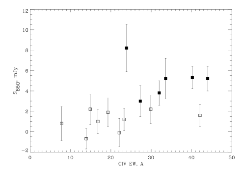
Figure 3: 850$\mu$m flux density plotted against equivalent width of the C IV broad absorption line. Submm detections ($>2\sigma$) are plotted as filled squares; non-detections as open squares (as points, at the value of their measured fluxes $\pm$1$\sigma$). It is apparent that large EWs ($\ga$25Å) dominate the detected sources: the K–S probability that the detections and non-detections have the same EW distribution is $\approx$0.01.

Table 2: Survival analysis of the three samples. The table is split according to whether a signal-to-noise ratio greater than 3 or 2 is taken to imply a detection (A and B respectively). $p$ is the probability of the null hypothesis that the samples have the same 850$\mu$m flux distribution. These tests are carried out between the BALQ samples and the benchmark $z$=2 sample (see text).

Sample:	benchmark	WRG03	LBQS	WRG03+LBQS
	$z$=2 non-BAL	faint BALQs	bright BALQs	all BALQs
A. Censored $\longleftrightarrow$ S:N $<$3
Mean	3.72$\pm$0.48	5.06$\pm$0.36	3.72$\pm$0.48	3.42$\pm$0.44
$p$ logrank	—	0.99	0.70	0.83
$p$ Gehan	—	0.93	0.48	0.77
$p$ Peto–Peto	—	0.97	0.62	0.83
$p$ Peto–Prentice	—	0.97	0.67	0.84
B. Censored $\longleftrightarrow$ S:N $<$2
Mean	4.52$\pm$0.47	5.11$\pm$0.35	4.52$\pm$0.47	3.15$\pm$0.62
$p$ logrank	—	0.96	0.21	0.30
$p$ Gehan	—	0.47	0.11	0.16
$p$ Peto–Peto	—	0.78	0.14	0.26
$p$ Peto–Prentice	—	0.74	0.16	0.24

Employing several estimators to perform the comparison (see Feigelson & Nelson 1985 for details), Table 2 shows that the null hypothesis, that BALQs and non-BAL quasars have identical submm flux distributions, cannot be rejected with any strong degree of confidence (i.e. at a significance level $p\la 0.05$). The largest disparity, according to this method, occurs between the SCUBA-observed LBQS BALQ sample and the benchmark sample, but since this is at best only $\approx$10 percent probable, the result is only marginal, and could be an artefact of the deeper limit reached in the LBQS sample.

We can also use bivariate survival analysis (Isobe, Feigelson & Nelson, 1986) to test for correlations between submm flux and other observables. Censoring at the 2$\sigma$ level, there appears to be a marginally significant correlation between submm flux and the equivalent width (EW) of the characteristic C IV broad absorption line ($p\equiv$probability that no correlation is present$\approx$0.04: Table 3). Figure 3 illustrates that six of the eight largest EWs correspond to submm detections; whilst below $\approx$25Å there are no detections at all. Indeed, the Kolmogorov–Smirnov (K–S) two-sample test returns a probability of 0.01 that the detections and non-detections have the same C IV EW distribution— a statistically significant result.

On the other hand, the Balnicity Index (BI: Weymann et al. 1991), a more conservative measure of the C IV EW (counting only high-velocity ($>$3000km s^-1) absorption above 2000 km s^-1 in width), returns a somewhat lower significance for the correlation test ($p\approx 0.09$: Table 3). Although the BI is well correlated with CIV EW for the LBQS BAL sample as a whole, the discrepancy could be explained by a large scatter in this correlation ($\sim$10 percent), which increases (to $\sim$25 percent) at low equivalent widths (below $\sim$25Å)— smearing out any effect such as that seen in Figure 3. Similarly, submm flux against the optical–X-ray spectral index $\alpha_{\rm ox}$, which is itself correlated with the C IV EW for low-redshift ($<$0.5) radio-quiet quasars (including a handful of BALQs) (Brandt, Laor & Wills, 2000), returns no hint of a correlation. For this reason, combined with its reliance upon a 2$\sigma$ detection threshold, we consider the $S_{850}$–C IV result extremely suggestive, but not, without further observation, conclusive.

Table 3: Tests for correlations between 850$\mu$m flux and other observables of the sample. $\alpha_{\rm uv}$ is the ultraviolet continuum slope, and $\Delta\alpha_{\rm ox}$ is a proxy for the amount of X-ray absorption (see Gallagher et al. 2006a). $p_{corr}$ is the probability that no correlation is present; $p_{KS}$ is the Kolmogorov–Smirnov probability that the detections and non-detections have the same distribution of the variable. (N.B. the Spearman’s Rho estimator has not been used because it is deemed to be unreliable for small datasets)

Variable	C IV EW	BI	$\alpha_{\rm uv}$	$\Delta\alpha_{\rm ox}$
	$p_{\rm corr}$
Proportional Hazard	0.037	0.082	0.35	0.22
Kendall’s Tau	0.041	0.095	0.50	0.11
	$p_{\rm KS}$
K–S two-sample	0.011	0.36	0.98	0.53

3.4 Flux density distribution— Bayesian method

It is noteworthy that the vast majority of the 850$\mu$m fluxes are positive (with a mean significantly different from zero), despite careful sky removal. In contrast, 450$\mu$m fluxes are both negative and positive, as one would expect for an average signal consistent with zero. This effect was scrutinized in detail in our previous submm photometric surveys, e.g. Isaak et al. (2002), where a careful comparison between on- and off-source bolometers revealed a net positive, on-source flux. A reasonable interpretation is that, at 850$\mu$m, we are measuring a real, non-zero flux distribution— a distribution with a positive characteristic flux density (e.g. the “fiducial” flux discussed by McMahon et al. 1999) and a width reflecting an intrinsic spread— which has been further smeared out by observational noise. This poses a problem, inter alia, as to what to do with fluxes lying at the 2–3$\sigma$ level: whether or not to consider them as “detections”, and how much confidence to attach to the measured signals. At low signal-to-noise, there is the risk of artificially boosting fluxes if the effects of Malmquist bias are not properly taken into account; on the other hand, setting too stringent a detection threshold discards potentially useful information about the underlying flux distribution.

To quantify these effects, and to estimate the range of true submm flux distributions that are consistent with our observations, we invert the problem via a Bayesian technique— starting from a range of models and iteratively updating the probability distributions over their parameters by comparison with each observed source. Details of this technique are described in Appendix A; in companion papers (e.g. Priddey, Isaak & McMahon, in prep.) we explore its application to a wider range of submm datasets than required for the current BALQ analysis.

Taking a lognormal distribution as an illustrative example, contours of the final probability distribution over its parameters— median ($S_{0}$) and standard deviation ($\Sigma_{10}$: in dex units, denoted by upper case $\Sigma$ to distinguish it from the rms submm flux density $\sigma$)— are shown in Fig 4. Also plotted is the marginal distribution for $S_{0}$ (calculated by integrating over the final joint probability distribution $P(S_{0};\Sigma_{10})$ with respect to $\Sigma_{10}$). $S_{0}$ provides a formal measure of the “fiducial flux” of McMahon et al. (1999), the characteristic flux density of the underlying distribution. For the LBQS BALQ sample, the most probable value for $S_{0}$=2.02mJy, and for $\Sigma$ it is 0.30dex. The best fit distribution is plotted as differential and cumulative histograms, together with the data. In these figures, the plotted model distribution does not directly represent the underlying distribution, but has been smoothed so as to represent the observed distribution that would be obtained if all observations had the same rms flux (equal in this case to the mean rms of the sample). Note, however, that the parameter estimation method is more subtle than this, taking full account of individual rms values (i.e. it is not as simple as deconvolving an observed histogram with a constant rms).

As noted above (Section 3.2), we can also apply the same analysis to the benchmark $z$=2 quasars and to the WRG03 samples (Table 4). Although the datasets employ complementary strategies (e.g. broad-but-shallow versus deep-but-narrow), the Bayesian method takes account of the differing rms values, making it possible to combine the two BALQ samples within a single analysis. Table 4 shows that the samples are, on the whole, consistent with each other, supporting the conclusions of the other statistical techniques we have used in this paper.

We have also applied the procedure to the 450$\mu$m fluxes of the current LBQS BALQ sample (the other samples do not have adequate 450$\mu$m data). In this case, the weighted mean is not significantly different from zero (though it is positive, as expected given the two statistically significant 450$\mu$m detections), and although fits are obtained, their quality is poorer than for the 850$\mu$m samples (N.B. only the Gaussian distribution allows for a negative characteristic flux, to act as a “sanity check” on the method in case of overall null detections: the other distributions assume that in the absence of noise, real astronomical objects have positive fluxes!).

Figure 4: Lognormal fit to the 850$\mu$m flux distribution of the LBQS BALQ sample. Top left, log likelihood contours over the lognormal parameters. The model with the highest likelihood is plotted with a star symbol, and contours correspond to (1,2,3,4)$\sigma$. Top right, marginal distribution over median flux (probability relative to peak). Models where $S_{0}\approx 2$mJy are strongly favoured. Bottom left, histogram of observed fluxes, with the underlying best-fit distribution plotted as a dotted curve. The dashed curve simulates the distribution that would actually be observed, given the best fit, assuming a constant rms is obtained (equal to the observed sample average in this case) Bottom right, as bottom left, but plotted as a cumulative histogram.

Table 4: Properties of the 850$\mu$m flux distributions of $z\sim 2$ BALQ and non-BAL quasar samples (and 450$\mu$m distribution of the LBQS BALQ sample: the others do not have adequate 450$\mu$m data). The first four rows are non-parametric statistical measures (average rms, then mean, median and variance-weighted flux density), the remainder describe the Bayesian estimates of the underlying distributions: lognormal, Schechter and Gaussian distributions (see Appendix A, Equations A1–A3 for functional forms). The BALQ sample from this paper is designated “LBQS”. $f_{\rm det}(>4.5)$ and ($>3.0$) are the predicted 3$\sigma$ (2$\sigma$) detection fractions assuming a (consistent) survey limit 1.5mJy.

Sample:	benchmark	WRG03	LBQS	WRG03 + LBQS	LBQS
	$z$=2 non-BAL	faint BALQs	bright BALQs	all BALQs	(450$\mu$m)
$<\sigma>$	2.67	2.53	1.40	2.15	10.9
$<S>$	2.89	2.56	2.70	2.62	4.3
$S_{med}$	2.33	3.45	2.20	2.20	1.3
$<S>_{w}$	2.53$\pm$0.29	2.55$\pm$0.45	2.28$\pm$0.34	2.41$\pm$0.27	3.2$\pm$2.2
lognormal $S_{0}$	2.00$\pm$0.50	2.02$\pm$0.65	2.02${}_{-0.60}^{+0.50}$	2.05$\pm$0.45	1.4${}_{-1.1}^{+2.6}$
$\Sigma_{10}$	0.38${}_{-0.07}^{+0.10}$	0.33${}_{-0.11}^{+0.15}$	0.30${}_{-0.10}^{+0.13}$	0.31${}^{+0.10}_{-0.07}$	0.85${}_{-0.3}^{+1.0}$
$f_{\rm det}(>4.5)$	0.21	0.20	0.18	0.19	—
$f_{\rm det}(>3.0)$	0.42	0.41	0.40	0.41	—
Schechter $S_{0}$	2.9$\pm$1.3	1.98${}^{+1.8}_{-1.0}$	1.26${}_{-0.6}^{+1.4}$	1.60${}_{-0.60}^{+1.0}$	15${}_{-7}^{+9}$
$\alpha$	0.0${}_{-0.3}^{+0.5}$	0.33${}_{-1.0}^{+1.5}$	1.00${}^{+2.0}_{-1.0}$	0.60${}_{-0.8}^{+1.0}$	$-$0.5${}_{-0.1}^{+0.3}$
$f_{\rm det}(>4.5)$	0.25	0.22	0.20	0.21	—
$f_{\rm det}(>3.0)$	0.45	0.43	0.42	0.43	—
Gaussian $S_{0}$	2.74$\pm 0.5$	2.53$\pm$0.6	2.49${}^{+0.6}_{-0.5}$	2.53$\pm$0.45	2.5$\pm$2.5
$\Sigma$	2.53±0.45	2.34$\pm$0.65	1.61${}^{+0.5}_{-0.4}$	1.94$\pm$0.45	3.3${}^{+1.7}_{-2.0}$
$f_{\rm det}(>4.5)$	0.32	0.28	0.20	0.24	—
$f_{\rm det}(>3.0)$	0.55	0.52	0.46	0.49	—

4 DISCUSSION

Both the geometry and the lifetime of BAL outflows are poorly constrained, to the extent that the observed fraction of BALQs amongst the general quasar population ($\sim$15 percent), could be accounted for either as an effect of orientation, of evolution, or of some combination of both. In the geometric interpretation, an anisotropic outflow, such as an accretion disk wind (e.g. Murray et al. 1995), is believed to be a feature of all AGN which is, however, only visible along a narrow range of sightlines. In this model, whether the observer sees a Type 1 (broad-line, unabsorbed) quasar, Type 2 (narrow-line, absorbed) quasar or BALQ (broad-line absorbed), depends on viewing angle. The contrasting evolutionary model holds that BALs occur when the AGN has been recently (re)fuelled, cocooned within a dense cloud of gas and dust, possibly coinciding with a major starburst. The BAL outflows may, furthermore, play a role in terminating further accretion and star formation, marking the transition between obscured AGN and classical, optical- and soft X-ray-luminous quasar.

Evidence for and against the evolutionary as opposed to the orientation model is, currently, somewhat mixed. Similar optical emission-line and continuum properties suggest that BALQs and non-BAL quasars belong to the same class (Weymann et al. 1991; Reichard et al. 2003), and results from spectropolarimetry favour an equatorial viewing plane for BALQs (Ogle et al. 1999). In contrast, radio spectral studies of both radio-loud (Becker et al. 2000) and radio-quiet (Barvainis & Lonsdale 1997) BALQs show that BALQs exhibit a mixture of radio spectral indices, both flat (core-dominated, pole-on) as well as steep (lobe-dominated, edge-on), indicating a range of observed lines of sight.

On which side of the fence do our results sit? At face value, the observed similarity between BALQs and non-BAL quasars in the submm would suggest that we are indeed observing intrinsically identical populations. This conclusion was favoured by WRG03, and our deeper limits and more rigorous selection would seem to lend it greater force. However, we have demonstrated (for example by our Bayesian derivation of the flux density distribution) that $z$=2 quasars, BAL and non-BAL alike, are typically very faint in the submm ($\sim$2–3mJy). The differences between BALQs and non-BAL quasars, if any, presumably lie further down the luminosity function than current (single aperture) submm surveys, with relatively bright confusion limits, can reach.

On the other hand, our tentative finding of a submm dependence on C IV EW (a large EW seems to be a necessary, but not sufficient, condition for submm detectability, since two high EW BALQs are nevertheless not detected: Figure 3) suggests that yet more rigorous selection criteria would yield substantially higher submm detection rates compared with non-BAL quasars.

It is of course possible that this effect results from selection biases, for example due to reddening. The most reddened quasars must be intrinsically more luminous to meet the $B_{J}$ selection criterion of the LBQS. If the C IV EW were, for whatever reason, correlated with reddening, this bias could induce the apparent correlation with submm flux. Nevertheless, assuming that our sample is homogeneous in terms of intrinsic luminosity, and that our submm–C IV EW relation is valid, what are its implications?

It is well known that BALQs are weaker in X-rays, relative to the optical, than non-BAL quasars— an effect believed to be due to absorption rather than an unusual intrinsic spectrum (e.g. Green et al. 1995; Gallagher et al. 2006a). Indeed, Brandt, Laor & Wills (2000) discovered, for a sample of low-redshift ($z<0.5$) quasars, a correlation between their C IV EW and soft X-ray weakness as measured by the optical–X-ray continuum (2500Å–2 keV) spectral index ($\alpha_{\rm ox}$). This connection between UV and X-ray absorption does not hold so straightforwardly for $z\sim 2$ LBQS quasars (Gallagher et al. 2006: Fig. 6a). Nevertheless, if our $S_{850}$–C IV EW connection is real, it could loosely be interpreted to advocate a link between submm activity, UV absorption and X-ray absorption. The link need not be direct, however, since the components responsible for each effect are likely to be distinct (this could account for the findings of Gallagher et al. 2006a). For example, X-ray absorption is an important feature of radiation-driven wind models, in which a “shielding gas” component is proposed, without which the outflow would become overionized by soft X-rays, and UV resonance-line-driven radiation pressure would become ineffective. The submm-emitting region, in contrast, is likely to be much more extended, lying within for example a dust torus or the host galaxy.

A possible analogy could be drawn with Narrow Line Seyfert 1 (NLS1) galaxies. AGN of this class are believed to result from SMBHs with an accretion rate that is a high fraction of the maximal Eddington-limited rate, and high velocity outflows have been observed in some (e.g. Pounds et al. 2003). It is possible that every young AGN— either freshly formed or recently refuelled following a merger— passes through such a high-Eddington state, launching an outflow, when gas supply to the nucleus is plentiful. Accompanying star formation could also result from, or play an active role in (e.g. Thompson, Quataert & Murray, 2005), the processes that drive gas into the nucleus. As the AGN luminosity increases as the SMBH grows, radiation pressure can generate BAL outflows of sufficient magnitude to terminate both star formation and further SMBH accretion.

Page et al. (e.g. 2004) found a similar submm dependence on X-ray absorption for a sample of $z\sim$2 quasars. In contrast with the canonical geometric unified schemes for AGN (e.g. Antonucci 1993), this is interpreted as evidence of an evolutionary sequence, rather like the schemes outlined above, between an initial, obscured, AGN–starburst phase, and a final unobscured phase, in which star formation has ceased. A BAL wind could act as the transitionary mechanism between these two phases.

An emerging point of view is that it is in fact the low-ionization BALQs that form a class distinct from other quasars (and from the more common HiBALs), perhaps a manifestation of youthful AGN, with a high covering factor of absorbing gas and perhaps dust (Boroson & Meyers, 1992; Voit, Weymann & Korista, 1993), and, indeed, the optical continua of LoBALs seem redder than those of other classes (Sprayberry & Foltz 1992; Reichard et al. 2003). One might expect a high detection fraction in the submm and infrared if that were the case, particularly if this youthful phase were accompanied by a starburst. The distinction between low- and high-ionization BALQs did not form part of our selection criteria. The single (known) LoBAL in our sample, LBQS B1231+1320, was not detected ($S_{850}$=$-$0.1$\pm$1.4mJy). However, it would still be of interest to obtain submm/mm observations of a sample of LoBALs, or the third, rarer subclass known as FeLoBALs (e.g. Becker et al. 1997).

In contrast to a starburst power source for the dust, the submm component could derive from optical/UV AGN emission reprocessed by nuclear dust. In this case, (i) larger C IV EW may merely be indicative of an intrinsically more luminous central engine. In support of this idea, Brandt, Laor & Wills (2000) found tentative evidence for a correlation between absolute visual magnitude ($M_{V}$) and C IV EW, though SCUBA and MAMBO samples (Omont et al. 2001; Isaak et al. 2002; Priddey et al. 2003; Omont et al. 2003) do not show, over the limited range of optical luminosities investigated in the present BALQ sample, such a strong correlation between optical and submm. Alternatively, (ii) if all AGN exhibited a distribution of wind covering fractions, then those that fill a larger solid angle of the sky would be more likely both to show high far-infrared luminosity (dust in the wind reprocesses a larger fraction of the AGN’s UV/optical output) and to exhibit BAL outflows (since a greater proportion of lines of sight intersect the wind).

Comparison of the submm fluxes and limits with the full SEDs (particularly X-ray and mid-infrared) will help constrain such speculation by casting light on the starburst versus AGN origin of the submm emission. But in either case, the implication of a dependence of submm flux on the properties of UV absorption lines provides support for the idea that the BAL phenomenon is not a simple geometric effect arising from a wind with a fixed covering fraction: since the X-ray- and UV-absorbing components are optically thin to submm radiation, the submm properties would not, all other factors being equal, be expected to depend on the observer’s viewing angle relative to the wind. It is, of course, quite possible that a non-trivial combination of variables (a range of lifetimes, covering factors and intrinsic luminosities) must be invoked to unify the BALQ class within the diverse ensemble of AGN types.

5 SUMMARY & CONCLUSIONS

We have observed a sample of $z$=2, optically luminous Broad Absorption Line quasars at submm wavelengths, using the SCUBA bolometer camera on the JCMT. Our goals were twofold:

(i) to test the null hypothesis $\rm{H_{0}}$: BALQs and non-BAL quasars have identical submm properties

(ii) to determine the 850$\mu$m flux distribution, the submm (850 + 450$\mu$m) contribution to the SEDs, and the relation between submm and other properties, of a well-selected, well-studied sample of BALQs.

The sample was selected so as to match, in redshift and optical luminosity, the “benchmark” submm sample of optically luminous, radio-quiet quasars observed by Priddey et al. (2003a) (supplemented with a small amount of additional data presented here). A direct comparison between BALQ and non-BAL quasars is thus possible. We have carried out this comparison in a number of different ways: 1. Simple non-parametric statistics such as means and medians; 2. Survival analysis; 3. A Bayesian method to disentangle the underlying flux distribution (once a suitable functional form is assumed) from the observed distribution. All these methods indicate that the submm properties of the BAL and non-BAL samples appear to be similar: $\rm{H_{0}}$ cannot be rejected with confidence. This conclusion is true for the luminosity-matched LBQS sample presented in this paper, as well as for the combined LBQS sample and that of WRG03 which, overall, spans a much larger range in optical luminosity. Note, however, that the LBQS sample generally shows larger deviations from the benchmark than the sample of WRG03 (though at best this effect is present at the $\sim$10 percent level). There is, moreover, some indication that optically fainter, non-BAL quasars at $z\sim$2 are also fainter in the submm (Priddey, Isaak & McMahon, in prep.). A comparison between the WRG03 sample and the optically faint $z$=2 sample would tentatively indicate that BALQs were systematically brighter in the submm than non-BAL quasars, but detailed characterisation and intercomparison of these two samples is limited by their large number of high rms, low-significance measurements.

The “typical” 850$\mu$m flux density of an optically luminous, $z$=2 BALQ is $\approx$2–3mJy (estimated by non-parametric methods and via the Bayesian fit to the flux distribution). Thus only with very deep submm/mm observations will it be possible to detect the majority of the BALQ population (when the difficulty will be encountering the confusion limit of current-generation, single-dish submm telescopes), and to carry out fully indicative tests of their submm properties relative to the general quasar population.

Some 450$\mu$m detections/upper limits enable crude estimates of the dust temperature. For a fuller discussion of the broadband SEDs (X-ray, optical, mid-infrared) of the LBQS BALQ sample, see Gallagher et al. (2006a) and Gallagher et al. (2006b). In principle, observations with Spitzer could discriminate spectrally between nuclear (e.g. AGN torus) and extended (e.g. star formation in host) dust components (for example by fitting template SEDs appropriate for each component).

Finally, we find tentative evidence for a dependence of submm flux on the equivalent width of the C IV broad absorption line. Although difficult to establish definitively with the present data, this finding would be easy to test by carrying out mm/submm observations of samples selected according to the EW criterion (specifically it would predict a high detection rate above EWs of $\approx$25Å). If this finding is correct— and whether the dust is heated by starburst or AGN— it suggests that the BAL phenomenon is not a simple geometric effect arising from an orientation-dependence on a wind with a fixed covering fraction, but that other variables, such as evolutionary phase, absorber covering fraction or intrinsic luminosity, must be invoked in order to unify BALQs with other classes of AGN.

Appendix A Bayesian estimation of the submillimetre flux density distribution

The so-called Bayesian interpretation of probability (that probabilities are a subjective measure of the plausibility of uncertain states of affairs) contrasts with the traditional, Frequentist interpretation (probabilities describe the relative frequencies of the outcomes of particular experiments). By adopting this point of view, and by using Bayes’ Theorem of conditional probabilities, one can develop a powerful method of deductive reasoning that tempers the idealised binary (“true” vs. “false”) certainty of classical logic, to a formalism that is better adapted to cope with the uncertainties inherent in scientific experimentation: a form of “quantitative epistemology” (Loredo, 1990). Bayesian techniques and philosophies are rapidly gaining ground in many areas of astrophysics. The interested reader is referred to the numerous reviews of the subject: see, in particular, Loredo (1990, 1992), or an introductory statistical text such as Wall & Jenkins (2003).

First, we must assume a functional form for the underlying submm flux distribution. In this paper, we have investigated three common functions, each characterised by a single pair of parameters, a characteristic flux $S_{0}$ and a width or a slope ($\Sigma$, $\Sigma_{10}$ or $\alpha$): (i) a lognormal distribution

$$n(S)\propto S^{-1}exp(-(\log{S}-\log{S_{0}})^{2}/2\Sigma_{10}^{2}),$$ (1)

(ii) the Schechter function (Schechter, 1976)

$$n(S)\propto\left(\frac{S}{S_{0}}\right)^{\alpha}exp(-S/S_{0}),$$ (2)

and (iii) the Normal (Gaussian) distribution

$$n(S)\propto exp(-(S-S_{0})^{2}/2\Sigma^{2}),$$ (3)

(The Gaussian distribution is unphysical in the sense that it attributes negative luminosities to submm sources. We include it here as a diagnostic of the method.) All are normalised so to give the correct total number of observed sources.

Our objective is to estimate the probability distribution— our subjective knowledge— over the parameter pairs ($S_{0}$; $\Sigma$, $\Sigma_{10}$, $\alpha$), by deriving the observational outcomes of each distribution and comparing with each data point in turn. The Bayesian method provides a way of updating this knowledge in the light of new data. First, for each function separately, we have to adopt a prior probability distribution over the parameters— call this $P(M_{j})$, where each model $M$ (described by pairs of ($S_{0}$; $\alpha$, $\Sigma$ or $\Sigma_{10}$) is denoted by the index j. In this paper, we have adopted uniform prior probability distributions, but in general one is free to take into account information from other sources in constructing the prior. Next (again, separately for each functional form) we iteratively update the probabilities in the light of each successive data point denoted by index i (having flux density $S_{i}$ and rms $\sigma_{i}$) by applying Bayes’ theorem:

$$P(M_{j}|S_{i},\sigma_{i})=P(M_{j})\times\frac{P(S_{i}|M_{j},\sigma_{i})}{\Sigma_{k}P(S_{i},\sigma_{i}|M_{k})}$$ (4)

where $P(S_{i}|M_{j},\sigma_{i})$ is the probability that, assuming model $M_{j}$ to be true, we would have measured a flux $S_{i}$ for the $i$th target— in this case, given by a convolution of the underlying flux distribution (given by $M_{j}$) with the error distribution describing the scatter of each data point (assumed to be Gaussian, with rms $\sigma_{i}$). The denominator acts as a normalising factor. $P(M_{j}|S_{i},\sigma_{i})$ now replaces $P(M_{j})$ as our estimate of the probability function over the parameters. We iterate the procedure with the next data point, using this new estimate of $P(M_{j})$ on the right hand side, and repeat until all data points have been taken into account. Note that for this purpose, all data are taken at face value, regardless of significance: their measurement error is taken into account in estimating $P(S_{i}|M_{j},\sigma_{i})$, alleviating the need to draw a sharp distinction between detection and non-detection.

If we are interested in the value of one parameter in particular— such as the characteristic flux, $S_{0}$— we can use the technique of Bayesian marginalization to integrate the final joint probability distribution ($P(S_{0};\alpha,\Sigma_{10},\Sigma)$) with respect to the remaining parameters (dubbed “nuisance parameters” in Bayesian analysis). The resulting marginal distribution ($P(S_{0})$) is the probability density function describing our subjective knowledge concerning the true value of the parameter ($S_{0}$). (N.B., this marginal distribution— e.g. top right panel of Figure 4— should not be confused with the “best guess” flux distribution (e.g. bottom panels of Figure 4) obtained by inserting the most likely values of the parameters into the function. The former is a measure of our subjective knowledge (or ignorance), the latter our best estimate of the real, objective distribution exhibited by the sample.)

The strength of the Bayesian approach is that we can take into account all the data, without making any distinction between “detection” and “non-detection”. This is particularly useful for treating low signal-to-noise data, for combining datasets which have a wide range of errors, or non-Gaussian errors, or which suffer from different observational biases (such bias could in principle be taken into account in estimating $P(S_{i}|M_{j},\sigma_{i})$ for each data point). Its weakness is its reliance upon our making an assumption about the functional form of the underlying distribution (The final $P(M)$ is, strictly, a conditional probability, the probability of the parameters taking particular values assuming the underlying form of the distribution to be true). This assumption may, in general, be motivated by a particular physical model, if independent evidence makes the model a priori more likely. For the present purposes, it is sufficient that the fit provide an adequate phenomological description of the data, in order that the key quantities can be estimated.

References

- Alexander (2005) Alexander D.M., Bauer F.E., Chapman S.C., Smail I., Blain A.W., Brandt W.N., Ivison R.J., 2005, ApJ, 632, 736
- Antonucci (1993) Antonucci R., 1993, ARA&A, 31, 473
- Barvainis & Lonsdale (1997) Barvainis R. & Lonsdale C., 1997, AJ, 113, 144
- Becker (1997) Becker R.H., Gregg M.D., Hook I.M., McMahon R.G., White R.L., Helfand D.J., 1997, ApJ, 479, L93
- Becker (2000) Becker R.H., White R.L., Gregg M.D., Brotherton M.S., Laurent-Muehleisen S.A., Arav N., 2000, ApJ, 538, 72
- Benson (2004) Benson A.J., Bower R.G., Frenk C.S., Lacey C.G., Baugh C.M., Cole S., 2003, ApJ, 599, 38
- Boroson & Meyers (1992) Boroson T.A. & Meyers K.A., 1992, ApJ, 397, 442
- Borys (2003) Borys C., Chapman S., Halpern M., Scott D., 2003, MNRAS, 344, 385
- Brandt, Laor & Wills (2000) Brandt W.N., Laor A., Wills B.J., 2000, ApJ, 528, 637
- Carilli (2001) Carilli C.L., et al., 2001, ApJ, 555, 625
- Condon (1998) Condon J.J., Cotton W.D., Greisen E.W., Yin Q.F., Perley R.A., Taylor G.B., Broderick J.J., 1998, AJ, 115, 1693
- Elvis (1994) Elvis M., et al., 1994, ApJS, 95, 1
- Fabian (1999) Fabian A.C., 1999, MNRAS, 308, L39
- Feigelson & Nelson (1985) Feigelson E.D., & Nelson P.I., 1985, ApJ, 293, 192
- Ferrarese & Merritt (2000) Ferrarese L., & Merritt D., 2000, ApJ, 539, L9
- Gebhardt (2000) Gebhardt K., et al., 2000, ApJ, 543, L5
- Gallagher (2006a) Gallagher S.C., Brandt W.N., Chartas G., Priddey R., Garmire G.P., Sambruna R.M., 2006, ApJ, 644, 709
- Gallagher (2006b) Gallagher S.C., Hines D.C., Blaylock M., Priddey R., Brandt W.N., Egami E.E., 2006, ApJ, submitted
- Granato (2004) Granato G.L., De Zotti G., Silva L., Bressan A., Danese L., 2004, ApJ, 600, 580
- Green (1995) Green P.J., et al., 1995, ApJ, 450, 51
- Hazard et al. (1984) Hazard C., Morton D.C., Terlevich R., McMahon R., 1984, ApJ, 282, 33
- Hewett (1995) Hewett P.C., Foltz C.B., Chaffee F.H., 1995, AJ, 109, 1498
- Hughes, Dunlop & Rawlings (1997) Hughes D.H., Dunlop J.S. & Rawlings S., 1997, MNRAS, 289, 766
- Hughes (1998) Hughes D., et al., 1998, Nature, 394, 241
- Isaak (2002) Isaak K.G., Priddey R.S., McMahon R.G., Omont A., Péroux C., Sharp R.G., Withington S., 2002, MNRAS, 329, 149
- Isobe, Feigelson & Nelson (1986) Isobe T., Feigelson E.D., & Nelson P.I., 1986, ApJ, 306, 490
- Jenness & Lightfoot (1998) Jenness T., Lightfoot J.F., Astronomical Data Analysis Software and Systems VII, A.S.P. Conference Series, Vol. 145, 1998, R. Albrecht, R.N. Hook and H.A. Bushouse, eds., p.216
- Jenness (2002) Jenness T., Stevens J.A., Archibald E.N., Economou F., Jessop N.E., Robson E.I., 2002, MNRAS, 336, 14
- La Valley (1992) La Valley M., Isobe T. & Feigelson E., 1992, in ASP Conference Series 25: Astronomical Data Analysis Software & Systems I, eds. D.M. Worrall, C. Biemesderfer & J. Barnes, vol. 1, 245
- Lewis (1998) Lewis G.F., Chapman S.C., Ibata R.A., Irwin M.J., Totten E.J., 1998, ApJ, 505, L1
- Loredo (1990) Loredo T.J., 1990, in Maximum Entropy and Bayesian Methods, P.F. Fougère (ed.), Kluwer Academic Publishers, Dordrecht, The Netherlands, 81
- Loredo (1992) Loredo T.J., 1992, in Statistical Challenges in Modern Astronomy, E.D. Feigelson & G.J. Babu (eds.), Springer-Verlag, New York, 275
- McMahon (1999) McMahon R.G., Priddey R.S., Omont A., Snellen I., Withington S., 1999, MNRAS, 309, L1
- Mortier (2005) Mortier A.M.J., et al., 2005, MNRAS, 363, 563
- Murray (1995) Murray N., Chiang J., Grossman S.A., Voit G.M., 1995, ApJ, 451, 498
- Ogle (1999) Ogle P.M., Cohen M.H., Miller J.S., Tran H.D., Goodrich R.W., Martel A.R., 1999, ApJS, 125, 1
- Omont (2001) Omont A., Cox P., Bertoldi F., McMahon R.G., Carilli C.L., Isaak K.G., 2001, A&A, 372, 371
- Omont (2003) Omont A., Beelen A., Bertoldi F., Cox P., Carilli C.L., Priddey R.S., McMahon R.G., Isaak K.G., 2003, A&A, 398, 857
- Page (2004) Page M.J., Stevens J.A., Ivison R.J., Carrera F.J., 2004, ApJ, 611, L85
- Petric (2003) Petric A.O., Carilli C.L., Bertoldi F., Fan X., Cox P., Strauss M., Omont A., Schneider D.P., 2003, AJ, 126, 15
- Pounds (2003) Pounds K.A., Reeves J.N., King A.R., Page K.L., O’Brien P.T., Turner M.J.L., 2003, MNRAS, 345, 705
- Priddey & McMahon (2001) Priddey R.S., & McMahon R.G, 2001, MNRAS, 324, L17
- Priddey (2003a) Priddey R.S., Isaak K.G., McMahon R.G., Omont A., 2003a, MNRAS, 339, L1183 (P03)
- Priddey (2003b) Priddey R.S., Isaak K.G., McMahon R.G., Robson E.I., Pearson C.P., 2003b, MNRAS, 344, L74
- Reichard (2003) Reichard T.A., et al., 2003, AJ, 126, 2594
- Robson (2004) Robson I., Priddey R.S., Isaak K.G., McMahon R.G., 2004, MNRAS, 351, L29
- Sanders (1988) Sanders D.B., Soifer B.T., Elias J.H., Neugebauer G., Matthews K., 1988, ApJ, 328, L35
- Schechter (1976) Schechter P., 1976, ApJ, 203, 197
- Scott (2002) Scott S.E., et al., 2002, MNRAS, 331, 817
- Silk & Rees (1998) Silk J., & Rees M.J., 1998, A&A, 331, L1
- Smail, Ivison & Blain (1997) Smail I., Ivison R.J., Blain A.W., 1997, ApJ, 490, L5
- Spergel (2006) Spergel D.N., et al., 2006, astro-ph/0603449
- Sprayberry & Foltz (1992) Sprayberry D. & Foltz C.B., 1992, ApJ, 390, 39
- Stocker (1992) Stocke J.T., Morris S.L., Weymann R.J., Foltz C.B., 1992, ApJ, 396, 487
- Thompson, Quataert & Murray (2005) Thompson T.A., Quataert E. & Murray N., 2005, ApJ, 630, 167
- Trump (2006) Trump J.R., et al., 2006, ApJS, 165, 1
- Voit, Weymann & Korista (1993) Voit G.M., Weymann R.J. & Korista K.T., 1993, ApJ, 413, 95
- Wall & Jenkins (2003) Wall J.V. & Jenkins C.R., Practical Statistics for Astronomers, 2003, Cambridge University Press
- Weymann (1991) Weymann R.J., Morris S.L., Foltz C.B., Hewett P.C., 1991, ApJ, 373, 23
- White (1997) White R.L., Becker R.H., Helfand D.J., Gregg M.D., 1997, ApJ, 475, 479
- Willott, Rawlings & Grimes (2003) Willott C., Rawlings S., Grimes J., 2003, ApJ, 598, 909