Helium and Iron in X-ray galaxy clusters

1 The metals in X-ray galaxy clusters

The X-ray emitting hot plasma in galaxy clusters represents the 80 per cent of the total amount of cluster baryons. It is composed by a primordial component polluted from the outputs of the star formation activity taking place in galaxies, that are the cold phase accounting for about 10 per cent of the cluster barionic budget (see Fig. 1).

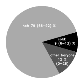
Figure 1: (Left) Updated version of the cluster baryonic pie presented in e03 and obtained by using $f_{\rm bar,WMAP}=0.176\pm 0.015$ from the best-fit results of the WMAP 3-yrs data (sp06 ), a depletion parameter $Y=0.920\pm 0.023$ and the gas and stellar mass fractions shown on the right which refer to a sample of 58 clusters with $T_{\rm gas}>4$ keV, redshift in the range $0.14-1.26$ and discussed in Ettori et al. (2006, in prep.). The dashed lines indicates the median value of $f_{\rm star}=0.016$ and $f_{\rm star}/f_{\rm gas}=0.129$.

As reference, a number density of $9.77\times 10^{-2}$ ions of helium and $4.68\times 10^{-5}$ ions of iron is expected for each atom of hydrogen in a hot plasma with solar abundance (as in ag89 ; for the most recent estimates in gs98 and a05 , the number density relative to H is $8.51\times 10^{-2}$ for He, $3.16\times 10^{-5}$ and $2.82\times 10^{-5}$ for Fe, respectively; see Table 1). These values imply a mass fraction of $(0.707,0.738)$ for H, $(0.274,0.250)$ for He and $(0.019,0.012)$ for heavier elements, accordingly to (ag89 , a05 ), respectively.

I discuss here some speculations, and relevant implications, of the sedimentation of helium in cluster cores (Sect. 2; details are presented in ef06 ) and a history of the metal accumulation in the ICM, with new calculations (with respect to the original work in e05 ) following the recent evidence of a bi-modal distribution of the delay time in SNe Ia (see Sect. 3).

2 Helium in X-ray galaxy clusters

Diffusion of helium and other metals can occur in the central regions of the intracluster plasma under the attractive action of the gravitational potential, enhancing their abundances on time scales comparable to the cluster age. For a Boltzmann distribution of particles labeled $1$ with density $n_{1}$ and thermal velocity $v_{\rm th}=(2kT/A_{1}m_{\rm p})^{1/2}$ in a plasma with temperature $kT$ in hydrostatic equilibrium with a NFW potential $g(r)$, the drift velocity of the heavier ions $2$ with respect to $1$ is given by (s56 )

$$v_{\rm sed}(r)=\frac{3m_{\rm p}^{2}\ A_{1}A_{2}\ v_{\rm th}^{3}\ g(r)}{16\pi^{1/2}e^{4}\ Z_{1}^{2}Z_{2}^{2}\ n_{1}\ \ln\Lambda},$$ (1)

where $\log\Lambda$ is the Coulomb logarithm. In ef06 , we have studied the effects of the sedimentation of helium nuclei on the X-ray properties of galaxy clusters.

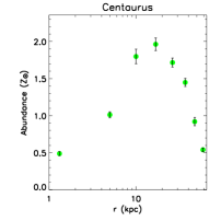
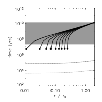
Figure 2: (Left) Best joint-fit of the gas density and temperature profile of the deprojected data of Centaurus (from s02 ) with a modified NFW gas profile. (Middle) Metal abundance profile with the characteristic central drop observed in spatially well resolved cool-core clusters. (Right) H-He (thick dotted line) and H-Fe (thin dotted line) equipartition time in the Centaurus cluster. The dots mark the radius $r_{\rm in}$ at which He is accumulated from the regions beyond with a sedimentation time represented by the solid line: $t_{\rm sed}=\int^{r_{\rm out}}_{r_{\rm in}}dr/v_{\rm sed}(r)$. The shaded region ranges between a $t_{\rm cool}=2\times 10^{7}$ yrs and the age of the Universe (details in ef06 ).

We have estimated the gravitational acceleration by fitting to the observed deprojected gas density and temperature profiles some functional forms that well reproduce the central steepening and are obtained under the assumption that the plasma is in the hydrostatic equilibrium with a NFW potential (left panel in Fig. 2). The observed gas density and temperature values do not allow metals to settle down in cluster cores over timescales shorter than few $10^{9}$ years. On the other hand, by assuming that in the same potential the gas that is now describing a cool core was initially isothermal, the sedimentation times are reduced by 1–2 order of magnitude within $0.2r_{200}$. The sedimentation of helium can then take place in cluster cores. Even modest enhancement in the helium abundance affects (i) the relative number of electron and ions $\frac{n_{\rm e}}{n_{\rm p}}=c_{M}=\sum M_{i}Z_{i}N_{i}=1+2M_{\rm He}N_{\rm He}+\sum_{i\neq{\rm H,He}}M_{i}Z_{i}N_{i}$, (ii) the atomic mean molecular weight $\mu=\left(\sum_{i}\frac{X_{i}(1+Z_{i})}{A_{i}}\right)^{-1}$ and all the X-ray quantities that depend on these values, such as the emissivity $\epsilon$, the gas mass density $\rho_{\rm g}\propto\mu(1+c_{M})$, the total gravitating mass, $M_{\rm tot}\propto\mu^{-1}$, the gas mass fraction, $f_{\rm gas}\propto\mu^{2}(1+c_{M})$. Moreover, we show in ef06 that if we model a super-solar abundance of helium with the solar value, we underestimate the metal (iron) abundance and overestimate the model normalization or emission measure. For example, with $M_{\rm He}=3$, the measured iron abundance and emission measure are $\sim 0.65$ and $1.5$ times the input values, respectively. Thus, an underestimated excess of the He abundance might explain the drops in metallicity observed in the inner regions of cool-core clusters (see, e.g., middle panel in Fig. 2). It is worth noticing that the diffusion of helium can be suppressed, however, by the action of confinement due to reasonable magnetic fields (see cl04 ), or limited to the very central region ($r<20$ kpc) by the turbulent motion of the plasma.

3 Iron in X-ray galaxy clusters

The iron abundance is nowadays routinely determined in nearby systems thanks mostly to the prominence of the K-shell iron line emission at rest-frame energies of 6.6-7.0 keV (Fe XXV and Fe XXVI). Furthermore, the few X-ray galaxy clusters known at $z>1$ have shown well detected Fe line, given sufficiently long ($>200$ ksec) Chandra and XMM-Newton exposures (r04 , h04 , to03 ). It is more difficult to assess the abundance of other prominent metals that should appear in an X-ray spectrum at energies (observer rest frame) between $\sim 0.5$ and $10$ keV, such as oxygen (O VIII) at (cluster rest frame) 0.65 keV, silicon (Si XIV) at 2.0 keV, sulfur (S XVI) at 2.6 keV, and nickel (Ni) at 7.8 keV. In e05 , we infer from observed and modeled SN rates the total and relative amount of metals that should be present in the ICM both locally and at high redshifts. Through our phenomenological approach, we adopt the models of SN rates as a function of redshift that reproduce well both the very recent observational determinations of SN rates at $z>0.3$ (d04 , c05 ) and the measurements of the star formation rate derived from UV-luminosity densities and IR data sets. We then compare the products of the enrichment process to the constraints obtained through X-ray observations of galaxy clusters up to $z\sim 1.2$.

Table 1: Adopted values for the average atomic weight ($W$), solar abundance by number with respect to H ($A$, from ag89 and a05 ; $R=A_{\rm A05}/A_{\rm AG89}$), total synthesized isotopic mass per SN event ($m_{Ia}$ from deflagration model W7 and $m_{CC}$ integrated over the mass range $10-50M_{\odot}$ with a Salpeter IMF; see n97 ) and corresponding abundance ratios by numbers with respect to Fe, $Y_{i}=m_{i}/(W_{i}A_{i})\times(W_{\rm Fe}A_{\rm Fe})/m_{\rm Fe}$.

metal	$W$	$A_{\rm AG89}$	$A_{\rm A05}$	$R$		$m_{Ia}$	$Y_{Ia}$	$m_{CC}$	$Y_{CC}$
						$M_{\odot}$		$M_{\odot}$
He	4.002	9.77e-2	8.51e-2	0.87		$-$	$-$	$-$	$-$
Fe	55.845	4.68e-5	2.82e-5	0.60		0.743	$-$	0.091	$-$
O	15.999	8.51e-4	4.57e-4	0.54		0.143	0.037	1.805	3.818
Si	28.086	3.55e-5	3.24e-5	0.91		0.153	0.538	0.122	3.526
S	32.065	1.62e-5	1.38e-5	0.85		0.086	0.585	0.041	2.284
Ni	58.693	1.78e-6	1.70e-6	0.95		0.141	4.758	0.006	1.647

The observed iron mass is obtained from dg04 and to03 (see also e04 ) as

$$M_{\rm Fe,obs}=4\pi A_{\rm Fe}W_{\rm Fe}\int_{0}^{R}Z_{\rm Fe}(r)\rho_{\rm H}(r)r^{2}dr,$$ (2)

where $Z_{\rm Fe}(r)$ is the radial iron abundance relative to the solar value $A_{\rm Fe}$, $W_{\rm Fe}$ is the iron atomic weight and $\rho_{\rm H}(r)$ is the hydrogen mass density. To recover the history of the metals accumulation in the ICM, we use the models of the cosmological rates (in unit of SN number per comoving volume and rest-frame year) of Type Ia, $r_{\rm Ia}$, and core-collapse supernovae, $r_{\rm CC}$, as presented in d04 and s04 . We estimate then the iron mass through the equation

$$M_{\rm Fe,SN}=M_{\rm Fe,Ia}+M_{\rm Fe,CC}=\sum_{dt,dV}\left(m_{\rm Fe,Ia}r_{\rm Ia}(dt)+m_{\rm Fe,CC}r_{\rm CC}(dt)\right)dtdV$$ (3)

where $m_{\rm Fe,Ia}$ and $m_{\rm Fe,CC}$ are quoted in Table 1, $dt$ is the cosmic time elapsed in a given redshift range, $dV$ is the cluster volume defined as the volume corresponding to the spherical region that encompasses the cosmic background density, $\rho_{\rm b}=3H_{0}^{2}/(8\pi G)\times\Omega_{\rm m}$ ($\approx 4\times 10^{10}M_{\odot}$ Mpc^-3 for the assumed cosmology), with a cumulative mass of $M_{\rm vir}\approx 6.8(kT/5{\rm keV})^{3/2}\times 10^{14}M_{\odot}$ (arn05 ). We obtain that these SN rates provide on average a total amount of iron that is marginally consistent with the value measured in galaxy clusters in the redshift range $0-1$, and a relative evolution with redshift that is in agreement with the observational constraints up to $z\approx 1.2$. We predict metals-to-iron ratios well in agreement with the X-ray measurements obtained in nearby clusters implying that (1) about half of the iron mass and $>$ 75 per cent of the nickel mass observed locally are produced by SN Ia ejecta, (2) the SN Ia contribution to the metal budget decreases steeply with redshift and by $z\approx 1$ is already less than half of the local amount and (3) a transition in the abundance ratios relative to the iron is present at $z$ between $\sim 0.5$ and $1.4$, with SN CC products becoming dominant at higher redshifts.

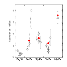
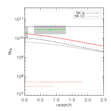
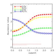
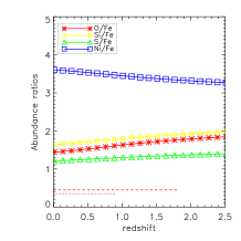
Figure 3: (From left to right, from up to bottom): (A) SN Ia rates and number ratio of SNe CC to Ia as a function of $z$ for the delay time distribution functions $\phi(t_{d})$ considered in d04 (dashed lines) and m06 (the solid line is the sum of the contribution from “tardy”/squares and “prompt”/dots population). (B) Predictions (big dots; using $\phi(t_{d})$ from m06 ) of the local metal ratios compared with the X-ray measurements in ta04 and b05 . (C) Accumulation history of the iron mass, $M_{\rm Fe}$, as obtained from eq. (3) with rates from m06 . The solid line shows the sum of SN Ia (dashed line) and SN CC (dotted line) contribution. The accumulation history is here compared to the total iron mass measured in samples of local (dg04 ) and high$-z$ (to03 ) clusters for a typical object at 5 keV. (D) Observed (ba06 ) and predicted (as in panel A and normalized to the observed value at $z\approx 0.4$) iron abundance as function of redshift. (E-F) The last two plots show the metal abundance ratios as function of redshift as predicted from a $\phi(t_{d})$ described by a “narrow” Gaussian with $\tau=4$ Gyr and $\sigma_{t_{d}}=0.2\tau$ as in d04 (E; see the corresponding rates in panel A) and from a bi-modal SN Ia distribution as in m06 (F). Horizontal lines indicate the redshift region where the SN rates are actually measured. These calculations refer to the solar abundance values in ag89 for a direct comparison with the data. By adopting the compilation in a05 , the trends are confirmed with the most relevant change being the predicted Ni/Fe$\approx 2$ at $z=0$.

Recently, Mannucci et al. (2006; see also sr05 ) argue that the data on (i) the evolution of SN Ia rate with redshift, (ii) the enhancement of the SN Ia rate in radio-loud early type galaxies and (iii) the dependence of the SN Ia rate on the colours of the parent galaxies suggest the existence of two populations of progenitors for SN Ia, one half (dubbed “prompt”) that is expected to occur soon after the stellar birth on time scale of $10^{8}$ years and is able to pollute significantly their environment with iron even at high redshift, the other half (“tardy”) that has a delay time function consistent with an exponential function with a decay time of $\sim 3$ Gyrs. Due to the larger production of SN Ia at higher redshift (see panel A in Fig. 3), the rates suggested by Mannucci et al. predict a more flat distribution of the Fe abundance as function of $z$ than the rates tabulated in d04 , but still show a negative evolution partially consistent with the measurements up to $z\approx 1.2$ (panel D in Fig. 3). Furthermore, these rates provide a better agreement than the ones in d04 both with local abundance ratios (panel B in Fig. 3) and with the overall production of Fe (panel C), that at $z=0$ has been released from SNe Ia by more than 60 per cent. A potential discriminant is the behaviour of the abundance ratios relative to Fe in the ICM as a function of redshift, providing the rates in m06 values of O/Fe and Ni/Fe that are a factor of 2 different from the predictions of the single-population delay time distribution function (see panels E and F).

References

- (1) Anders E., Grevesse N.: Geochimica et Cosmochimica Acta, 53, 197 (1989)
- (2) Arnaud M., Pointecouteau E., Pratt G.W.: A&A, 441, 893 (2005)
- (3) Asplund M., Grevesse N., Sauval A.J.: “Cosmic abundances as records of stellar evolution and nucleosynthesis”, eds. Bash F.N. and Barnes T.G., ASP Conf. Series, 336, 25 (2005)
- (4) Balestra I. et al.: A&A, in press (2006; astro-ph/0609664)
- (5) Baumgartner W.H. et al.: ApJ, 620, 680 (2005)
- (6) Cappellaro E. et al.: A&A, 430, 83 (2005)
- (7) Chuzhoy L., Loeb A.: MNRAS, 349, L13 (2004)
- (8) Dahlen T. et al.: ApJ, 613, 189 (2004)
- (9) De Grandi S., Ettori S., Longhetti M., Molendi S.: A&A, 419, 7 (2004)
- (10) Grevesse N., Sauval A.J.: Space Science Rev., 85, 161 (1998)
- (11) Ettori S.: MNRAS, 344, L13 (2003)
- (12) Ettori S., Tozzi P., Borgani S., Rosati P.: A&A, 417, 13 (2004)
- (13) Ettori S.: MNRAS, 362, 110 (2005)
- (14) Ettori S., Fabian A.C.: MNRAS, 369, L42 (2006)
- (15) Hashimoto Y. et al.: A&A, 417, 819 (2004)
- (16) Mannucci F., Della Valle M., Panagia N.: MNRAS, 370, 773 (2006)
- (17) Nomoto K. et al.: Nucl. Phys. A, 621, 467 (1997)
- (18) Rosati P. et al.: AJ, 127, 230 (2004)
- (19) Sanders J.S., Fabian A.C.: MNRAS, 331, 273 (2002)
- (20) Scannapieco E., Bildsten L.: ApJ, 629L, 85 (2005)
- (21) Spergel D.N. et al.: ApJ, submitted (2006; astro-ph/0603449)
- (22) Spitzer L.: Physics of Fully Ionized Gases (Interscience Publishers, New York 1956)
- (23) Strolger L.G. et al.: ApJ, 613, 200 (2004)
- (24) Tamura T. et al.: A&A, 420, 135 (2004)
- (25) Tozzi P. et al.: ApJ, 593, 705 (2003)
Index
- A3526 Figure 2